Yield Gap Analysis of Alfalfa Grown under Rainfed Condition in Kansas

Abstract

The yield and production of alfalfa (Medicago sativa L.) have not been significantly improved in Kansas for the last 30 years even though farmers are using improved varieties. We have noted a significant yield difference between average alfalfa yield reported by farmers and researchers. The magnitude of yield gap in Kansas and its underlying factors are still unknown. Thus, understanding of potential yield is essential to meet the future forage demand with the limited production resources. The main objective of this study was, therefore, to quantify the current yield gap and identify the main yield-limiting factor for rainfed alfalfa grown in Kansas. To achieve this objective, we selected 24 counties in Kansas based on the rainfed production area and total production, and used county-level yield, daily temperature, and rainfall data from the past 30 yrs (1988–2017) of those selected counties. We applied four statistical approaches: (i) probability distribution function to delineate county-level alfalfa growing season, (ii) stochastic frontier yield function to estimate optimum growing season rainfall (GSR) and attainable yield, (iii) linear boundary function to estimate minimum water loss, water use efficiency, and water-limited potential yield, and (iv) conditional inference tree to identify the major yield contributing weather variables. The probability distribution function delineated the alfalfa growing season starting from mid-March to mid-November in Kansas. The frontier model estimated the attainable yield of 9.2 Mg ha⁻¹ at an optimum GSR of 664 mm, generating a current yield gap of 18%. The linear boundary function estimated the water-limited potential yield of 15.5 Mg ha⁻¹ at an existing GSR of 624 mm, generating a yield gap of 50%. The conditional inference tree revealed that 24% of the variation in rainfed alfalfa yield in Kansas was explained by weather variables, mainly due to GSR followed minimum temperature. However, we found only 7% GSR deficit in the study area, indicating that GSR is not the only cause for such a wide yield gap. Thus, further investigation of other yield-limiting management factors is essential to minimize the current yield gap. The statistical models used in this study might be particularly useful when yield estimation using remote sensing and crop simulation models are not applicable in terms of time, resources, facilities, and investments.

1. Introduction

Alfalfa (Medicago sativa L.), also called Lucerne, is a perennial leguminous plant cultivated as forage for livestock animals. It is grown extensively worldwide because of its multiple benefits, such as high forage yield, high nutritive value, and biological nitrogen fixation [1,2]. It is the third largest field crop in the United States (US) and the fourth in Kansas, USA, in terms of economic value. Kansas ranked as the 7th largest alfalfa-producing state in the USA in 2021, where annual alfalfa hay production exceeded 2.5 million tons from about 0.7 million hectares [3].

Alfalfa crop yields have been widely investigated, particularly to determine if crop yields are influenced by the interaction of genotype, environment and management factors [4]. Among several yield determining factors, water is the main yield driving abiotic factor for alfalfa because alfalfa requires a relatively higher amount of water compared to other field crops [5,6,7,8]. Baral et al. [9] revealed that growing season rainfall (GSR) is one of the main yield-limiting factors for rainfed alfalfa production in the US. In Kansas, more than 78% of alfalfa is grown under rainfed conditions [3]. The amount and distribution of rainfall during growing season plays a key role for alfalfa growth, regrowth, and total biomass yield. The irrigation requirement varies from 356 mm in east Kansas to 686 mm in west Kansas, as western Kansas receives a lot less rainfall than eastern Kansas [10,11,12]. Additionally, western Kansas has been experiencing moderate to exceptional drought for decades during the alfalfa growing season (GS) (April-October) [12], which is the major challenge for non-irrigated alfalfa because drought can reduce the yield by up to 70% [8].

On the other hand, Kansas farmers have been using improved alfalfa seeds, such as lower-lignin and Roundup Ready traits, even though the yield has almost stagnated at 8.4 Mg ha⁻¹ and production has declined by approximately 25% in the last 30 years [3]. However, various field-based research carried out in Kansas in the past shows yields of >15 Mg ha⁻¹ in Kansas [13,14,15]. The reason behind alfalfa production decline could be due to the severe to extreme droughts observed periodically in many parts of Kansas [16] and the expansion of soybean and corn production areas during the last 20 years [3]. However, to the best of our knowledge, the main reason behind yield difference between farmers’ reported yield and research reported yield for Kansas has not been documented. It is thus important to estimate the yield potential, understand the current yield gap and its causal factors in alfalfa in Kansas.

In recent years, remote sensing models [17,18,19,20] and crop simulation models [21,22,23,24] have been commonly used as reliable models for crop yield and yield gap estimation. However, those models require time and field-specific daily weather data (such as CO₂, solar radiation, temperature, rainfall, relative humidity, wind speed, evapotranspiration), management practices (such as planting date, plant density, harvesting time), soil properties, initial soil water content, and plant growth measurement, and investment [21,24].

Thus, the main objective of this study is to estimate the water-limited potential yield and yield gap of alfalfa grown under rainfed conditions in Kansas using historical yield and weather data. More specifically, this study (i) delineates county-specific alfalfa growing season, (ii) estimates county-level attainable and potential yield and compares with current yield, and (iii) identifies the most yield-limiting weather variable in alfalfa production in Kansas.

2. Materials and Methods

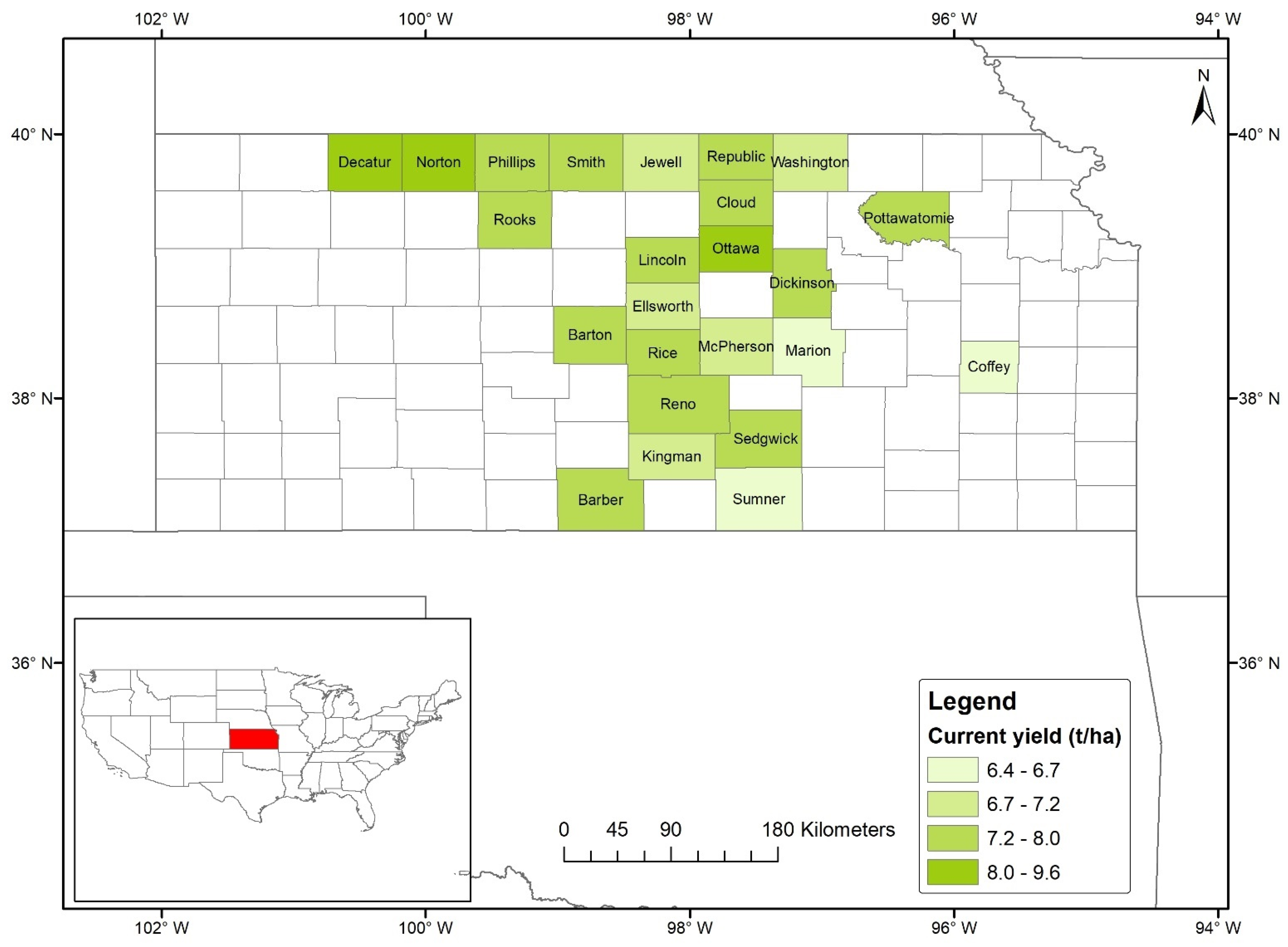
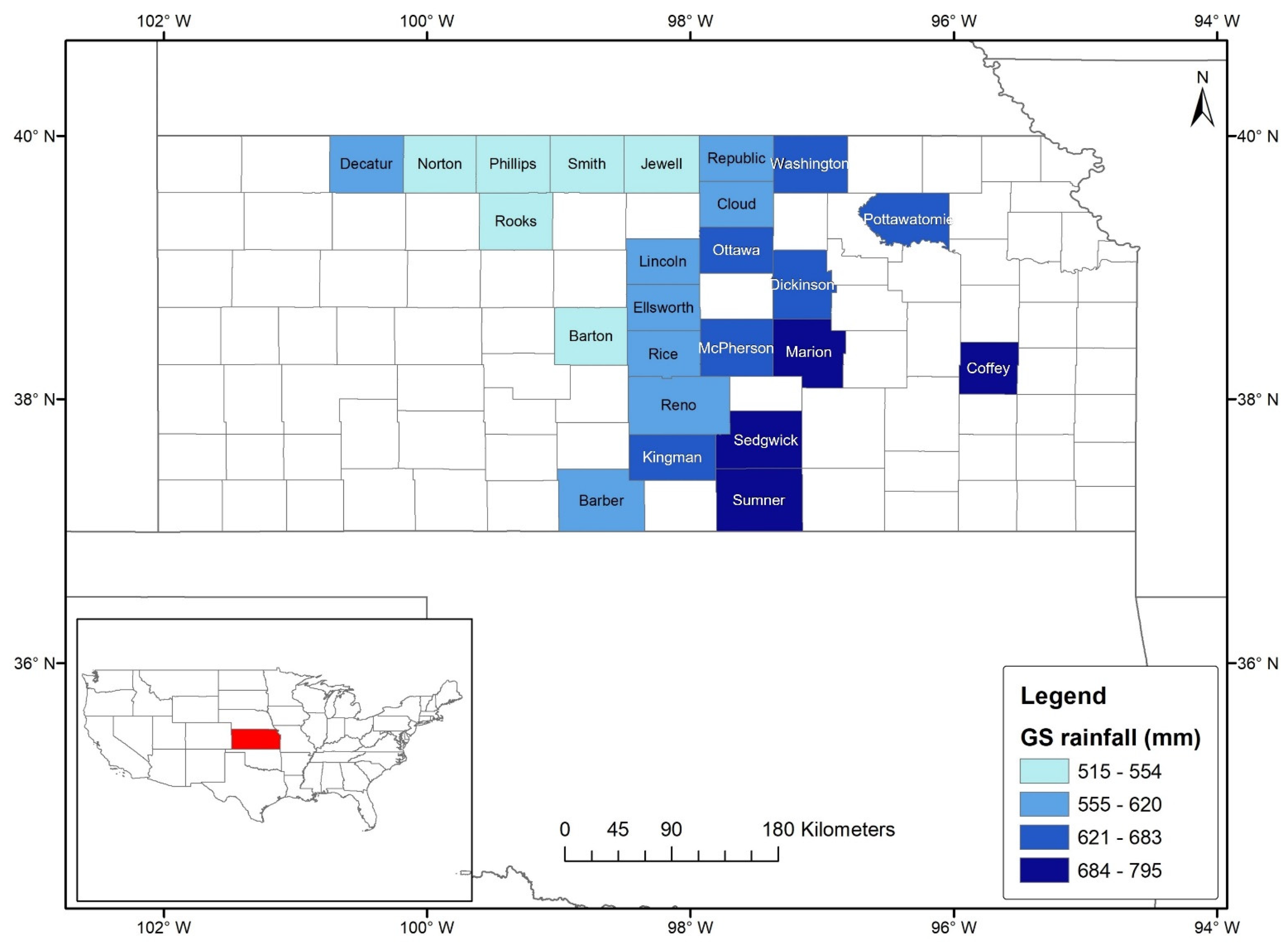
2.1. Study Site

The study area was selected based on the rainfed alfalfa production area and total production. The rainfed counties were selected based on two criteria: (i) less than 5% irrigated area and (ii) more than 1% of the total alfalfa production in Kansas. Of the 105 counties in Kansas, only 24 counties met those two criteria [3] (Figure 1).

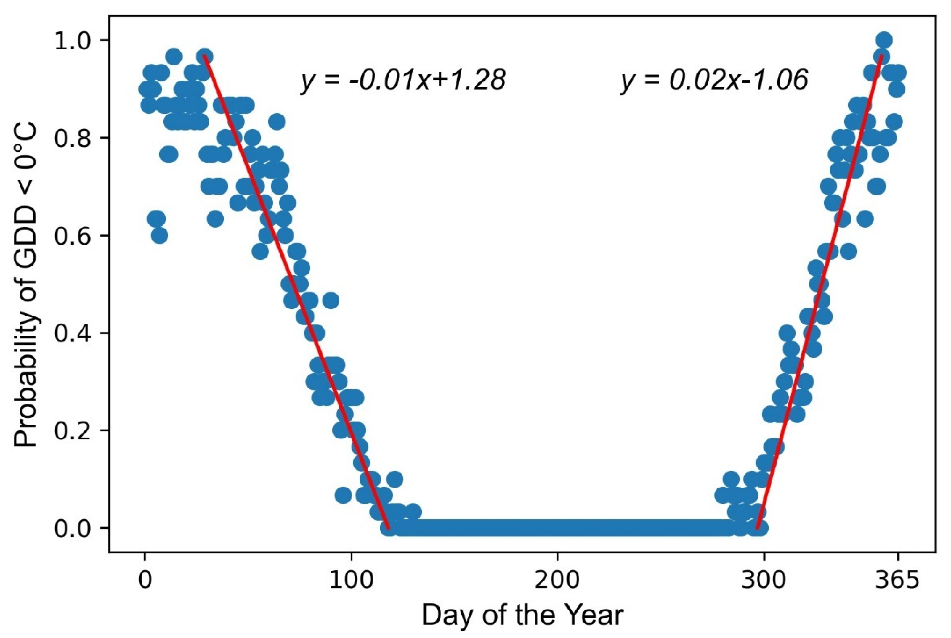
2.2. Defining Growing Season

The daily maximum and minimum temperature and rainfall data of all selected counties were collected for the last 30-yr period (1988–2017) from PRISM Climate Group [24]. The growing degree day (GDD) of each day of the year for the study period was calculated by using the following formula.

$$\mathrm{GDD}=\frac{\mathrm{Tmax}+\mathrm{Tmin}}{2}-\mathrm{Tbase}$$

(1)

where GDD represents growing degree day of each day of a year, Tmax represents maximum temperature and Tmin represents minimum temperature of a day, and Tbase represents base temperature below which growth rate equals zero. The widely used base temperature for alfalfa is 5 °C [25,26,27]. Then, we followed the same approach used by Baral et al. [9], Purcell et al. [28] and Torres et al. [29], who used the probability distribution function to delineate the growing season. The alfalfa GS was estimated as the duration (cumulative GDD) between the last day in the spring and the first day in the fall when there is zero probability of occurrence of GDD less than 0 °C (Figure 2). The cumulative GDD within the growing season is termed as growing season thermal units, and the cumulative rainfall as GSR for the particular county.

2.3. Yield Estimation

We estimated three types of yields: (i) current yield (Y_c) (ii) attainable yield (Y_a) and (iii) water-limited potential yield (Y_w) of alfalfa using government-reported alfalfa hay yield, daily temperature and rainfall data of the selected 24 counties in Kansas from the past 30 years (1998–2017). The annual county-level yield data were collected from the USDA-NASS database [3].

There is insignificant variation on forage dry matter yield over the last 30 years. Thus, we defined Y_c as the mean yield of alfalfa hay that was achieved by a county within the last 30 years from farmers’ fields using Equation (2):

$$Y_{c }={{\displaystyle \sum }}_{i=1}^n\frac{Y}{N}$$

(2)

where $Y_c$ is the county-level mean yield, Y is the last 30 year’s annual alfalfa hay yield of a county and N is the number of years.

Y_a is defined as the maximum yield of alfalfa hay that was ever achieved by a county within the last 30 years in the existing production environment. We used the Cobb–Douglas stochastic frontier yield function used by Baral et al. [9], Neumann et al. [30] and Patrignani et al. [31] to estimate Y_a (Figure 3A). In this method, the growing season rainfall was divided into small bins and the maximum yield value from each bin was selected. Those selected values were then connected with frontier regression line using Equation (3):

$$ln{Y}_a={\beta }_0+{\beta }_{1}ln{X}_i+{\beta }_2(ln{X}_i^2),X_i>0$$

(3)

where $Y_a$ represents the attainable yield (the maximum yield achieved by county $i$ within the last 30 years within each rainfall bin), $X_i$ represents the corresponding growing season rainfall of county $i$, ${\beta }_0$ was the intercept when yield is zero, and ${\beta }_1$ and ${\beta }_2$ were the coefficients of first and second order of logarithm value of the growing season rainfall, respectively. Under an efficient level of production, the maximum yield value found on the frontier line is referred as the Y_a and the corresponding rainfall as optimum rainfall to achieve maximum yield for a county (Figure 3A). The optimum GSR at which the yield is maximum was determined by equating the partial derivative of the frontier yield with respect to GSR to zero, and then solving Equation (3) for this particular rainfall amount.

Water-limited potential yield (Y_w) is defined as the maximum possible yield of a county that can be achieved at a given amount of GSR without limiting the yield by nutritional, management, and other production factors, such as land, labor, capital, insect pest, and disease. We used the linear boundary function adopted by Baral et al. [9] and French and Schultz [32] to estimate Y_w (Figure 3B). We followed the same method used to estimate Y_a, but we also incorporated yield data obtained from research experiments assuming that water and nutrient non-limiting factors. Equation (4) is the regression equation we used to estimate county-level Y_w:

$$ln{Y}_w={\beta }_0+{\beta }_{1}lnX, x>0$$

(4)

where $Y_w$ represents theoretical water-limited potential yield that can be obtained from the use of available growing season rainfall data determined by the frontier line in Equation (2), ${\beta }_0$ is the x-intercept of the GSR (which defines minimum non-productive water losses from the soil) and ${\beta }_1$ is the slope of the yield-rainfall relationship (which defines water use efficiency (WUE)), and $X$ was the amount of water used by the plant during the entire growing season to obtain maximum potential yield. The estimation was based on the assumption that: (i) nutritional and other production factors, such as variety, insect, pest and diseases, are effectively managed, (ii) minimum loss of soil water due to surface runoff or leaching during growing season, (iii) low soil water storage during winter, and (iv) insignificant variation in soil properties or water holding capacity of the soil in all alfalfa growing counties. Field experiment data were also used for the best fit of linear line (Figure 3B). The experiment data was taken from Manhattan, Garden City, and Colby Kansas [13,14,15] assuming that those yields were not limited by nutritional and management practices.

The yield gap (Y_g) was calculated by deducting the county-level mean yield with estimated Y_a or Y_w.

$$YGa=Y_a-Y_c$$

(5)

$$YGw=Y_w-Y_c$$

(6)

where, YGa represents current yield gap compared to attainable yield, and YGw represents current yield gap compared to water-limited potential yield.

2.4. Yield Determining Weather Variables

We used conditional inference tree (CIT), a correlation-based, unbiased, recursive partitioning method, to identify the most yield-determining weather variable in a conditional tree framework [33,34]. The “ctree” function and “partykit” package in R programming was used to perform this analysis. The alfalfa dry matter yield values of 24 counties from 1988 to 2017 were used as the response variable, and alfalfa GSR, Tmin, Tmax, and cumulative thermal unit of the same period as the explanatory variables.

3. Results

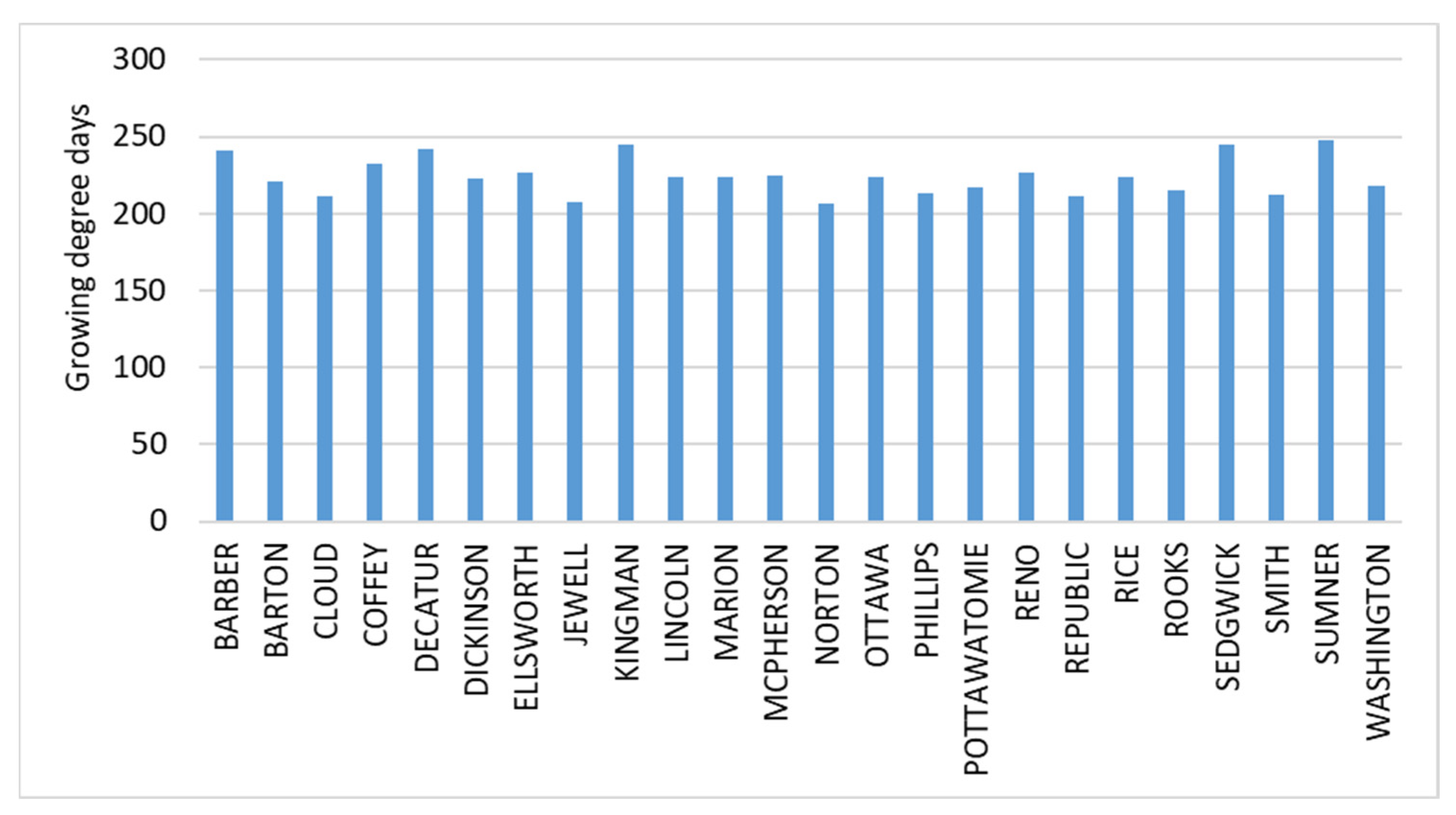
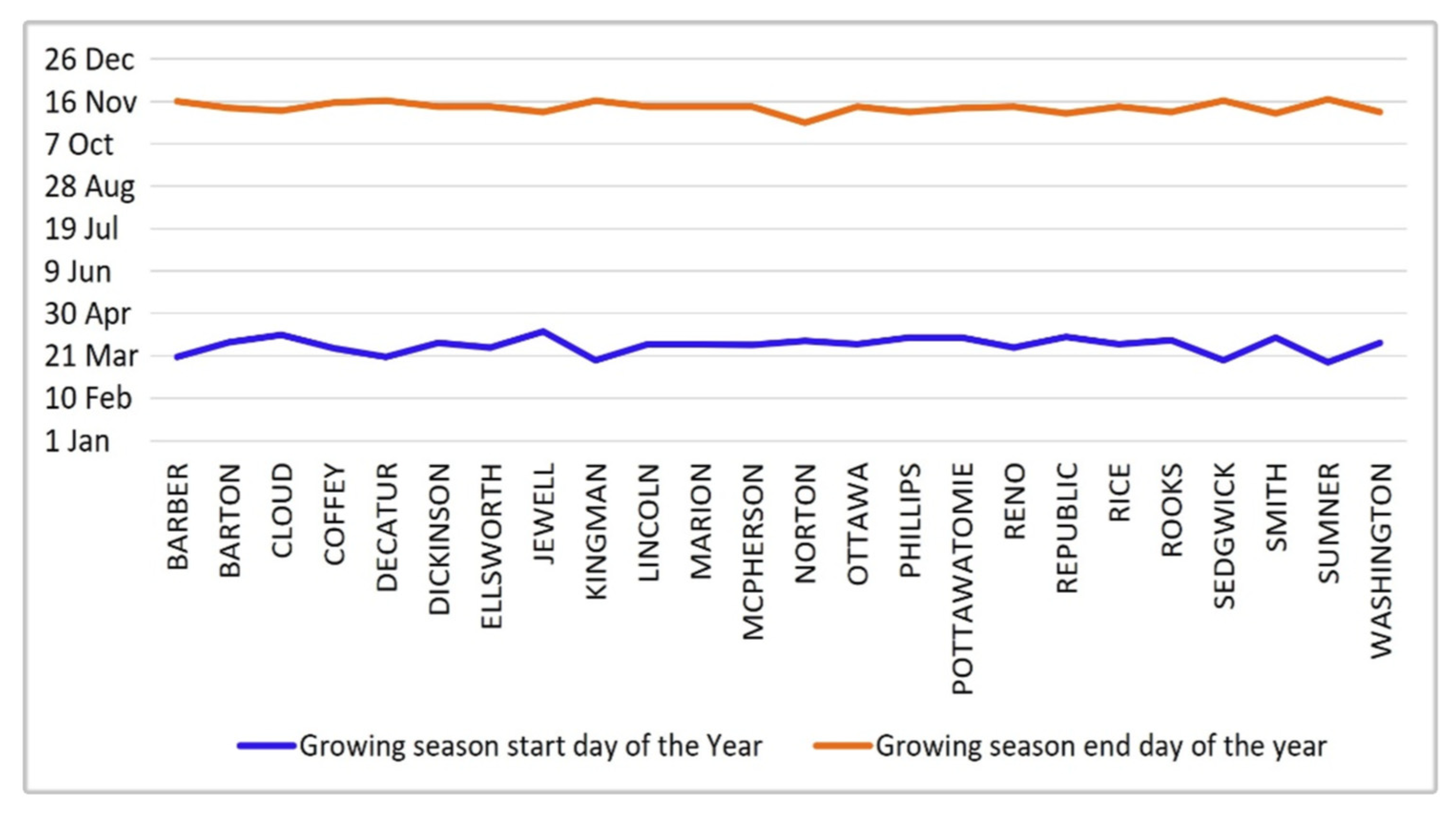
3.1. Growing Season Delineation

The length of the alfalfa GS determines the number of cuttings per season and the yield of alfalfa. The length of the alfalfa GS for the selected rainfed counties in Kansas ranged from 206 days in Norton County to 248 days in Sumner County, with a mean of 224 ± 12 days in a year (Figure 4). Barber, Decatur, Kingman, Sedgwick and Sumner Counties have longer growing seasons (>240 days) than other selected counties.

Our study revealed that the alfalfa GS for Kansas starts from mid-March (South Kansas) to mid-April (North Kansas) and ends within around mid-November (Figure 5).

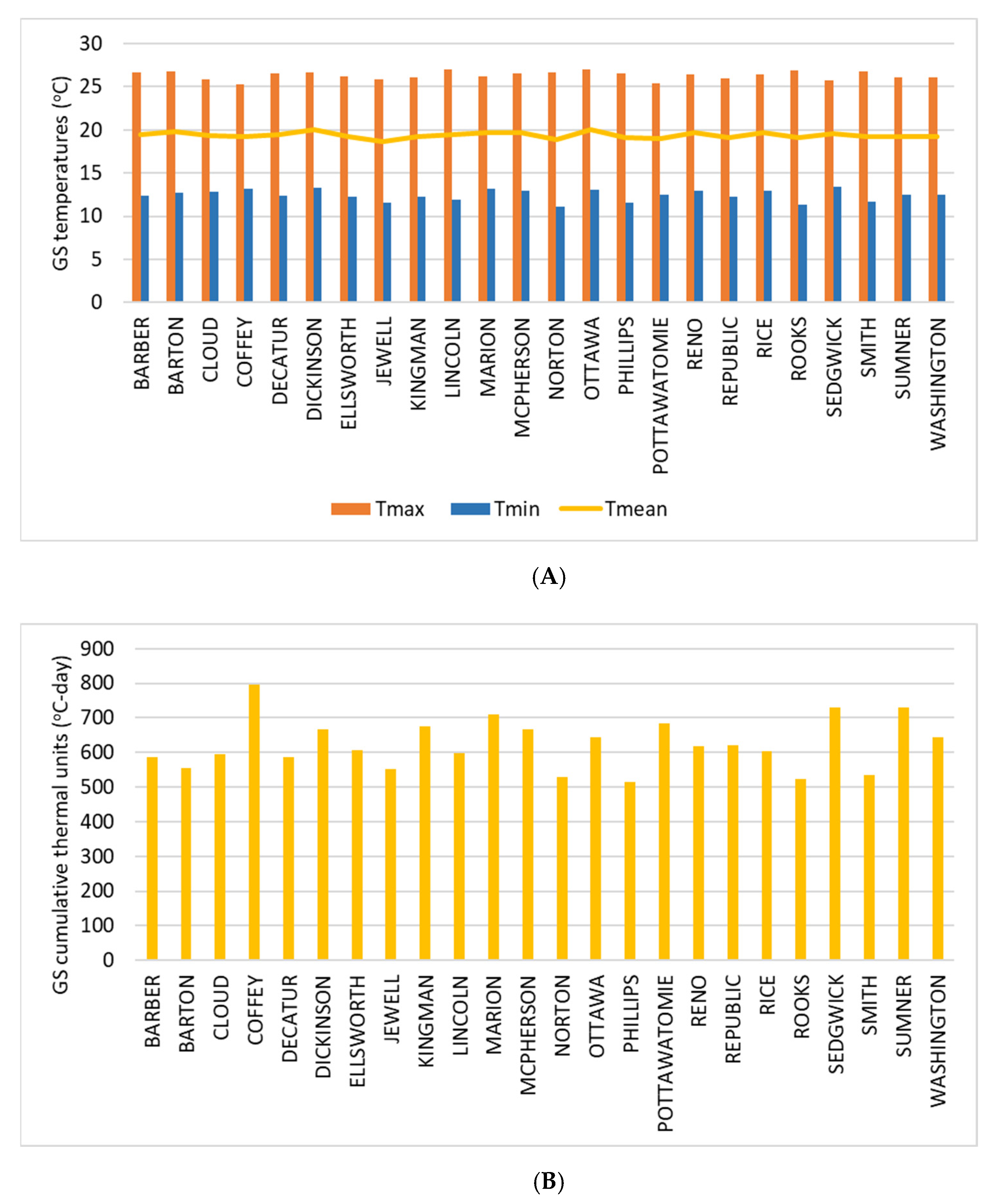
3.2. Growing Season Rainfall, Temperature and Thermal Units

Over the 30-yr period (1988–2017), the mean annual rainfall of the selected counties ranged from 514 mm in Phillips County to 795 mm in Coffey County, with a mean value of 624 ± 72 mm (Figure 6). Growing season rainfall of Coffey, Marion, Sedgwick, and Sumner County was found to be higher (>700 mm) than the other selected counties.

The mean growing season maximum temperature was found to be 26.3 ± 0.5 °C and the minimum temperature was 12.4 ± 0.6 °C (Figure 7A). Similarly, the cumulative mean growing season thermal units were estimated to be 3164 ± 200 °C-day for the rainfed counties. Barber, Kingman, and Rooks Counties had the highest growing season cumulative thermal units (above 3400 °C-day) among the selected counties (Figure 7B).

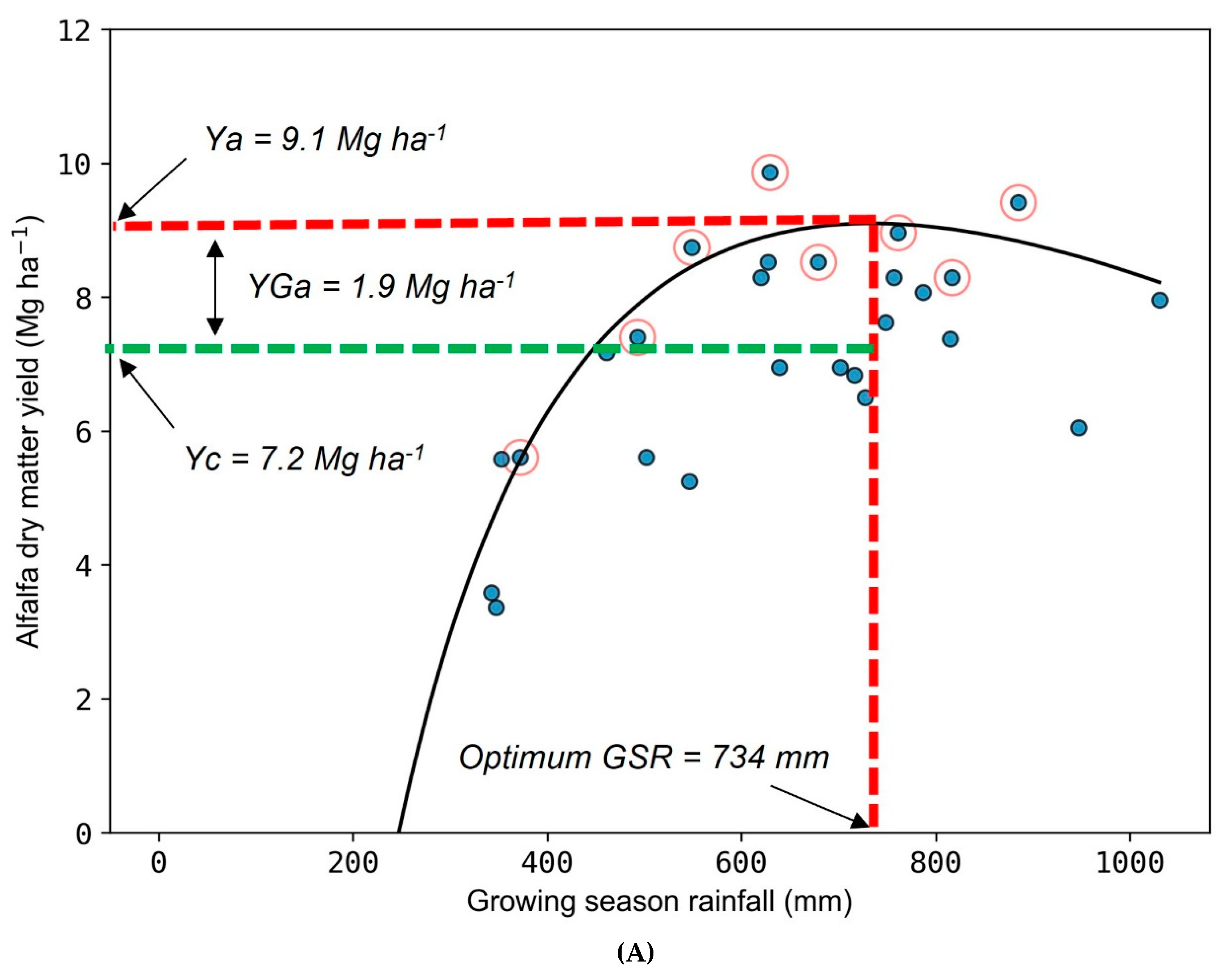
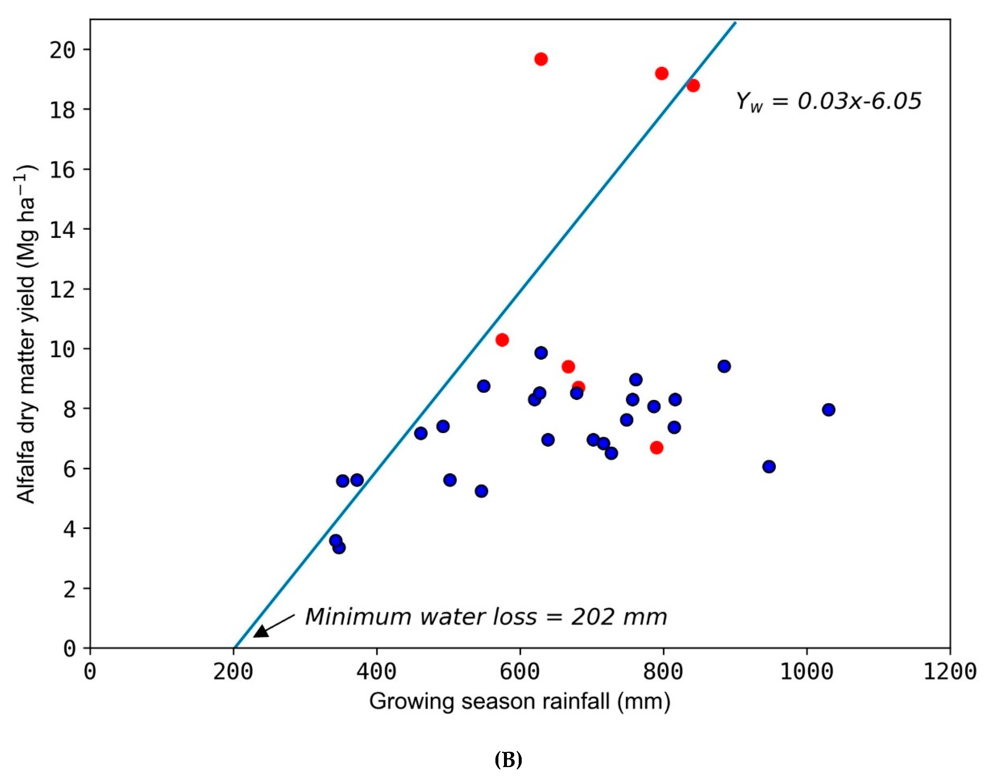
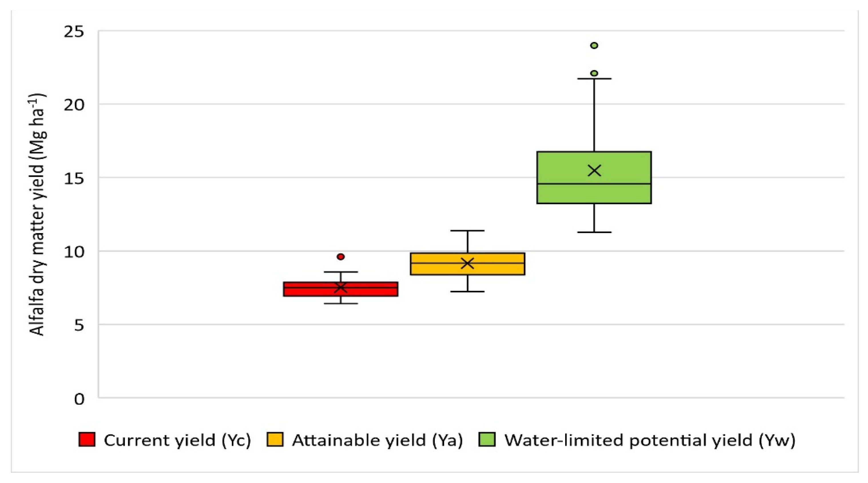
3.3. Alfalfa Yields, Yield Gaps and WUE

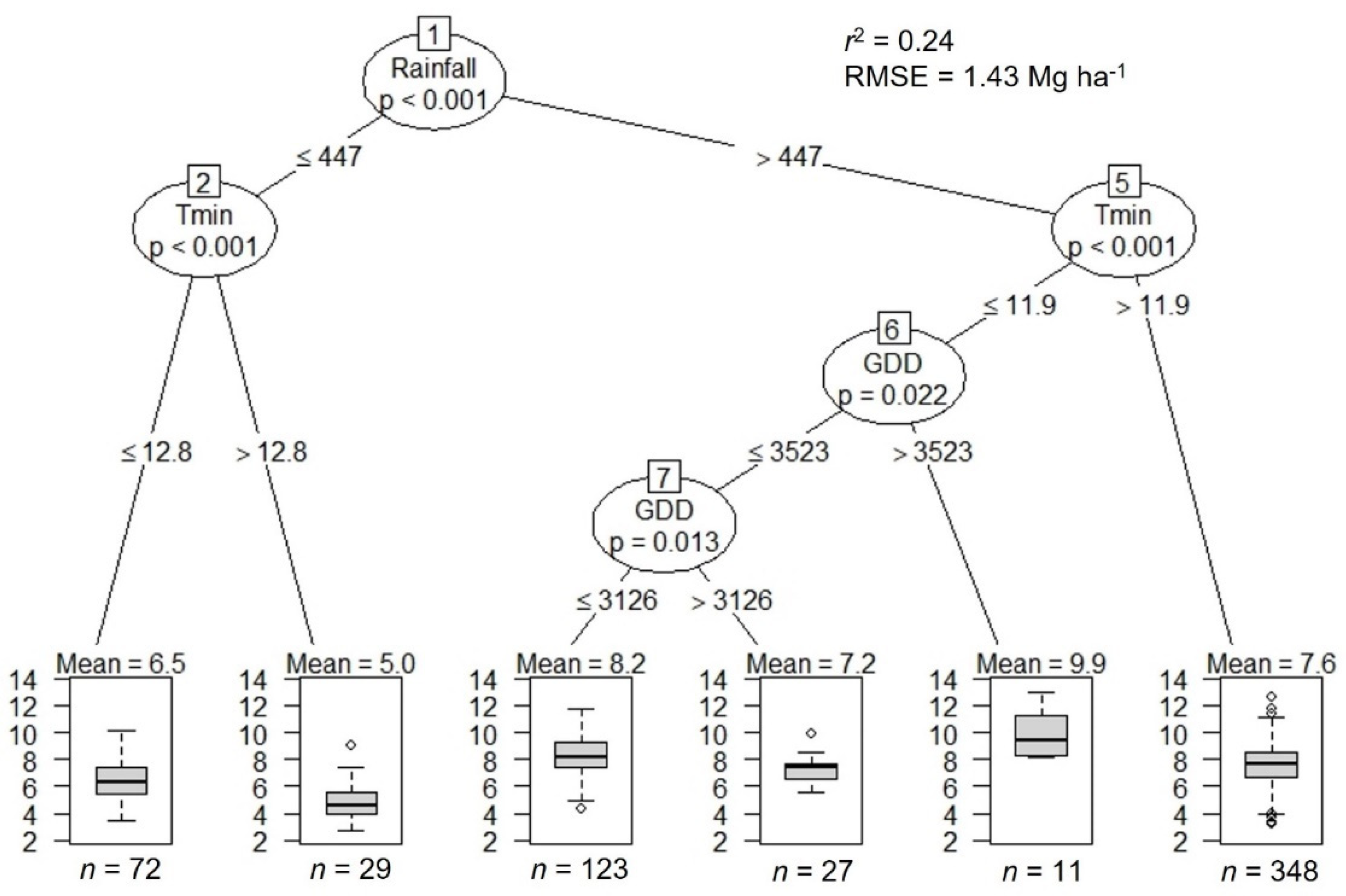
The mean alfalfa yield (Y_c) ranged from 6.4 Mg ha⁻¹ in Marion County to 9.6 Mg ha⁻¹ in Decatur County, with a mean value of 7.5 Mg ha⁻¹ [3] over the period of 30-yrs (Figure 8).

Our frontier model predicted an alfalfa Y_a of 9.2 Mg ha⁻¹ at an optimum GSR of 664 mm, creating a yield gap of 18% (Figure 8, Supplementary Table S1). The linear boundary function estimated a mean Y_w of 15.5 Mg ha⁻¹ at the mean GSR of 624 mm, creating a yield gap of 50% (Figure 8). Cloud County had the highest Y_w (24 Mg ha⁻¹) with a 69.3% yield gap, and Smith County had the lowest Y_w (11.3 Mg ha⁻¹) with a 31.3% yield gap. Similarly, the boundary function analyses estimated the potential alfalfa WUE, indicated as the slope of the boundary function between GSR and alfalfa yield, at 36 kg ha⁻¹ mm⁻¹, with mean evaporation of 188 mm (or 30% of mean GSR) (Supplementary Table S2).

3.4. CIT Analysis

The CIT analysis described a 24% yield variation across the 24 counties in the 30-year period with a RMSE of 1.43 Mg ha⁻¹, suggesting that GSR and Tmin were the most significant yield determining factors in Kansas (Figure 9). The analysis revealed that the highest DMY (8.2 Mg ha⁻¹) was obtained in areas where the rainfall was above 447 and Tmin below 11.9 °C during alfalfa GS, whereas the low yield (~6 Mg ha⁻¹) was found in the areas of GSR below 447 mm.

4. Discussion

Potential yield and yield gap have been estimated for several field crops at different scales such as global, regional or farm scale using various models including crop simulation model and remote sensing models. Although the crop simulation model is considered to be the most reliable method of predicting potential yields [21], it requires time, resources, facilities, and investments to establish research experiments and collect daily quantitative and qualitative data, such as soil moisture, leaf area index, evapotranspiration, atmospheric CO₂, solar radiation, and temperature and rainfall data. Furthermore, the crop simulation model may not be applicable for alfalfa because of its perennial nature, multiple harvests during the GS, and inconsistent harvesting intervals and yields per harvest within a season. Thus, we used a probability distribution function to estimate alfalfa GS and GSR, the frontier yield function model to estimate optimum GSR and Y_a, and a boundary linear model to estimate WUE and Y_w. These models are commonly used models to estimate potential yield [9,31] where remote sensing and crop simulation models are not applicable. Our estimated GS durations were aligned with the alfalfa GS recommended by Kansas State University forage agronomists (Shroyer et al., 1987). Likewise, the county level Y_w range (15.5 ± 3.1 Mg ha⁻¹) was found within the yield range (13.3–22.4 Mg ha⁻¹) estimated by Fink [35], and the yield obtained from the research experiments carried out at Riley, Finney, and Thomas Counties, Kansas [13,14,15].

The WUE, explained by the linear regression line in Figure 3B, is slightly greater than the WUE estimated by Fink [35] who estimated 33 kg ha⁻¹ mm⁻¹. The slight variation is probably due to the inclusion of a wider area and variation in weather conditions, as our CIT analysis explained that 24% of the yield variation in the study area was due to weather variables. Our study area was mostly confined to central Kansas, where the mean GSR is 624 ± 72 mm. Our model predicted an approximately 30% minimum water loss from the soil, while the remaining 70% is mostly used by plants, which was within the range found in previous studies [36,37,38].

The CIT analysis illustrated that GSR and minimum temperature are the two most significant yield determining weather variables. However, the study areas had only 7% rainfall deficit during alfalfa GS (Supplementary Table S2), suggesting that GSR is only limiting 7% of the total production environment in Kansas. In other words, management practices, such as variety selection, planting time adjustment, soil fertility, weed, irrigation, fertilizer and pest management, have a positive correlation with yield and, therefore, the existing yield gap could be due to improper management practices or poor soil health. Furthermore, the highest yield gap, found in Cloud County, had a sufficient amount of GSR even though the yield gap is 69% (Supplementary Tables S1 and S2). Thus, the current yield gap found in this study is not only due to the water-limited condition, and rather it could be due to management factors or soil limitations such as low water holding capacity, poor drainage, impervious soil layers, sloping land with excessive runoff. Further research is essential to explore the other yield-limiting factors in Kansas.

5. Conclusions

Our study found that 24 counties in the State of Kansas produce alfalfa under rainfed conditions. The optimum GSR required to produce the maximum yield for alfalfa was estimated to be 664 mm. The mean yield gap in the rainfed alfalfa growing counties in Kansas was estimated at 18% of the attainable yield (Y_a) and 50% of the water-limited potential yield (Y_w). The CIT analysis identified that the alfalfa GSR and Tmin are the two most significant yield-determining variables for rainfed alfalfa production in Kansas.

This study provides the evidence of the current yield gap in the rainfed alfalfa producing counties in Kansas, and also of its underlying factors, which are particularly relevant for alfalfa growers and service providers, including extension agents, crop consultants for better planning, tactical and strategic management, and yield forecasters. At the same time, it could be an important document that could help local governments and policymakers to develop strategies that can address the current yield gap in Kansas. This study also provides a reliable method to estimate the growing season of a particular crop for a specific location, and to estimate the yield gap when remote sensing and crop simulation models are not applicable. Thus, the finding of this study is relevant from farm management, policymaking, and research perspectives.

References

1. Putnam, D.H.; Summers, C.G.; Orloff, S.B. Alfalfa production systems in California. In Irrigated Alfalfa Management for Mediterranean and Desert Zones; University of California, Division of Agriculture and Natural Resource Publication 8287: Davis, CA, USA, 2007; pp. 1–19. Available online: https://alfalfa.ucdavis.edu/irrigatedalfalfa/pdfs/ucalfalfa8287prodsystems_free.pdf (accessed on 9 October 2021).
2. Adhikari, L.; Missaoui, A.M. Nodulation response to molybdenum supplementation in alfalfa and its correlation with root and shoot growth in low pH soil. J. Plant Nutr. 2017, 40, 2290–2302. [Google Scholar] [CrossRef]
3. USDA-NASS. Data and Statistics. United States Department of Agriculture, National Agricultural Statistics Service. Available online: https://www.nass.usda.gov/Data_and_Statistics/index.php (accessed on 10 January 2022).
4. Adhikari, L.; Baral, R.; Paudel, D.R.; Min, D.; Makaju, S.O.; Poudel, H.; Acharya, J.P.; Missaoui, A. Cold stress in plants: Strategies to improve cold tolerance in forage species. Plant Stress 2022, 4, 100081. [Google Scholar] [CrossRef]
5. Jia, Y.; Li, F.M.; Zhang, Z.H.; Wang, X.L.; Guo, R.; Siddique, K.H. Productivity and water use of alfalfa and subsequent crops in the semiarid Loess Plateau with different stand ages of alfalfa and crop sequences. Field Crops Res. 2009, 114, 58–65. [Google Scholar] [CrossRef]
6. Takele, E.; Kallenbach, R. Analysis of the Impact of Alfalfa Forage Production under Summer Water-Limiting Circumstances on Productivity, Agricultural and Growers Returns and Plant Stand. J. Agron. Crop. Sci. 2001, 187, 41–46. [Google Scholar] [CrossRef]
7. Schneekloth, J.; Andales, A. Seasonal Water Needs and Opportunities for Limited Irrigation for Colorado Crops; Colorado State University Extension: Fort Collins, CO, USA, 2017; Available online: https://extension.colostate.edu/topic-areas/agriculture/seasonal-water-needs-and-opportunities-for-limited-irrigation-for-colorado-crops-4-718/ (accessed on 10 October 2021).
8. Shewmaker, G.E.; Allen, R.G.; Neibling, W.H. Alfalfa Irrigation and Drought; University of Idaho, College of Agricultural and Life Sciences: Moscow, ID, USA, 2011. Available online: https://efotg.sc.egov.usda.gov/references/public/UT/AlfalfaIrrigationFacts2013Final.pdf (accessed on 15 October 2021).
9. Baral, R.; Lollato, R.P.; Bhandari, K.; Min, D. Yield Gap Analysis of Rainfed Alfalfa in the United States. Front. Plant Sci. 2022, 13, 931403. [Google Scholar] [CrossRef] [PubMed]
10. K-State Research and Extension. Alfalfa Production Handbook; Kansas State University Agricultural Experiment Station and Cooperative Extension Service: Manhattan, KS, USA, 1998; Available online: https://bookstore.ksre.ksu.edu/pubs/c683.pdf (accessed on 25 September 2021).
11. Kansas Mesonet. Historical Weather. Available online: http://mesonet.k-state.edu/weather/historical/ (accessed on 27 March 2022).
12. Kansas State Weather Data Library. Monthly Precipitation Map. Available online: http://climate.k-state.edu/precip/county/ (accessed on 21 March 2022).
13. Kansas State University. Alfalfa Performance Tests. Department of Agronomy, Kansas State University, Manhattan, KS, USA, 2013. Available online: https://www.agronomy.k-state.edu/services/crop-performance-tests/alfalfa/index.html (accessed on 20 September 2021).
14. McDonald, I.; Baral, R.; Min, D. Effects of alfalfa and alfalfa-grass mixtures with nitrogen fertilization on dry matter yield and forage nutritive value. J. Anim. Sci. Technol. 2021, 63, 305–318. [Google Scholar] [CrossRef] [PubMed]
15. McDonald, I.; Min, D.; Baral, R. Effect of a Fall Cut on Dry Matter Yield, Nutritive Value, and Stand Persistence of Alfalfa. J. Anim. Sci. Technol. 2021, 63, 799–814. [Google Scholar] [CrossRef]
16. NDMC. United States Drought Monitor. Time Series Data on Kansas Percent Area in U.S. Drought Monitor Categories. The National Drought Mitigation Center at the University of Nebraska-Lincoln, the United States Department of Agriculture, and the National Oceanic and Atmospheric Administration. Available online: https://droughtmonitor.unl.edu/DmData/TimeSeries.aspx (accessed on 2 September 2022).
17. Jin, N.; Tao, B.; Ren, W.; He, L.; Zhang, D.; Wang, D.; Yu, Q. Assimilating remote sensing data into a crop model improves winter wheat yield estimation based on regional irrigation data. Agric. Water Manag. 2022, 266, 107583. [Google Scholar] [CrossRef]
18. Marshall, M.; Belgiu, M.; Boschetti, M.; Pepe, M.; Stein, A.; Nelson, A. Field-level crop yield estimation with PRISMA and Sentinel-2. ISPRS J. Photogramm. Remote Sens. 2022, 187, 191–210. [Google Scholar] [CrossRef]
19. Shuai, G.; Basso, B. Subfield maize yield prediction improves when in-season crop water deficit is included in remote sensing imagery-based models. Remote Sens. Environ. 2022, 272, 112938. [Google Scholar] [CrossRef]
20. Dehkordi, P.A.; Nehbandani, A.; Hassanpour-bourkheili, S.; Kamkar, B. Yield gap analysis using remote sensing and modelling approaches: Wheat in the northwest of Iran. Int. J. Plant Prod. 2020, 14, 443–452. [Google Scholar] [CrossRef]
21. Van Ittersum, M.K.; Cassman, K.G.; Grassini, P.; Wolf, J.; Tittonell, P.; Hochman, Z. Yield gap analysis with local to global relevance—A review. Field Crops Res. 2013, 143, 4–17. [Google Scholar] [CrossRef]
22. Lollato, R.P.; Diaz, D.A.R.; DeWolf, E.; Knapp, M.; Peterson, D.E.; Fritz, A.K. Agronomic practices for reducing wheat yield gaps: A quantitative appraisal of progressive producers. Crop Sci. 2019, 59, 333–350. [Google Scholar] [CrossRef]
23. Sadras, V.; Cassman, K.; Grassini, P.; Bastiaanssen, W.; Laborte, A.; Milne, A.; Sileshi, G.; Steduto, P. Yield Gap Analysis of Field Crops: Methods and Case Studies. 2015. Available online: https://digitalcommons.unl.edu/cgi/viewcontent.cgi?article=1079&context=wffdocs (accessed on 10 February 2022).
24. Soltani, A.; Cinclair, T.R. Modeling Physiology of Crop Development, Growth and Yield; CABi: Wallingford, UK, 2012; pp. 1–309. [Google Scholar]
25. PRISM Climate Group. Time Series Values for Individual Locations. Available online: https://prism.oregonstate.edu/explorer/ (accessed on 12 December 2021).
26. Fick, G.; Holt, D.; Lugg, D. Environmental physiology and crop growth. Alfalfa Alfalfa Improv. 1988, 29, 163–194. [Google Scholar]
27. Onstad, D.W.; Fick, G.W. Predicting crude protein, in vitro true digestibility, and leaf proportion in alfalfa herbage 1. Crop. Sci. 1983, 23, 961–964. [Google Scholar] [CrossRef]
28. Purcell, L.C.; Sinclair, T.R.; McNew, R.W. Drought avoidance assessment for summer annual crops using long-term weather data. Agron. J. 2003, 95, 1566–1576. [Google Scholar] [CrossRef]
29. Torres, G.M.; Lollato, R.P.; Ochsner, T.E. Comparison of drought probability assessments based on atmospheric water deficit and soil water deficit. Agron. J. 2013, 105, 428–436. [Google Scholar] [CrossRef]
30. Neumann, K.; Verburg, P.H.; Stehfest, E.; Müller, C. The yield gap of global grain production: A spatial analysis. Agric. Syst. 2010, 103, 316–326. [Google Scholar] [CrossRef]
31. Patrignani, A.; Lollato, R.P.; Ochsner, T.E.; Godsey, C.B.; Edwards, J.T. Yield gap and production gap of rainfed winter wheat in the southern Great Plains. Agron. J. 2014, 106, 1329–1339. [Google Scholar] [CrossRef]
32. French, R.; Schultz, J. Water use efficiency of wheat in a Mediterranean-type environment. II. Some limitations to efficiency. Aust. J. Agric. Res. 1984, 35, 765–775. [Google Scholar] [CrossRef]
33. Hothorn, T.; Hornik, K.; Zeileis, A. Unbiased recursive partitioning: A conditional inference framework. J. Comput. Graph. Stat. 2006, 15, 651–674. [Google Scholar] [CrossRef] [Green Version]
34. Hothorn, T.; Hornik, K.; Zeileis, A. ctree: Conditional Inference Trees. The Comprehensive R Archive Network. Available online: https://cran.biodisk.org/web/packages/partykit/vignettes/ctree.pdf (accessed on 17 June 2022).
35. Fink, K.P. Benchmarking Alfalfa Water Use Efficiency and Quantifying Yield Gaps in the US Central Great Plains. Master’s Thesis, Kansas State University, Manhattan, KS, USA, 2021. Available online: https://krex.k-state.edu/dspace/handle/2097/41721 (accessed on 12 May 2022).
36. Berg, A.; Sheffield, J. Evapotranspiration partitioning in CMIP5 models: Uncertainties and future projections. J. Clim. 2019, 32, 2653–2671. [Google Scholar] [CrossRef]
37. Kool, D.; Agam, N.; Lazarovitch, N.; Heitman, J.; Sauer, T.; Ben-Gal, A. A review of approaches for evapotranspiration partitioning. Agric. For. Meteorol. 2014, 184, 56–70. [Google Scholar] [CrossRef]
38. Wagle, P.; Skaggs, T.H.; Gowda, P.H.; Northup, B.K.; Neel, J.P. Flux variance similarity-based partitioning of evapotranspiration over a rainfed alfalfa field using high frequency eddy covariance data. Agric. For. Meteorol. 2020, 285, 107907. [Google Scholar] [CrossRef]
Figure 1. Map of Kansas showing selected rainfed counties (n = 24) for this study. The green color represents current yield and the intensity of color represents yield variation in those counties.
Agronomy 12 02190 g001
Figure 2. Example of growing degree day (GDD) estimated for alfalfa for Washington County, Kansas. The blue dots represent the GDD of past 30 yrs (1988–2017). The two red lines are the best fit regression line that defines the duration of the growing season.
Agronomy 12 02190 g002
Figure 3. Example of attainable yield (Ya) estimated using frontier yield function model (A), and water-limited potential yield (Yw) (B) using linear boundary function model for McPherson County, Kansas. The Yc in (A) represents the farmers reported mean yield of past 30 years. The maximum value of the frontier line at the y-axis in (A) represents Ya and the corresponding value at the x-axis represents the optimum growing season rainfall. The blue dots represent the annual alfalfa dry matter yield of the 26-yr period (1988–2013) for that county. The red circled dots represent maximum yield ever recorded for that county within a certain rainfall range during the 26-yr period. The slope of a linear line in (B) represents water use efficiency and the value at which the linear line intersects the x-axis represents the minimum water loss from soil. The equation developed in (B) estimates Yw. The red dots are the yield data obtained from research experiment conducted in Riley, Finney, and Thomas Counties, Kansas during the study period.
Agronomy 12 02190 g003aAgronomy 12 02190 g003b
Figure 4. The number of alfalfa growing degree days in a year, estimated using 30 yrs (1988–2017) daily maximum and minimum temperature of each county and the alfalfa base temperature (5 °C).
Agronomy 12 02190 g004
Figure 5. The alfalfa growing season start and end days for each selected county, estimated using 30 yrs (1988–2017) daily maximum and minimum temperature of each county and the alfalfa base temperature (5 °C).
Agronomy 12 02190 g005
Figure 6. Map of Kansas showing rainfall distribution (in millimeters) during the calculated growing season for each selected county over the period of 30 years (1988 to 2017).
Agronomy 12 02190 g006
Figure 7. Growing season maximum (Tmax), minimum (Tmin), and mean (Tmean) temperature (A), and cumulative thermal units (B) of selected counties in Kansas over the period of 30 years (1988 to 2017).
Agronomy 12 02190 g007
Figure 8. Estimated current yield (Yc), attainable yield (Ya) and water-limited potential yield (Yw) for the rainfed alfalfa-producing counties in Kansas.
Agronomy 12 02190 g008
Figure 9. Conditional inference tree (CIT) showing the most important weather variables driving alfalfa yields in Kansas. The used weather variables were GS rainfall, GS maximum temperature (Tmax), GS minimum temperature (Tmin), and cumulative thermal units.
Agronomy 12 02190 g009
Publisher’s Note: MDPI stays neutral with regard to jurisdictional claims in published maps and institutional affiliations.