
Impact of Fungicide Application Timing Based on Soybean Rust Prediction Model on Application Technology and Disease Control

 ,
, 


Abstract
:1. Introduction
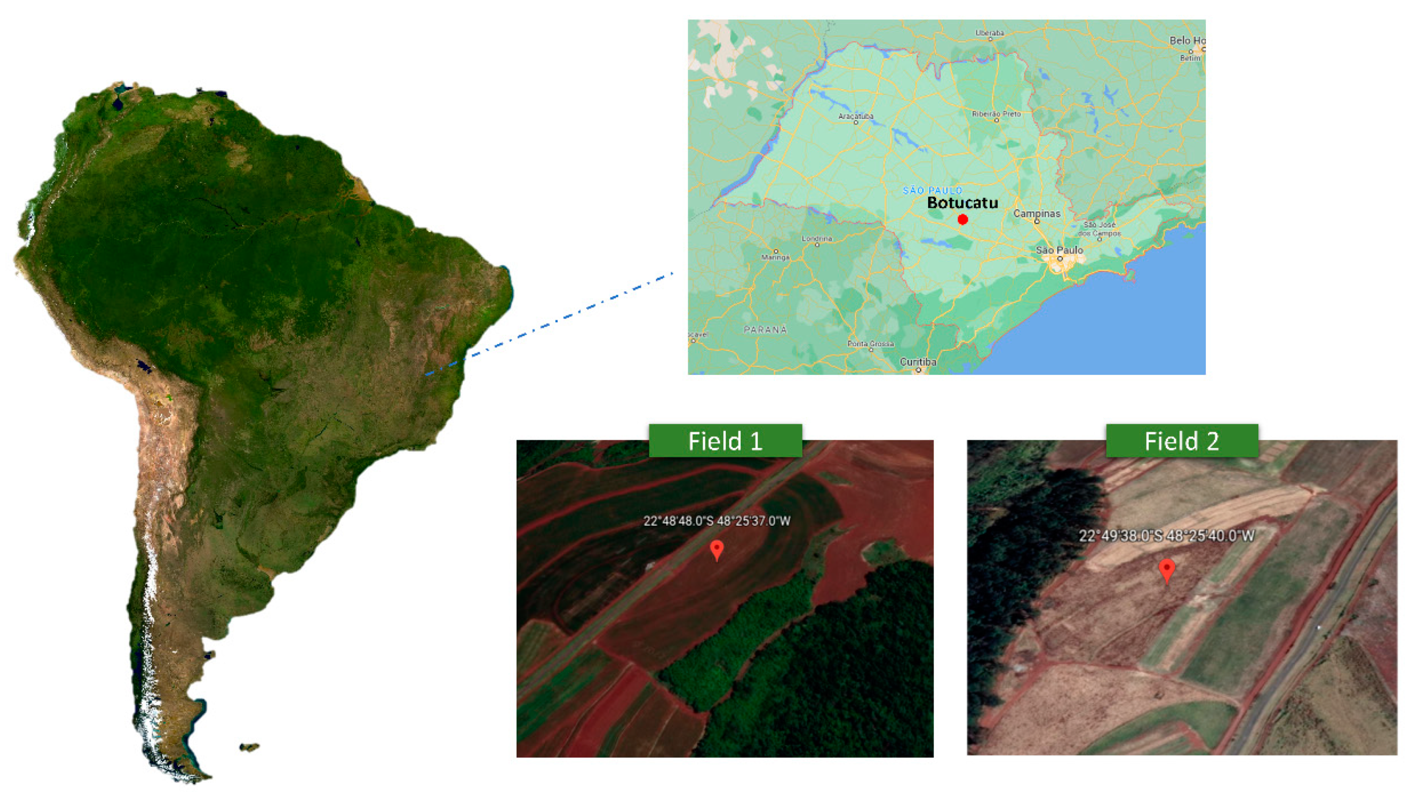
2. Materials and Methods
2.1. Leaf Reflectance Assessment
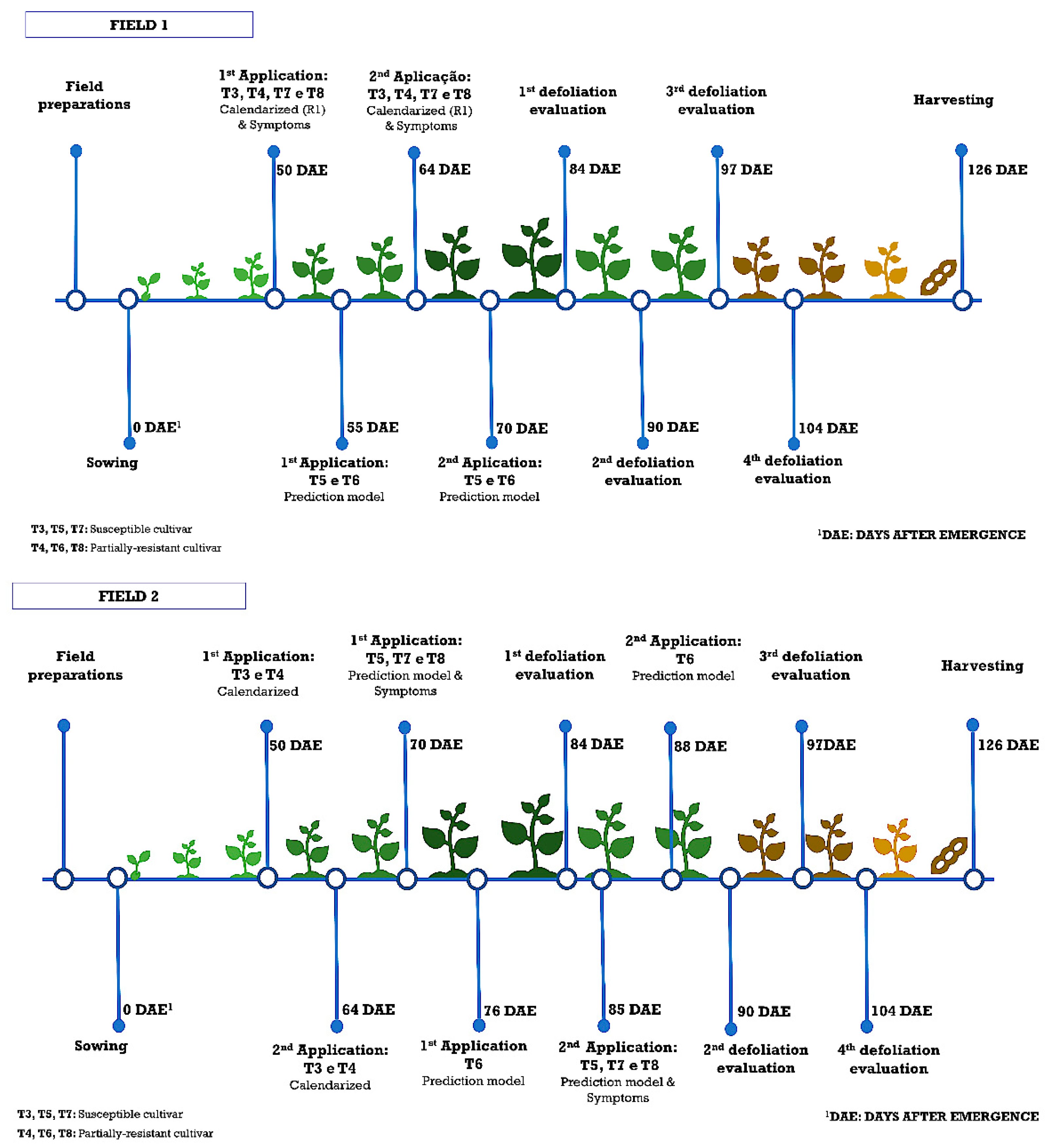
2.2. Fungicide Sprayings
2.3. Quali-Quantitative Analysis of Spraying
2.4. Assessment of Disease Severity and Control Efficacy
2.5. Evaluation of the Effect of Control on Crop Yield
2.6. Data Analysis
3. Results
3.1. Soybean Rust Detection and Application Timings
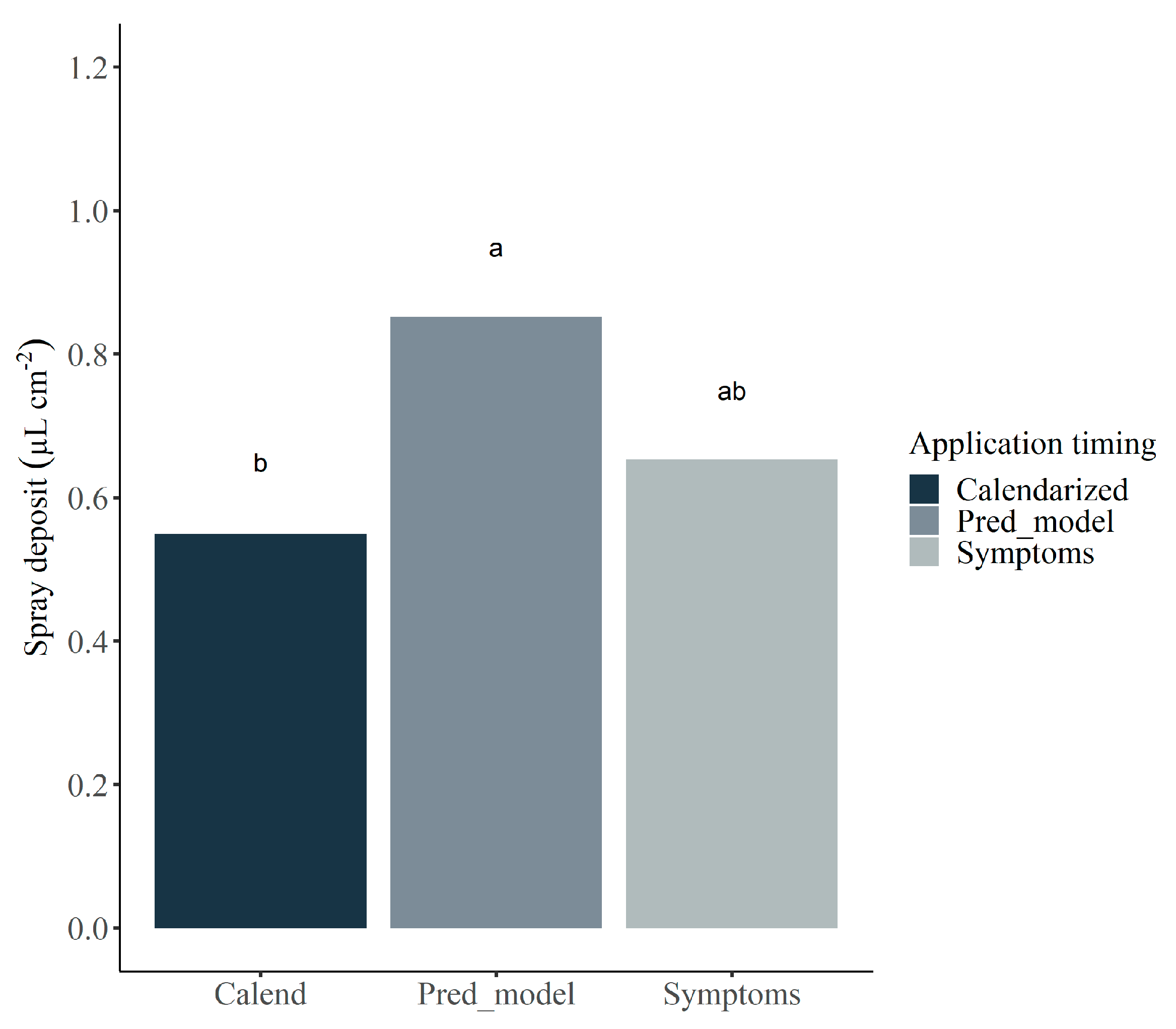
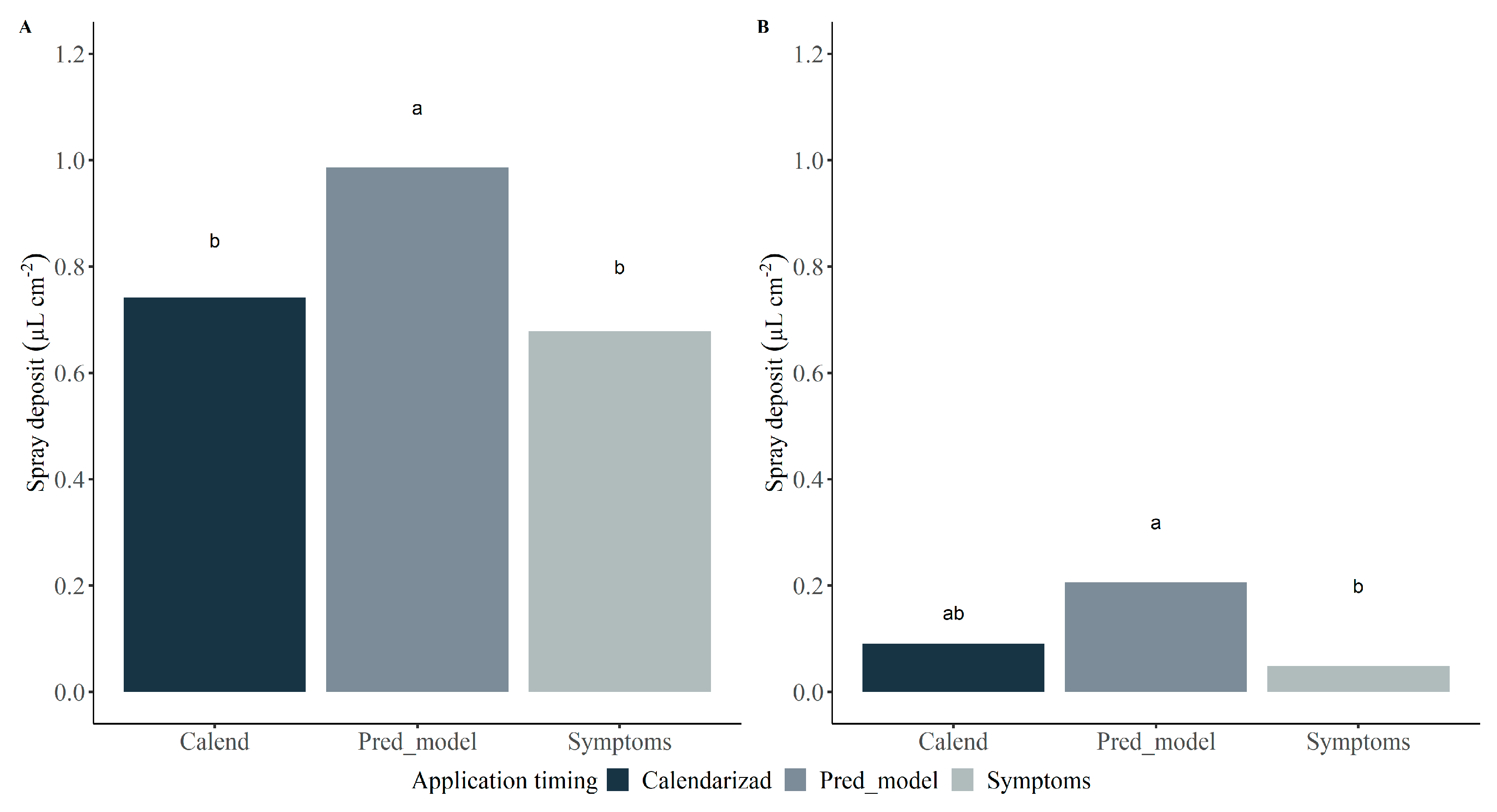
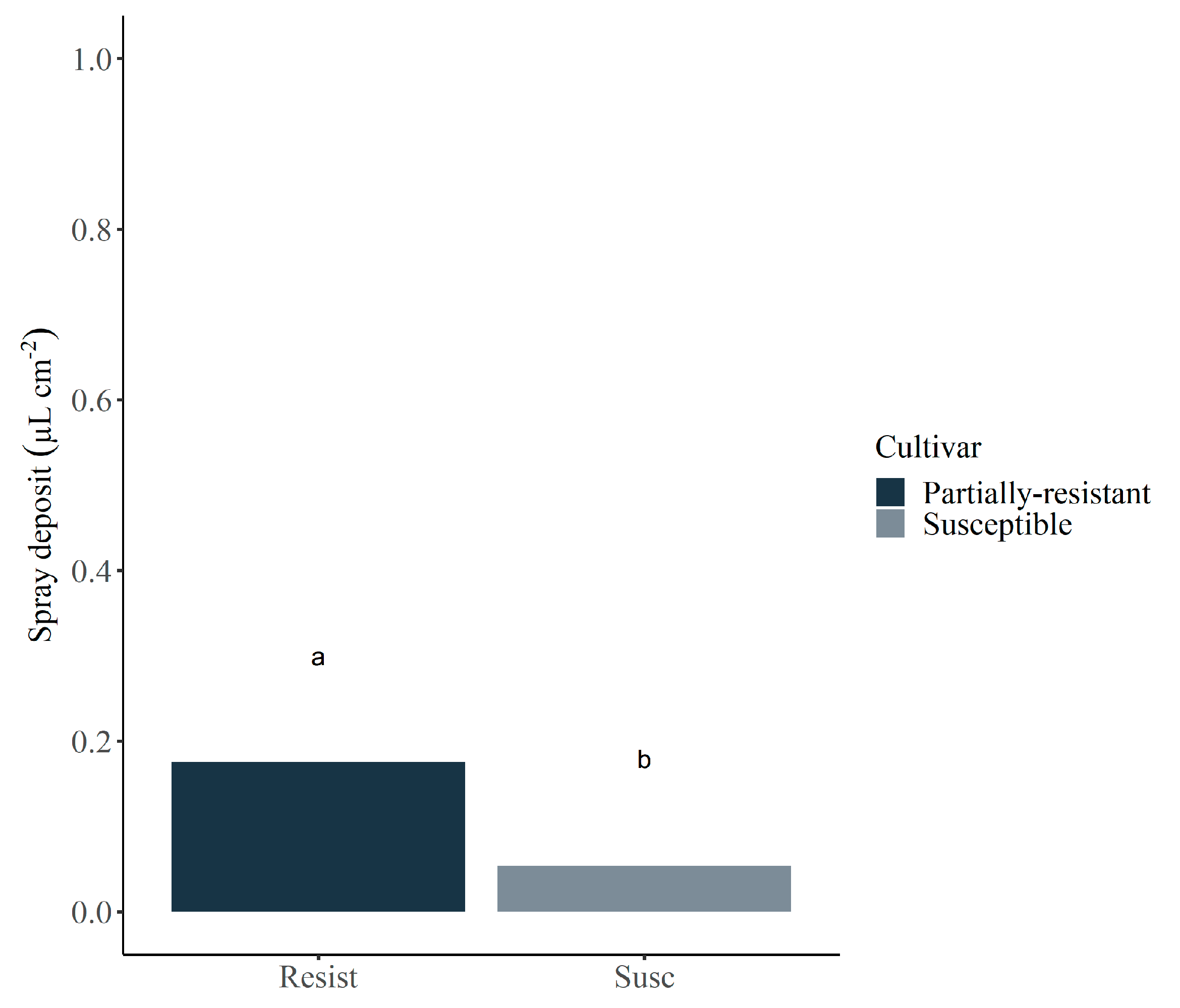
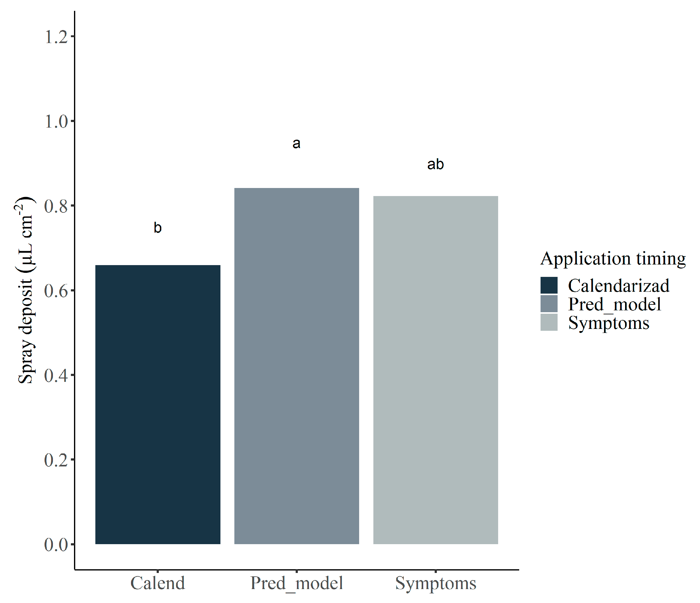
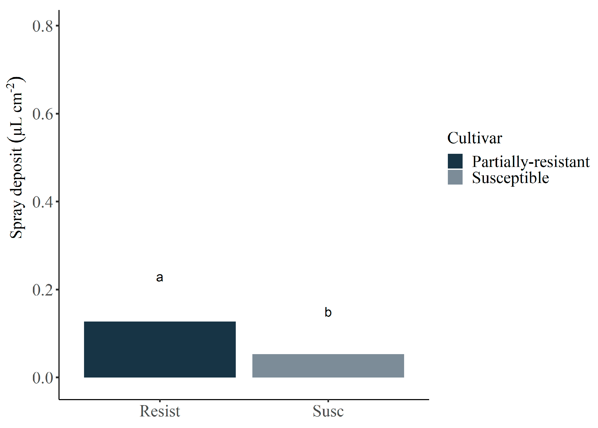
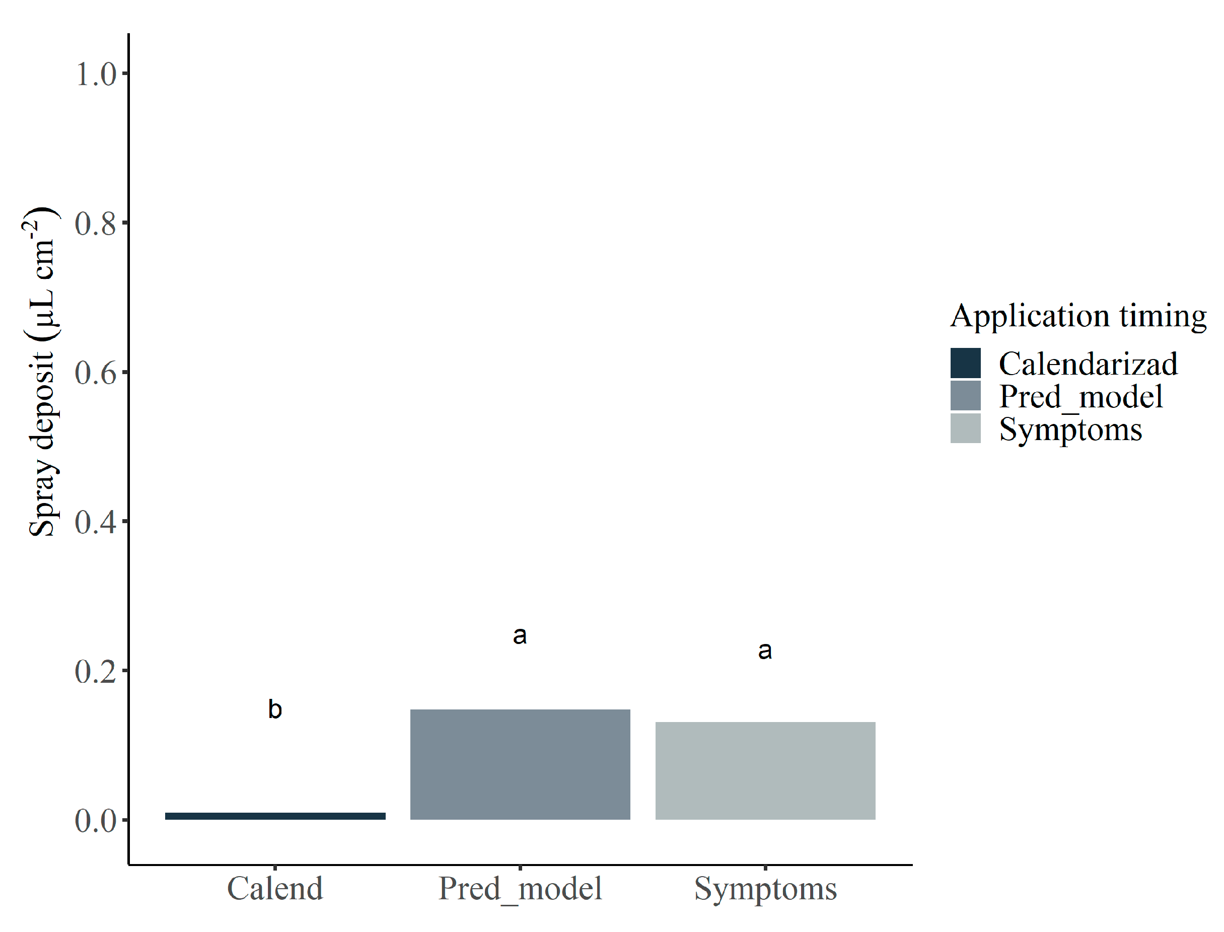
3.2. Spray Deposit
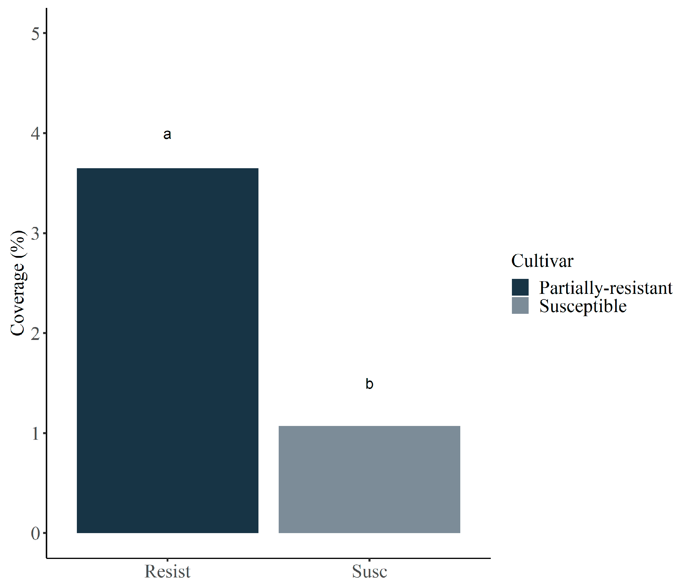
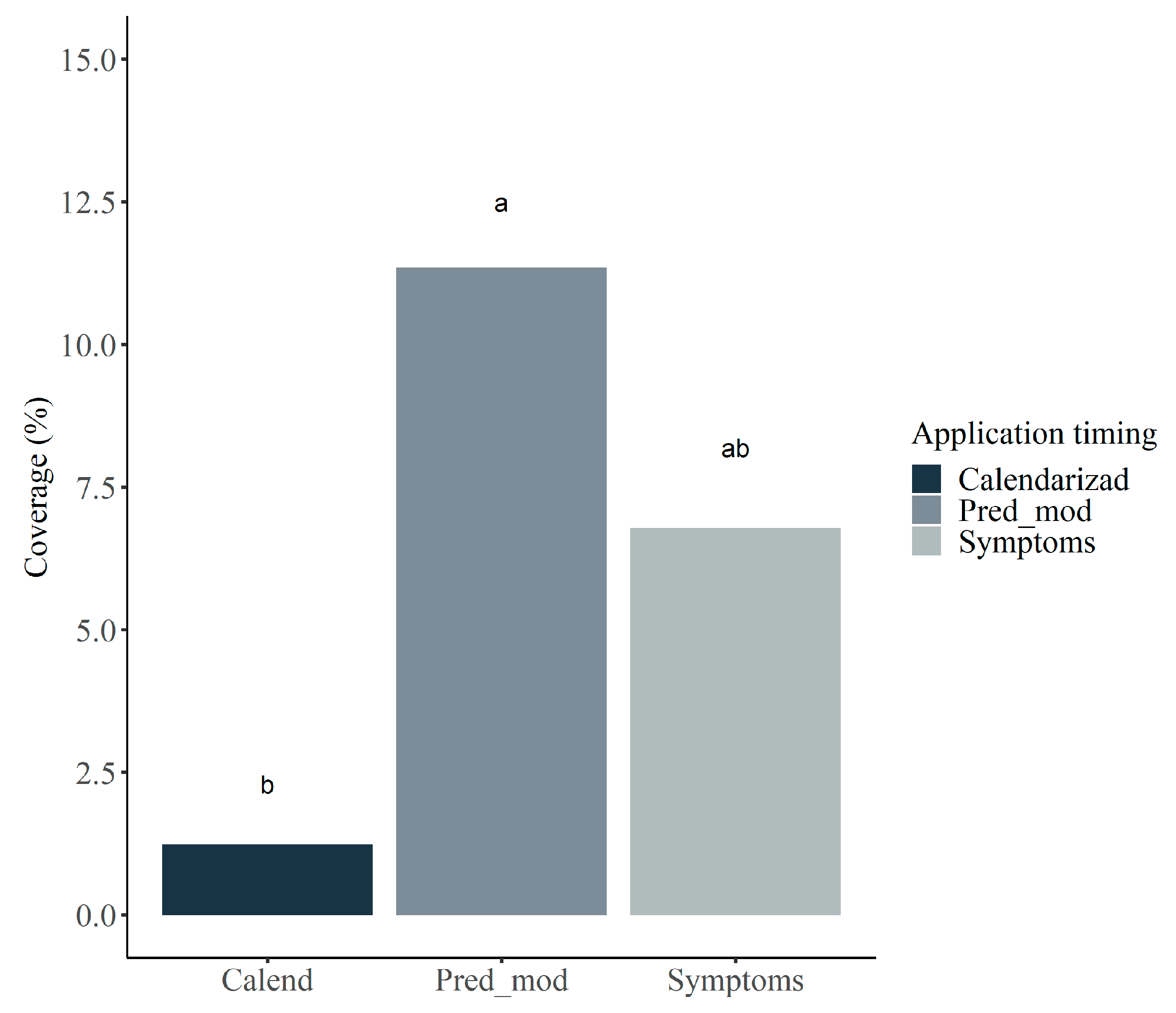
3.3. Spray Coverage
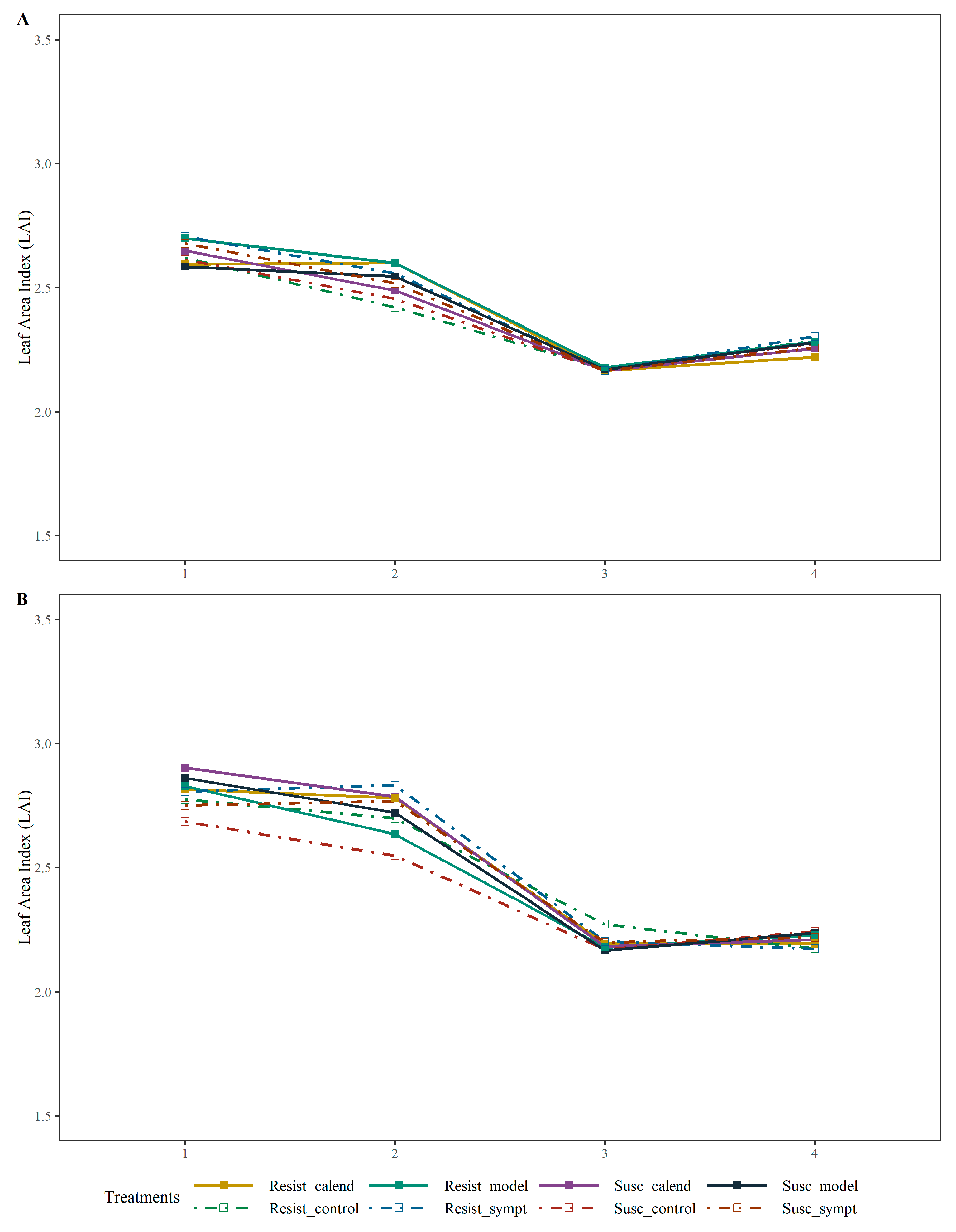
3.4. Effect of Application Timings on SBR Control and Crop Defoliation
3.5. Effect of SBR on Crop Yield
4. Discussion
Author Contributions
Funding
Institutional Review Board Statement
Informed Consent Statement
Data Availability Statement
Acknowledgments
Conflicts of Interest
References
- Godoy, C.V.; Seixas, C.D.S.; Soares, R.M.; Marcelino-Guimarães, F.C.; Meyer, M.C.; Costamilan, L.M. Asian soybean rust in Brazil: Past, present, and future. Pesqui. Agropecuária Bras. 2016, 51, 407–421. [Google Scholar] [CrossRef]
- Langenbach, C.; Campe, R.; Beyer, S.F.; Mueller, A.N.; Conrath, U. Fighting Asian soybean rust. Front Plant Sci. 2016, 7, 797. [Google Scholar] [CrossRef] [PubMed]
- Juliatti, F.C.; Azevedo, L.A.S.; Cristina, J. Strategies of chemical protection for controlling soybean rust. In Soybean; Kasai, M., Ed.; IntechOpen: London, UK, 2017; Volume 1, pp. 35–62. [Google Scholar]
- Hossain, M.M.; Yamanaka, N. Pathogenic variation of Asian soybean rust pathogen in Bangladesh. J. Gen. Plant Pathol. 2019, 85, 90–100. [Google Scholar] [CrossRef]
- Müller, M.A.; Stammler, G.; De Mio, L.L.M. Multiple resistance to DMI, QoI and SDHI fungicides in field isolates of Phakopsora pachyrhizi. Crop Prot. 2021, 145, 105618. [Google Scholar] [CrossRef]
- Dalla Lana, F.; Paul, P.A.; Godoy, C.V.; Utiamada, C.M.; da Silva, L.H.C.; Siqueri, F.V.; Forcelini, C.A.; Jaccoud-Filho, D.D.S.; Miguel-Wruck, D.S.; Borges, E.P.; et al. Meta-analytic modeling of the decline in performance of fungicides for managing soybean rust after a decade of use in Brazil. Plant Dis. 2018, 102, 807–817. [Google Scholar] [CrossRef]
- Ozkan, H.E.; Zhu, H.; Derksen, R.C.; Guler, H.; Krause, C. Evaluation of various spraying equipment for effective application of fungicides to control Asian soybean rust. Asp. Appl. Biol. 2006, 77, 423–431. [Google Scholar]
- Mueller, T.A.; Miles, M.R.; Morel, W.; Marois, J.J.; Wright, D.L.; Kemerait, R.C.; Hartman, G.L. Effect of fungicide and timing of application on soybean rust severity and yield. Plant Dis. 2009, 93, 243–248. [Google Scholar] [CrossRef]
- Cunha, J.P.A.R.; Juliatti, F.C.; Reis, E.F. Tecnologia de aplicação de fungicida no controle da ferrugem asiática da soja: Resultados de oito anos de estudos em minas gerais e goiás. Biosci. J. 2014, 30, 950–957. [Google Scholar]
- Hartman, G.L.; Miles, M.R.; Frederick, R.D. Breeding for resistance to soybean rust. Plant Dis. 2005, 89, 664–666. [Google Scholar] [CrossRef]
- Vittal, R.; Paul, C.; Hill, C.B.; Hartman, G.L. Characterization and quantification of fungal colonization of Phakopsora pachyrhizi in soybean genotypes. Phytopathology 2014, 104, 86–94. [Google Scholar] [CrossRef]
- Twizeyimana, M.; Hartman, G.L. Effect of selected biopesticides in reducing soybean rust (Phakopsora pachyrhizi) development. Plant Dis. 2019, 103, 2460–2466. [Google Scholar] [CrossRef] [PubMed]
- Corley, C.D.; Pullum, L.L.; Hartley, D.M.; Benedum, C.; Noonan, C.; Rabinowitz, P.M.; Lancaster, M.J. Disease prediction models and operational readiness. PLoS ONE 2014, 9, e91989. [Google Scholar] [CrossRef] [PubMed] [Green Version]
- Martinelli, F.; Scalenghe, R.; Davino, S.; Panno, S.; Scuderi, G.; Ruisi, P.; Dandekar, A.M. Advanced methods of plant disease detection. A review. Agron. Sustain. Dev. 2015, 35, 1–25. [Google Scholar] [CrossRef]
- Zhang, J.; Huang, Y.; Pu, R.; Gonzalez-Moreno, P.; Yuan, L.; Wu, K.; Huang, W. Monitoring plant diseases and pests through remote sensing technology: A review. Comput. Electron. Agric. 2019, 165, 104943. [Google Scholar] [CrossRef]
- Cui, D.; Zhang, Q.; Li, M.; Zhao, Y.; Hartman, G.L. Detection of soybean rust using a multispectral image sensor. Sens. Instrum. Food Qual. Saf. 2009, 3, 49–56. [Google Scholar] [CrossRef]
- Furlanetto, R.H.; Nanni, M.R.; Mizuno, M.S.; Crusciol, L.G.T.; da Silva, C.R. Identification and classification of Asian soybean rust using leaf-based hyperspectral reflectance. Int. J. Remote Sens. 2021, 42, 4177–4198. [Google Scholar] [CrossRef]
- Negrisoli, M.M.; Negrisoli, R.M.; da Silva, F.N.; Lopes, L.L.; Souza Júnior, F.S.; Velini, E.D.; Carbonari, C.A.; Rodrigues, S.A.; Raetano, C.G. Soybean rust detection and disease severity classification by remote sensing. Agron. J. 2022. [Google Scholar] [CrossRef]
- Bajwa, S.G.; Rupe, J.C.; Mason, J. Soybean disease monitoring with leaf reflectance. Remote Sens. 2017, 9, 127. [Google Scholar] [CrossRef]
- Donatelli, M.; Magarey, R.D.; Bregaglio, S.; Willocquet, L.; Whish, J.P.; Savary, S. Modelling the impacts of pests and diseases on agricultural systems. Agric. Syst. 2017, 155, 213–224. [Google Scholar] [CrossRef]
- Twizeyimana, M.; Hartman, G.L. Sensitivity of Phakopsora pachyrhizi isolates to fungicides and reduction of fungal infection based on fungicide and timing of application. Plant Dis. 2017, 101, 121–128. [Google Scholar] [CrossRef]
- Müller, M.; Rakocevic, M.; Caverzan, A.; Boller, W.; Chavarria, G. Architectural characteristics and heliotropism may improve spray droplet deposition in the middle and low canopy layers in soybean. Crop Sci. 2018, 58, 2029–2041. [Google Scholar] [CrossRef]
- Tagliapietra, E.L.; Streck, N.A.; Da Rocha, T.S.M.; Richter, G.L.; Da Silva, M.R.; Cera, J.C.; Guedes, J.V.C.; Zanon, A.J. Optimum leaf area index to reach soybean yield potential in subtropical environment. Agron. J. 2018, 10, 932–938. [Google Scholar] [CrossRef] [Green Version]
- Negrisoli, M.M.; Raetano, C.G.; de Souza, D.M.; Souza, F.M.S.; Bernardes, L.M.; Junior, L.D.B.; Rodrigues, D.M.; Sartori, M.M.P. Performance of new flat fan nozzle design in spray deposition, penetration and control of soybean rust. Eur. J. Plant Pathol. 2019, 155, 755–767. [Google Scholar] [CrossRef]
- Brevant Sementes—Cultivares de Soja: DS6217IPRO. Available online: https://www.brevant.com.br/produtos/soja/ds6217ipro.html (accessed on 26 January 2022).
- Tropical Melhoramento Genético (TMG)—Cultivares de Soja: TMG 7063 IPRO. Available online: http://www.tmg.agr.br/ptbr/cultivar/tmg-7063-ipro (accessed on 26 January 2022).
- Abdel-Rahman, E.M.; Mutanga, O.; Odindi, J.; Adam, E.; Odindo, A.; Ismail, R. A comparison of partial least squares (PLS) and sparse PLS regressions for predicting yield of Swiss chard grown under different irrigation water sources using hyperspectral data. Comput. Electron. Agric. 2014, 106, 11–19. [Google Scholar] [CrossRef]
- Savitzky, A.; Golay, M.J. Smoothing and differentiation of data by simplified least squares procedures. Analytical. Chem. 1964, 36, 1627–1639. [Google Scholar] [CrossRef]
- Bohnenkamp, D.; Behmann, J.; Mahlein, A.K. In-field detection of yellow rust in wheat on the ground canopy and UAV scale. Remote Sens. 2019, 11, 2495. [Google Scholar] [CrossRef]
- Abdi, H.; Williams, L.J.; Valentin, D. Multiple factor analysis: Principal component analysis for multitable and multiblock data sets. Wiley Interdiscip. Rev. Comput. Stat. 2013, 5, 149–179. [Google Scholar] [CrossRef]
- Palladini, L.A.; Raetano, C.G.; Velini, E.D. Choice of tracers for the evaluation of spray deposits. Sci. Agric. 2005, 62, 440–445. [Google Scholar] [CrossRef]
- Jonckheere, I.; Fleck, S.; Nackaerts, K.; Muys, B.; Coppin, P.; Weiss, M.; Baret, F. Review of methods for in situ leaf area index determination: Part I. Theories, sensors and hemispherical photography. Agric. For. Meteorol. 2004, 121, 19–35. [Google Scholar] [CrossRef]
- Godoy, C.V.; Koga, L.J.; Canteri, M.G. Diagrammatic scale for assessment of soybean rust severity. Fitopatol. Bras. 2006, 31, 63–68. [Google Scholar] [CrossRef]
- Campbell, C.L.; Madden, L.V. Introduction to Plant Disease Epidemiology; John Wiley & Sons: New York, NY, USA, 1994; 532p. [Google Scholar]
- Tan, C.W.; Zhang, P.P.; Zhou, X.X.; Wang, Z.X.; Xu, Z.Q.; Mao, W.; Yun, F. Quantitative monitoring of leaf area index in wheat of different plant types by integrating NDVI and Beer-Lambert law. Sci. Rep. 2020, 10, 1–10. [Google Scholar] [CrossRef] [PubMed]
- Brasil. Ministério da Agricultura, Pecuária e Abastecimento. Regras Para Análise de Sementes; Ministério da Agricultura, Pecuária e Abastecimento—Secretaria de Defesa Agropecuária: Brasília, Brazil, 2009; 395p.
- R Core Team. R: A Language and Environment for Statistical Computing; R Foundation for Statistical Computing: Vienna, Austria, 2013. [Google Scholar]
- Kelly, H.Y.; Dufault, N.S.; Walker, D.R.; Isard, S.A.; Schneider, R.W.; Giesler, L.J.; Hartman, G.L. From select agent to an established pathogen: The response to Phakopsora pachyrhizi (soybean rust) in North America. Phytopathology 2015, 105, 905–916. [Google Scholar] [CrossRef] [PubMed] [Green Version]
- Berger-Neto, A.; Jaccoud-Filho, D.S.; Wutzki, C.R.; Tullio, H.E.; Pierre, M.L.C.; Manfron, F.; Justino, A. Effect of spray droplet size, spray volume and fungicide on the control of white mold in soybeans. Crop Prot. 2017, 92, 190–197. [Google Scholar] [CrossRef]
- Balardin, R.; Madalosso, M.; Debortoli, M.; Lenz, G. Factors affecting fungicide efficacy in the tropics. In Fungicides; Carisse, O., Ed.; InTech Open: London, UK, 2010; pp. 23–38. [Google Scholar]
- Van Den Bosch, F.; Paveley, N.; Shaw, M.; Hobbelen, P.; Oliver, R. The dose rate debate: Does the risk of fungicide resistance increase or decrease with dose? Plant Pathol. 2011, 60, 597–606. [Google Scholar] [CrossRef]
- Ferguson, J.C.; Hewitt, A.J.; O’Donnell, C.C. Pressure, droplet size classification, and nozzle arrangement effects on coverage and droplet number density using air-inclusion dual fan nozzles for pesticide applications. Crop Prot. 2016, 89, 231–238. [Google Scholar] [CrossRef]
- Sharpe, S.M.; Boyd, N.S.; Dittmar, P.J.; Macdonald, G.E.; Darnell, R.L.; Ferrel, J.A. Spray penetration into a strawberry canopy as affected by canopy structure, nozzle type, and application volume. Weed Technol. 2017, 32, 80–84. [Google Scholar] [CrossRef]
- Childs, S.P.; Buck, J.W.; Li, Z. Breeding soybeans with resistance to soybean rust (Phakopsora pachyrhizi). Plant Breed. 2018, 137, 250–261. [Google Scholar] [CrossRef]
- Hartman, G.L.; Hill, C.B.; Twizeyimana, M.; Miles, M.R.; Bandyopadhyay, R. Interaction of soybean and Phakopsora pachyrhizi, the cause of soybean rust. CAB Rev. Perspect. Agric. Vet. Sci. Nutr. Nat. Resour. 2011, 6, 59. [Google Scholar] [CrossRef]
- Verreet, J.A.; Klink, H.; Hoffmann, G.M. Regional monitoring for disease prediction and optimization of plant protection measuares: The IPM wheat model. Plant Dis. 2000, 84, 816–826. [Google Scholar] [CrossRef]
- Sapak, Z.; Salam, M.U.; Minchinton, E.J.; MacManus, G.P.V.; Joyce, D.C.; Galea, V.J. POMICS: A simulation disease model for timing fungicide applications in management of powdery mildew of cucurbits. Phytopathology 2017, 107, 1022–1031. [Google Scholar] [CrossRef]
- Gama, A.B.; Peres, N.A.; Singerman, A.; Dewdney, M.M. Evaluation of disease alert systems for postbloom fruit drop of citrus in Florida and economic impact of adopting the Citrus Advisory System. Crop Prot. 2022, 155, 105906. [Google Scholar] [CrossRef]
- Yuan, H.; Yang, G.; Li, C.; Wang, Y.; Liu, J.; Yu, H.; Yang, X. Retrieving soybean leaf area index from unmanned aerial vehicle hyperspectral remote sensing: Analysis of RF, ANN, and SVM regression models. Remote Sens. 2017, 9, 309. [Google Scholar] [CrossRef] [Green Version]
- Kawuki, R.S.; Tukamuhabwa, P.; Adipala, E. Soybean rust severity, rate of rust development, and tolerance as influenced by maturity period and season. Crop Prot. 2004, 23, 447–455. [Google Scholar] [CrossRef]
- Kumudini, S.; Prior, E.; Omielan, J.; Tollenaar, M. Impact of Phakopsora pachyrhizi infection on soybean leaf photosynthesis and radiation absorption. Crop Sci. 2008, 48, 2343–2350. [Google Scholar] [CrossRef] [Green Version]


| Treatments | Cultivar | First Application Timing | Second Application Timing |
|---|---|---|---|
| 1 | DS6217 IPRO (Susceptible) | - | - |
| 2 | TMG 7063 (Partially resistant) | - | - |
| 3 | DS6217 IPRO (Susceptible) | Calend * | Calend + 15 |
| 4 | TMG 7063 (Partially resistant) | Calend | Calend + 15 |
| 5 | DS6217 IPRO (Susceptible) | Model | Model + 15 |
| 6 | TMG 7063 (Partially resistant) | Model | Model + 15 |
| 7 | DS6217 IPRO (Susceptible) | Sympt | Sympt + 15 |
| 8 | TMG 7063 (Partially resistant) | Sympt | Sympt + 15 |
| Description | Brevant DS6217 IPRO 1 | TMG 7063 2 |
|---|---|---|
| P. pachyrhizi susceptibility | Susceptible | Partially resistant (Inox) |
| Maturity groups | 6.2 | 6.3 |
| Growth habit | Indeterminate | Indeterminate |
| Traits | Intacta RR2 PRO® | Intacta RR2 PRO® |
| Application Timing | Cultivar | |
|---|---|---|
| Susceptible | Partially Resistant | |
| Calendarized | 5.14 aB | 21.97 aA |
| Prediction model | 6.57 aA | 2.06 bA |
| Symptoms | 6.74 aA | 4.27 bA |
| Cause of Variation | F | P |
| Application timing (AT) | 2.885 | 0.087 NS |
| Cultivar © | 0.922 | 0.352 NS |
| AT x C | 3.958 | 0.042 * |
| Field | Application Timing | AUDPC | Control (%) | ||
|---|---|---|---|---|---|
| Cultivar | Cultivar | ||||
| Susceptible | P. Resistant | Susceptible | P. Resistant | ||
| Field 1 | Control | 200.80 aA | 40.50 aB | - | - |
| Calendarized | 68.90 bA | 18.10 aB | 64.40 | 51.50 | |
| Prediction model | 54.60 bA | 15.90 aB | 71.60 | 59.20 | |
| Symptoms | 63.00 bA | 15.00 aB | 67.90 | 58.90 | |
| Causes of Variation | F | P | F | P | |
| App. Timing (AT) | 53.450 | <0.001 *** | 0.576 | 0.574 NS | |
| Cultivar © | 177.450 | <0.001 *** | 3.772 | 0.071 NS | |
| AT x C | 26.450 | <0.001 *** | 0.042 | 0.959 NS | |
| Field 2 | Control | 519.20 aA | 65.70 aB | - | - |
| Calendarized | 138.90 bA | 32.50 aB | 72.50 aA | 47.80 bB | |
| Prediction model | 142.50 bA | 22.40 aB | 71.70 aA | 65.70 aA | |
| Symptoms | 191.00 bA | 27.10 aB | 62.10 aA | 56.74 abA | |
| Causes of Variation | F | P | F | P | |
| App. timing (AT) | 43.076 | <0.001 *** | 143.823 | <0.001 *** | |
| Cultiv©(C) | 188.949 | <0.001 *** | 8.577 | 0.008 * | |
| AT x C | 28.402 | <0.001 *** | 5.019 | 0.009 * | |
| Application Timing | Crop Yield | TSW | ||
|---|---|---|---|---|
| kg ha−1 | g | |||
| Field 1 | Field 2 | Field 1 | Field2 | |
| Control | 2393.714 | 2799.833 b | 2393.71 | 2799.83 b |
| Calendarized | 3143.054 | 3462.89 a | 3143.05 | 3462.89 a |
| Prediction model | 2738.061 | 3055.73 ab | 2738.06 | 3055.73 ab |
| Symptoms | 2817.034 | 3169.037 ab | 2817.03 | 3169.04 ab |
| F value | 2.713 NS | 4.092 * | 5.510 *** | 1.804 NS |
| CV (%) | 19.05 | 12.31 | 6.47 | 8.54 |
Publisher’s Note: MDPI stays neutral with regard to jurisdictional claims in published maps and institutional affiliations. |
© 2022 by the authors. Licensee MDPI, Basel, Switzerland. This article is an open access article distributed under the terms and conditions of the Creative Commons Attribution (CC BY) license (https://creativecommons.org/licenses/by/4.0/).
Share and Cite
Negrisoli, M.M.; Silva, F.N.d.; Negrisoli, R.M.; Lopes, L.d.S.; Souza Júnior, F.d.S.; Freitas, B.R.d.; Velini, E.D.; Raetano, C.G. Impact of Fungicide Application Timing Based on Soybean Rust Prediction Model on Application Technology and Disease Control. Agronomy 2022, 12, 2119. https://doi.org/10.3390/agronomy12092119
Negrisoli MM, Silva FNd, Negrisoli RM, Lopes LdS, Souza Júnior FdS, Freitas BRd, Velini ED, Raetano CG. Impact of Fungicide Application Timing Based on Soybean Rust Prediction Model on Application Technology and Disease Control. Agronomy. 2022; 12(9):2119. https://doi.org/10.3390/agronomy12092119
Chicago/Turabian StyleNegrisoli, Matheus Mereb, Flávio Nunes da Silva, Raphael Mereb Negrisoli, Lucas da Silva Lopes, Francisco de Sales Souza Júnior, Bianca Rezende de Freitas, Edivaldo Domingues Velini, and Carlos Gilberto Raetano. 2022. "Impact of Fungicide Application Timing Based on Soybean Rust Prediction Model on Application Technology and Disease Control" Agronomy 12, no. 9: 2119. https://doi.org/10.3390/agronomy12092119
APA StyleNegrisoli, M. M., Silva, F. N. d., Negrisoli, R. M., Lopes, L. d. S., Souza Júnior, F. d. S., Freitas, B. R. d., Velini, E. D., & Raetano, C. G. (2022). Impact of Fungicide Application Timing Based on Soybean Rust Prediction Model on Application Technology and Disease Control. Agronomy, 12(9), 2119. https://doi.org/10.3390/agronomy12092119