Article

Use of Active Sensors in Coffee Cultivation for Monitoring Crop Yield

by
Maurício Martello
1,*,
José Paulo Molin
1,
Helizani Couto Bazame
1,
Tiago Rodrigues Tavares
2 and
Leonardo Felipe Maldaner
1
1
Laboratory of Precision Agriculture (LAP), Department of Biosystems Engineering, “Luiz de Queiroz” College of Agriculture (ESALQ), University of São Paulo (USP), Piracicaba 13418-900, Brazil
2
Laboratory of Nuclear Instrumentation (LIN), Center for Nuclear Energy in Agriculture (CENA), University of São Paulo (USP), Piracicaba 13416-000, Brazil
*
Author to whom correspondence should be addressed.
Agronomy 2022, 12(9), 2118; https://doi.org/10.3390/agronomy12092118
Submission received: 13 August 2022 / Revised: 25 August 2022 / Accepted: 29 August 2022 / Published: 7 September 2022
(This article belongs to the Section Precision and Digital Agriculture)

Abstract

:
Monitoring the spatial variability of agricultural variables is a main step in implementing precision agriculture practices. Active optical sensors (AOS), with their instrumentation directly on agricultural machines, are suitable and make it possible to obtain high-frequency data. This study aimed to evaluate the potential of AOS to map the spatial and temporal variability of coffee crop yields, as well as to establish guidelines for the acquisition of AOS data for sensing the sides of a coffee plant, allowing the evaluation of large commercial fields. The study was conducted in a commercial coffee area of 10.24 ha, cultivated with the Catuaí 144 variety. Data collection was performed with six Crop Circle ACS 430 sensors (Holland Scientific, Lincoln, NE, USA) and two N-Sensor NG sensors (Yara International, Dülmen, Germany). Seven field expeditions were made to collect data using the optical sensors during 2019 and 2021, obtaining data during the flowering, fruit-filling and fruit maturation phases (pre-harvest), and post-harvest. The results showed that the different faces of the same plant present a different Pearson’s correlation coefficient (r) to its yield, obtained with a yield monitor on the harvester. The face with the highest exposure to solar radiation presented a slightly higher correlation to yield (−0.34 ≤ r ≤ −0.17) when compared with the face with less exposure (−0.27 ≤ r ≤ −0.15). In addition, it was observed that the vegetation indices measured at the beginning of the coffee cycle (before the rainy season that starts in October) present a positive correlation to the coffee yield of that same year (0.73 ≤ r ≤ 0.91). On the other hand, this relationship is changed after the beginning of the rain season, at which time the vegetation index increases abruptly, inverting the correlation with the yield after that (−0.93 ≤ r ≤ −0.77). Furthermore, it was observed that, due to the biennial nature of coffee production, the vegetation index acquired at a specific time has an inverted relationship when compared with the yield of that year and to the yield of the following (or previous) year.

1. Introduction

Precision Agriculture (PA) approaches seek to understand the spatial and temporal variability present in agricultural variables within a production field. This knowledge allows for the localized management of inputs, aiming to increase production efficiency and, therefore, the profitability and sustainability of agricultural production [1]. Monitoring the spatial variability of agricultural variables is a main step in implementing PA techniques. This step routinely demands a high spatial density of data for the construction of reliable maps that characterize details of the crop. In addition, monitoring large-scale crops (e.g., hundreds of hectares) requires practical, inexpensive technologies that are compatible with the automation of the monitoring process.
Remote-sensing approaches (e.g., remotely piloted aircraft images) are classic alternatives for monitoring agricultural variables on large tracts of land, allowing spatial resolution from a few meters (e.g., 2–30 m for satellite images) up to sub-metric values. On the other hand, proximal sensing using active optical sensors (AOS) with instrumentation directly on agricultural machines is suitable and allows high-frequency data (e.g., 5 Hz) to be obtained, which amounts to more than one piece of information per plant. In addition, as the sensors are active, they do not depend on external radiation sources. AOS are less affected by variability in lighting and shading, which is common in field data acquisition, e.g., the presence of clouds or variation in solar position, factors to consider when using orbital and aerial remote-sensing approaches.
In agriculture, AOS were initially developed to identify changes in nitrogen (N) nutritional status and estimate its demand. This is possible because these sensors are able to monitor the photosynthetic activity and vegetative vigor of plants, both factors being related to N absorption in most crops [2]. An advantage of these sensors is that they do not depend on post-processing steps, as do imaging sensors. This allows the synchronization of collection, diagnosis, prescription and application in one single step, making real-time interventions possible [3]. Studies were already developed using AOS for crops, such as maize [4,5,6,7], wheat [8,9,10,11], rice [12], cotton [13] and sugarcane [14,15,16]. However, these approaches were not explored in depth for coffee cultivation, with only a few scientific studies evaluating the performance of AOS to estimate biometric parameters of individual plants [17,18] and are, therefore, not applicable to large-scale contexts, such as in commercial areas.
Unlike annual crops, active optical sensing for coffee should be performed with equipment turned to the side view of the plants, since positioning the sensor at the top of the plant is unfeasible due to the canopy height. Although the lateral positioning of active sensors was already adopted in some studies monitoring perennial crops [19,20,21], there is still a need to establish an optimized protocol for the acquisition and processing of these data for coffee crops in order to evaluate its spatial variability over its biennial cycle. For example, in crops with planting lines oriented in an east–west direction, there is no consensus on using data from only one of the side faces (i.e., using only the face that does not receive direct sunlight) or whether the best strategy is to use a methodology to calculate the average of both faces. This fact must be considered as there is a consensus that the face receiving more solar radiation behaves differently, resulting in different vegetative vigor when the same plant is evaluated from opposite faces/sides [22,23,24,25,26,27]. It is not known, therefore, which of these faces best represents the crop’s yield potential. In addition, neither is there any consensus on which part of the coffee plants, i.e., middle, lower, or upper third, should be scanned to obtain data that best represent the variability of this crop. Finally, it is important to mention that, to the best of our knowledge, there is no long-term research evaluating the response of AOS in the coffee crop over the biennial cycle typical of this crop.
In this context, this study aimed to evaluate the potential of AOS to map the spatial and temporal variability of coffee crop yields, allowing the evaluation of large commercial fields. More specifically, this study (i) evaluates and proposes a strategy for acquiring AOS data from the side of coffee plants and (ii) assesses the spatial relationship between data from different commercial AOS and coffee yield, evaluating the crop over its biennial cycle.

2. Materials and Methods
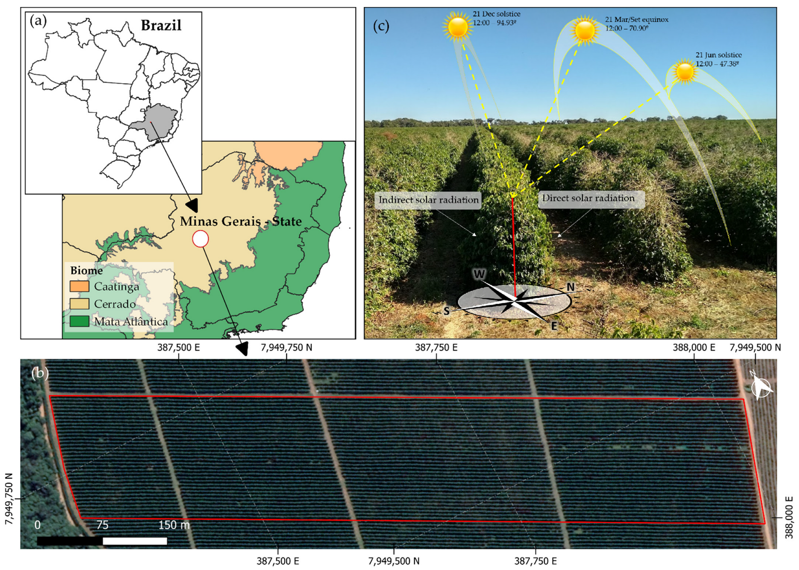
2.1. Study Area

The study was conducted in a commercial coffee area of 10.24 ha, cultivated with the Catuaí 144 variety. The coffee trees were spaced at 0.5 m between plants and 4.0 m between rows, resulting in a density of approximately 5000 plants ha−1, with a drip irrigation system. The area (Figure 1) is located in the municipality of Patos de Minas, state of Minas Gerais, Brazil. The local climate is classified as Aw (Tropical savanna climate), according to the Köppen classification [28], characterized by a tropical environment with dry winters and rainy summers. The coffee lines were planted in an east–west direction so that one side of the plants received direct solar radiation most of the year and the other side received indirect radiation (Figure 1a).

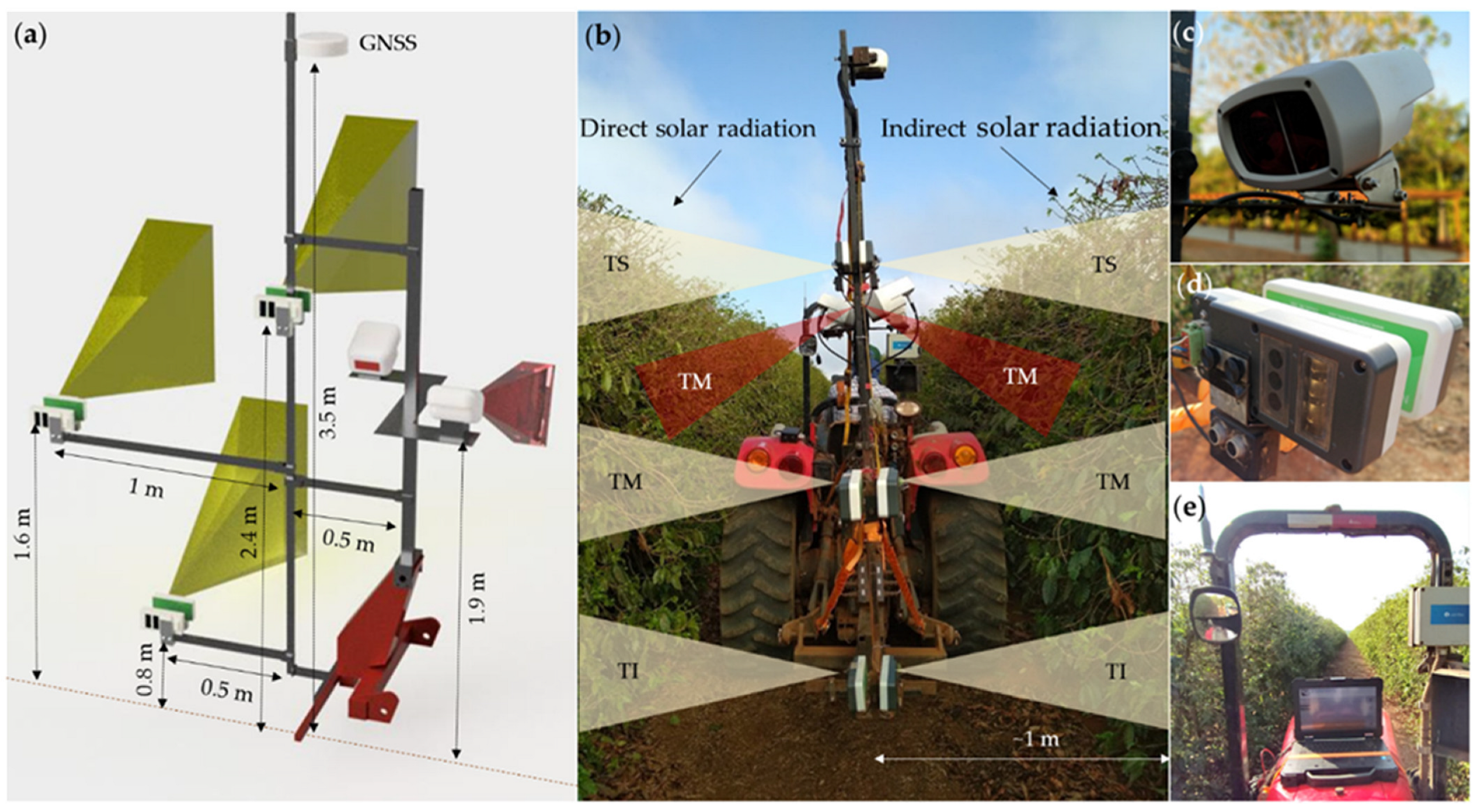
2.2. Tractor Instrumentation with AOS

Data collection was performed with six Crop Circle ACS 430 sensors (Holland Scientific, Lincoln, NE, USA) and two N-Sensor NG sensors (Yara International, Dülmen, Germany). The sensors were embedded in an agricultural tractor. Sensor specifications are shown in Table 1. The arrangement of sensors on the machine was previously defined in a 3D environment to avoid overlapping the lighting emitted by the active sensors (Figure 2a). Details of sensor positioning are shown in Figure 2.
The Crop Circle sensors were positioned at three different heights to simultaneously scan the lower (0 to 0.8 m, designated as TI), middle (0.8 to 1.6 m, designated as TM) and upper (1.6 to 2.4 m, designated as TS) thirds of the coffee plants. The N-Sensor sensors were positioned to scan only the middle third of the coffee plants. Half of the sensors collected data from the right row and the other half from the left row, with the tractor moving between the coffee rows. All equipment worked with a data acquisition frequency of 5 Hz, obtaining approximately 1 point on each side of the plant every 0.3 m (considering an average traveling speed of 1.5 m s−1).
The Crop Circle sensors were integrated with the GEOSCOUT GLS-420 mapping system (Holland Scientific, Lincoln, NE, USA) for data acquisition, and the NDVI (Normalized Difference Vegetation Index) [29] and NDRE (normalized difference red edge index) [30] vegetation indices were calculated, being designated in this study as CC-NDVI and CC-NDRE, respectively. The N-Sensor data acquisition was made in Yara N-Sensor software running on the Microsoft Windows operating system. The sensor provides a vegetation index (designated in this work as NS), for which the company does not disclose specifications. All data were georeferenced using a Global Navigation Satellite System (GNSS) receiver (SMART6-L™, NovAtel Inc., Calgary, AB, Canada) with TerraStar-C (NovAtel Inc., Calgary, AB, Canada) correction that allows an accuracy of ±0.09 m [31].

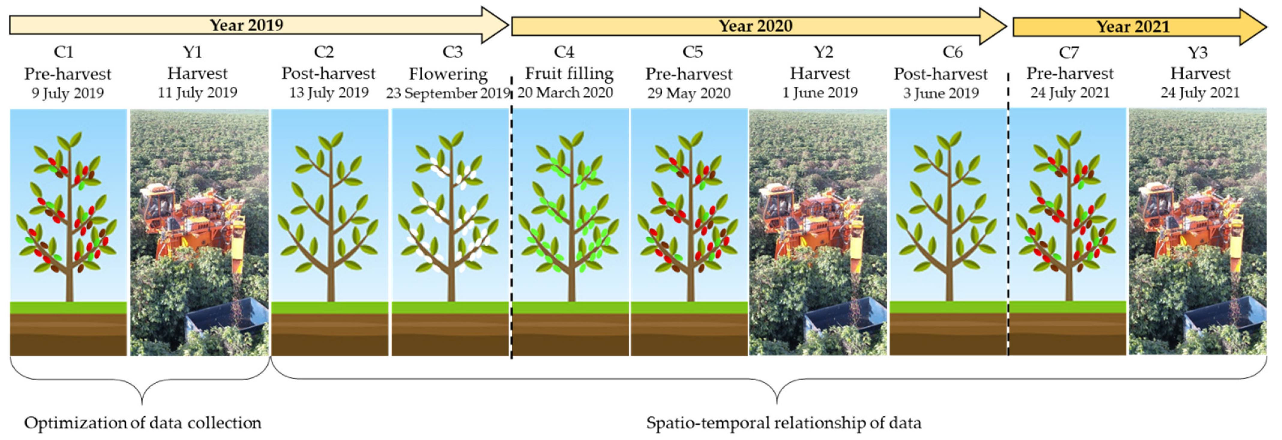
2.3. Data Acquisition with AOS and Yield Measurement

Seven field expeditions (designated from C1 to C7) were made for data collection with the optical sensors during the years 2019 to 2021 (Figure 3), collecting data during the flowering, fruit-filling and fruit maturation phases (pre-harvest), and post-harvest. Harvests were carried out in 2019, 2020 and 2021 using a K3 Millennium harvester (Jacto, Pompeia, Brazil), equipped with a yield monitor that measures the volume of harvested grains converted to weight using a conversion factor. More details of the yield monitor and the conversion from volumetric to gravimetric units are described by Martello et al. [32]. Yield data collected from maneuvers and roads were manually removed. Subsequently, the discrepant data were filtered using the software MapFilter V.2.0 (Piracicaba, Brazil) [33], using global filtering with a threshold of 100% [34].

2.4. Data Analysis

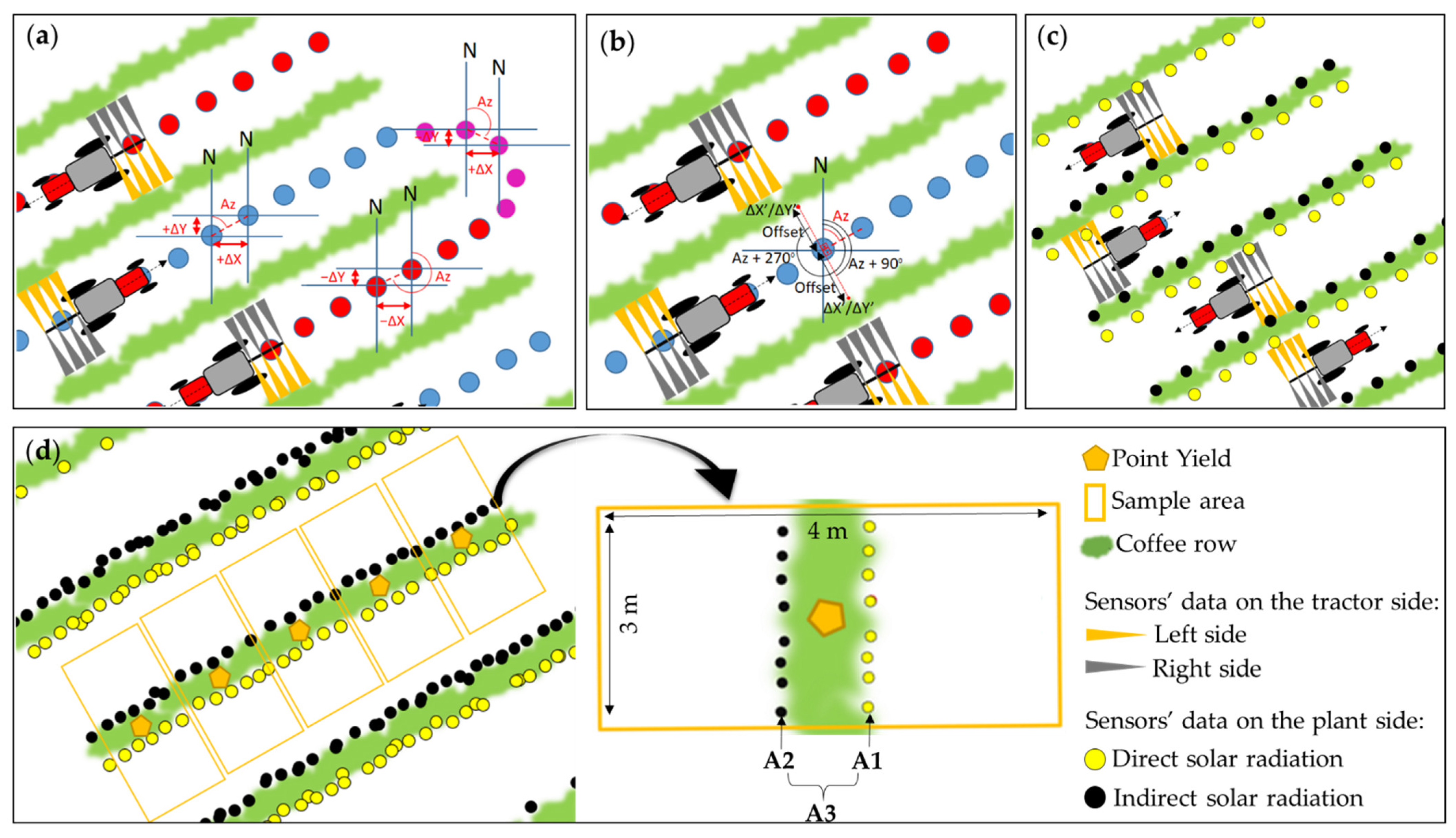
2.4.1. Optimizing AOS Positioning on the Side of a Coffee Plant to Infer Its Yield

Three data acquisition scenarios were evaluated: (i) using only data obtained on the face exposed to direct sunlight (A1); (ii) using only the data obtained on the face with indirect sun exposure (A2); and (iii) using the average of the two faces for the same plant (A3). To categorize the sensor data as a function of the face exposed to direct or indirect sunlight, an algorithm was developed that recognized the direction of the tractor’s displacement as a function of the azimuth of its coordinates. The points were classified according to the direction of the tractor displacement (Figure 4a) and an offset of 2 m was then applied to reproject the position to the center of the row at 90° and 270° from the alignment (Figure 4b). This was necessary because the equipment positioned to the right and left of the tractor scans different faces as the direction of displacement is reversed.
The optimization of sensor height was performed using the A3 scenario. These optimizations were performed using the sensor data obtained in the C1 stage that were compared to the yield data obtained in the Y1 harvest. To ensure that the yield data obtained by the yield monitor were compared to the data obtained by the sensors, a polygon (measuring 3 m wide by 4 m long) was generated for each yield point (Figure 4d). The average of the sensor data within this polygon was then calculated, as shown in Figure 4d. The correlation between the crop yield and the sensor data from the different scenarios described above was evaluated in 5382 points. The optimizations regarding the sensor height and data acquisition scenarios were performed using the sensor raw data without spatial filters to avoid possible interference. The scenario that presented the best correlation to the yield data was used in the subsequent analyses (described below).

2.4.2. Spatio-Temporal Relationship of AOS Data to Coffee Crop Yield

Using the optimal scenarios of the sensor height and data acquisition, the AOS data obtained from C1 to C7 were filtered using the MapFilter software [33] and then interpolated using ordinary kriging and a 3 m × 3 m grid. The AOS data were filtered, using global filtering with a threshold of 100%, local filtering with a threshold of 10% and a radius of 10 m. The spatio-temporal relationship of AOS data to coffee crop yield was evaluated by comparing the AOS maps for C1, C2, C3, C4 and C5 to the yield map for Y2, as well as comparing the yield map for Y3 to the AOS maps for C5, C6 and C7. These data were compared using Pearson’s correlation coefficient (r) and the ability of the AOS data to predict yield was verified using simple linear regressions (n = 11,859 for all datasets). These comparisons permit the evaluation of the temporal relationship of the sensor data to the coffee yield, showing its temporal oscillation as a function of its biennial seasonality.
The calibrations of the predictive models were internally validated with full cross-validation using the coefficient of determination (R2), the residual prediction deviation (RPD) and the root means square error (RMSE) as quality indicators. The RPD was calculated as the ratio between the standard deviation of the measured yield and the RMSE obtained in the prediction. Four RPD classes adapted from Chang et al. [35] were used to evaluate the quality of models: poor models (RPD < 1.40), reasonable models (1.40 ≤ RPD < 2.00), good models (2.00 ≤ RPD < 3.00) and excellent models (RPD ≥ 3.00).

3. Results

3.1. Optimizing AOS Positioning on the Side of the Coffee Plant for Yield Inference

The correlation between the coffee yield data (obtained in Y1) and AOS (obtained in C1) for the different scenarios of data acquisition (A1, A2 and A3) and sensor height (TI, TM and TS) are presented in Table 2. In general, both commercial sensors show better results in the A3 scenario (−0.34 ≤ r ≤ −0.21) in relation to the A1 (−0.34 ≤ r ≤ −0.17) and A2 (−0.27 ≤ r ≤ −0.15) scenarios. The A3 scenario represents the average value of the vegetation index obtained on each face of the plant, which probably results in a better characterization of the plant average vigor and, consequently, a better relationship to its yield. These results suggest that, when AOS sensors are used to infer coffee crop yield, it is necessary to post-process and organize the data so that a plant is represented by the average of the vegetation indices collected on each of its sides. This post-processing is necessary because, when traveling between rows, the sensors mounted on the right and left of the tractor collect data for different coffee rows. These results suggest that AOS manufacturers should include a data post-processing algorithm in the intelligence of sensors used on the side view of perennial crops. This tool would benefit from further studies comparing the relationship of the different plant faces to the vigor and yield of these crops.
The comparison between the A1 and A2 scenarios shows a different correlation between the different faces of the same plant and its yield. The face with the highest exposure to solar radiation (A1) presented a slightly higher correlation to yield when compared with the face with less exposure (A2). This result may be linked to the fact that the face receiving greater amounts of direct radiation tends to present a higher yield when compared with the shaded face, with r oscillating from −0.34 to −0.17 for scenario A1 and from −0.27 to −0.15 for scenario A2 (Table 2). The higher yields on faces with greater sun exposure are explained by the fact that this face presents higher photosynthetically active radiation [23] and higher carbohydrate assimilation [24], when compared with the face that receives less radiation. In addition, shaded faces form fewer nodes per branch and fewer flower buds at existing nodes [26,27].
Regarding the vegetation index, the CC-NDVI presented the smallest correlations to the yield data. This behavior may be linked to the saturation of this index, previously observed in other crops with intense vegetative growth, such as soybean [36], rice [37] and vine [38]. An alternative to prevent saturation is to use vegetation indices that use the red-edge region instead of the near-infrared, such as the NDRE index [39]. Our results corroborate this, showing higher correlations of yield with NDRE than with NDVI in all data acquisition scenarios (Table 2).
Regarding the optimization of sensor positioning, we observed that the data obtained in the TM of the plant showed a higher correlation to yield (r of −0.21 and −0.34 for NDVI and NDRE, respectively) in relation to those obtained in TI (r of −0.07 and −0.11 for NDVI and NDRE, respectively) and TS (r of −0.07 and −0.26 for NDVI and NDRE, respectively) (Table 2). The higher correlation between yield and TM is probably related to the fact that TM has a higher presence of vegetative structures and chlorophyll accumulation compared with TI and TS [22]. Additionally, TI has a predominance of older branches and TS of younger branches, which naturally provide lower yields.

3.2. Spatio-Temporal Relationship of AOS Data to Coffee Yield

The spatio-temporal relationship of the AOS data to the yield obtained in the 2020 (Y2) and 2021 (Y3) harvests is shown in Table 3. The correlation between sensor output and the coffee yield data shows that, although the correlation remains strong (with r absolute greater than 0.70) throughout the cycle, its sign is inverted in the middle of the coffee development (between C3 and C4). In other words, direct relationships with a positive correlation (0.73 ≤ r ≤ 0.91) are observed for C1 (pre-harvest regarding Y1), C2 (post-harvest regarding Y1) and C3 (flowering) to yield-Y2, and indirect relationships with a negative correlation (−0.93 ≤ r ≤ −0.77) are seen for C4 (fruit filling) and C5 (pre-harvest regarding Y2) to yield-Y2 (Table 3). This behavior was confirmed when assessing the data (for C5, C6 and C7) of the subsequent season (data at flowering and fruit filling were not evaluated in this second season). In the subsequent season, the OAS data for C5 (pre-harvest regarding Y2) and C6 (post-harvest regarding Y2) presented positive correlations (0.72 ≤ r ≤ 0.90) to yield-Y3 and the data acquired in C7 (pre-harvest regarding Y3) had a negative correlation (r = −0.71) to yield-Y3 (Table 3). The inversion of the relationship between AOS data and coffee yield occurred after flowering, i.e., after the beginning of the rains in the Cerrado region, which occurs at the end of September. This point in the coffee cycle is characterized by intense biomass production, both vegetative and reproductive structures [25]. This results in an increase in plant biomass and its vegetation index and, consequently, inverts the relation of the index to the yield of that year. The increase in the vegetation index value in C4 (fruit filling) and C5 (pre-harvest regarding Y2) can be seen in Figure 5, which shows this behavior, both for the regions that will have higher yields and for those that will have lower yields. The abrupt increase in vegetation index at C4 and C5, relative to C3, that occurs after the beginning of the rains, is observed for both the average data of the entire field (Figure 5a,d) and for the data from low (Figure 5b,e) and high-yielding areas (Figure 5c,f). Only the C5 data, obtained with the N-sensor index in the low-yield area did not show this behavior (Figure 5b).
Another interesting behavior observed in this study is the relationship of the AOS data from a specific collection (e.g., C1 and C5) to the yield of different seasons. The AOS data collected in C5, during the pre-harvest of 2020, showed a negative correlation (r = −0.81) to the yield of that same year (Y2), whereas it showed a positive correlation (r = 0.72) to the yield of the following season (Y3). This oscillation is an effect of the bienniality of coffee production, in which a plant that shows a high yield in one year, will show a reduced yield in the next season [40,41].
In summary, our results show, that during C2 (post-harvest) and C3 (flowering), the vegetation indices evaluated correlate positively to the yield of that year, so that sites with low and high biomass will, respectively, show low and high yields at the harvest of that respective year. On the other hand, during C4 (fruit filling) and C5 (pre-harvest), the plants with higher vigor will have lower yields than the plants with lower vigor. This is because the relationship between vegetation index (i.e., plant vigor) and coffee yield is inverse in the phenological stages after flowering. We also observed that the relationship between yield and vegetation indices observed at a specific time inverts for the consecutive season, i.e., if the index collected in the phenological stage “x” of 2020 shows a positive correlation to the 2020 yield, its correlation to the 2021 yield will be negative.
The AOS performance for coffee-yield prediction ranged from reasonable (1.40 ≤ RPD < 2.00) to good (2.00 ≤ RPD < 3.00) for both sensors over the entire coffee cycle. Despite the inverse correlation between vegetation indices and coffee yields for C4 and C5, the predictive potential of these stages does not change compared to the other stages, maintaining RPD values with reasonable and good performances (1.56 ≤ RPD ≤ 2.68). In general, the performances obtained with the N-Sensor were superior to those obtained with the Crop Circle, with the RPD varying between 1.41 and 2.68 for the N-Sensor and between 1.45 and 2.47 for the Crop Circle. This difference between both sensors can be explained due to differences regarding internal calibrations and filtering, as well as the difference in the spectral region of the indices.
Regarding the AOS maps shown in Figure 6, it is possible to identify the regions that present low (red regions) and high vegetative vigor (regions in green). It is observed that throughout the coffee cycle (from C1 to C6) these regions are inverted, i.e., places in the field that showed low vigor become more vigorous and vice-versa. This inversion is visually evident when we observe the maps obtained during C3 and C4 (Figure 6e–h). It is important to emphasize that the temporal behavior presented in Figure 5 is also observed for NDRE in the maps where the index values in C4 (e.g., CC-NDRE values oscillating between 0.39 and 0.44) are clearly higher than in C3 (e.g., CC-NDRE values oscillating between 0.26 and 0.37). What occurs spatially, for the reversal of vigor in different regions, is that zones of higher vigor in C3 (e.g., that had CC-NDRE values around 0.36) have a subtle increase in vegetation index value in C4 (e.g., showing CC-NDRE values around 0.38), while regions of lower vigor in C3 (e.g., that had CC-NDRE values around 0.31) have a greater increase in vegetation index value in C4 (e.g., showing CC-NDRE values around 0.41).
The spatio-temporal evaluation of coffee yield also showed that, in a single field, there may exist coffee plants with inverted bienniality (Figure 7 and Figure 8). In other words, there are plants with a high yield potential in 2019 that, consequently, have a low potential yield in 2020 but, in this same field, there are also plants with a low yield potential in 2019 and a high potential yield in 2020. This same behavior can also be observed in the maps of Figure 6.
In the field expeditions, the high and low potential areas were also visualized along the coffee lines (Figure 9), where plants showed a different behavior when compared with neighboring plants. Our findings show that one cause of the variation over short distances in coffee is the existence of different biennial patterns, which can cause variability from plant to plant. In this work, this type of variability was ignored since spatial filters and interpolation were performed to make the sensor information compatible with that of yield data, which had higher spatial resolution. However, this plant-to-plant spatial variability within the crop row can be identified and managed by using proximal sensor systems and should be explored in future studies.
The high resolution of the sensor data allowed the identification of spatial variations in the yield potential of coffee plants, as well as the identification of plants with inverted biennial behavior in the same plot. It is evident that AOS sensors have great potential to be explored in coffee farming; the present study sought to provide an initial approach regarding the potential of using such sensors for PA management. Future studies may address the use of sensors in other scenarios (e.g., crops with different row orientations, mountain coffee, shaded coffee), as well as exploiting this information to create management strategies that optimize the management of inputs, as was done for annual crops [3,13,19,21].

4. Conclusions

A procedure for acquiring and processing active optical sensor (AOS) data collected from the side of coffee plants was proposed and used for the spatio-temporal evaluation of coffee yield over its biennial cycle. The results of this study suggest that sensors should be positioned to collect data from the middle third of the coffee plants (scenario TM) and that AOS data obtained from both sides of the coffee plant (scenario A3) should be averaged to obtain a better correlation between vegetation indices and coffee yield.
Regarding the temporal relationship of AOS data to yield, it was observed that the vegetation indices measured at the beginning of the coffee cycle (before the rainy season that starts in October) present a positive correlation to the coffee yield of that same year. On the other hand, this relationship is inverted after the beginning of the rains, at which time the vegetation index increases abruptly and its correlation to the yield is inverted, becoming negative. Furthermore, it was observed that, due to the biennial nature of coffee production, the vegetation index acquired at a specific time has an inverted relationship when compared with the yield of that year and to the yield of the following (or previous) year.
The assessment of coffee spatial variability using AOS equipment and yield monitors, as in this study, shows that one cause of the variability present in the field is the existence of plants with different yield potential behaviors due to their uneven bienniality. This discrepancy can be observed and mapped by using proximal sensors in order to create strategies to manage it. This study presents the spatio-temporal variations of AOS data in large-scale coffee plantations, as well as their relationship to the coffee crop yield. More studies are needed to go further into practical applications of these data in order to support optimized input management through precision agriculture practices in coffee crops.

Author Contributions

Conceptualization, M.M. and J.P.M.; data collection, M.M., H.C.B., T.R.T. and L.F.M.; methodology, M.M. and J.P.M.; software, M.M., H.C.B. and L.F.M.; formal analysis, M.M. and T.R.T.; writing—original draft preparation, M.M., J.P.M., H.C.B., T.R.T. and L.F.M.; writing—review and editing, M.M., J.P.M., H.C.B. and T.R.T. All authors have read and agreed to the published version of the manuscript.

Funding

This research received no external funding.

Data Availability Statement

Not applicable.

Acknowledgments

We are grateful to: the Guima Café Group for allowing the use of their plantations as experimental areas and providing the people and machinery; to Terrena Agronegócios for supporting the research; Yara International, for providing the equipment and, especially, Gustavo Portz for all the setup help and sensor usage tips; and to the Coordination for the Improvement of Higher Education Personnel (in Portguese: Coordenação de Aperfeiçoamento de Pessoal de Nível Superior CAPES) for granting the scholarship to authors 1 and 3 —Finance Code 001. Author 4 was funded by the São Paulo Research Foundation (FAPESP), grant number 2020/16670-9.

Conflicts of Interest

The authors declare no conflict of interest.

References

  1. Gebbers, R.; Adamchuk, V.I. Precision agriculture and food security. Science 2010, 327, 828–831. [Google Scholar] [CrossRef] [PubMed]
  2. Aula, L.; Omara, P.; Nambi, E.; Oyebiyi, F.B.; Raun, W.R. Review of active optical sensors for improving winter wheat nitrogen use efficiency. Agronomy 2020, 10, 1157. [Google Scholar] [CrossRef]
  3. Pallottino, F.; Antonucci, F.; Costa, C.; Bisaglia, C.; Figorilli, S.; Menesatti, P. Optoelectronic Proximal Sensing Vehicle-Mounted Technologies in Precision Agriculture: A Review. Comput. Electron. Agric. 2019, 162, 859–873. [Google Scholar] [CrossRef]
  4. Kitchen, N.R.; Sudduth, K.A.; Drummond, S.T.; Scharf, P.C.; Palm, H.L.; Roberts, D.F.; Vories, E.D. Ground-based canopy reflectance sensing for variable-rate nitrogen corn fertilization. Agron. J. 2010, 102, 71–84. [Google Scholar] [CrossRef]
  5. Schmidt, J.; Beegle, D.; Zhu, Q.; Sripada, R. Improving in-season nitrogen recommendations for maize using an active sensor. Field Crops Res. 2011, 120, 94–101. [Google Scholar] [CrossRef]
  6. Solari, F.; Shanahan, J.F.; Ferguson, R.B.; Adamchuk, V.I. An active sensor algorithm for corn nitrogen recommendations based on a chlorophyll meter algorithm. Agron. J. 2010, 102, 1090–1098. [Google Scholar] [CrossRef]
  7. Teal, R.K.; Tubana, B.; Girma, K.; Freeman, K.W.; Arnall, B.D.; Walsh, O.; Raun, W.R. In-Season prediction of corn grain yield potential using Normalized Difference Vegetation Index. Agron. J. 2006, 98, 1488–1494. [Google Scholar] [CrossRef]
  8. Berntsen, J.; Thomsen, A.; Schelde, K.; Hansen, O.M.; Knudsen, L.; Broge, N.; Hougaard, H.; Hørfarter, R. Algorithms for sensor-based redistribution of nitrogen fertilizer in winter wheat. Precis. Agric. 2006, 7, 65–83. [Google Scholar] [CrossRef]
  9. Girma, K.; Martin, K.L.; Anderson, R.H.; Arnall, D.B.; Brixey, K.D.; Casillas, M.A.; Chung, B.; Dobey, B.C.; Kamenidou, S.K.; Kariuki, S.K.; et al. Mid-season prediction of wheat-grain yield potential using plant, soil, and sensor measurements. J. Plant Nutr. 2006, 29, 873–897. [Google Scholar] [CrossRef]
  10. Grohs, D.S.; Bredemeier, C.; Mundstock, C.M.; Poletto, N. Model for yield potential estimation in wheat and barley using the GreenSeeker sensor. Eng. Agrícola 2009, 29, 101–112. [Google Scholar] [CrossRef] [Green Version]
  11. Raun, W.R.; Solie, J.B.; Johnson, G.V.; Stone, M.L.; Lukina, E.V.; Thomason, W.E.; Schepers, J.S. In-season prediction of potential grain yield in winter wheat using canopy reflectance. Agron. J. 2001, 93, 131–138. [Google Scholar] [CrossRef]
  12. Xue, L.; Li, G.; Qin, X.; Yang, L.; ZhanG, H. Topdressing nitrogen recommendation for early rice with an active sensor in south China. Precis. Agric. 2014, 15, 95–110. [Google Scholar] [CrossRef]
  13. Trevisan, R.G.; Vilanova Júnior, N.S.; Eitelwein, M.T.; Molin, J.P. Management of plant growth regulators in cotton using active crop canopy sensors. Agriculture 2018, 8, 101. [Google Scholar] [CrossRef]
  14. Amaral, L.R.; Molin, J.P.; Schepers, J.S. Algorithm for Variable-Rate Nitrogen Application in Sugarcane Based On Active Crop Canopy Sensor. Agron. J. 2015, 107, 1513–1523. [Google Scholar] [CrossRef]
  15. Amaral, L.R.; Trevisan, R.G.; Molin, J.P. Canopy sensor placement for variable-rate nitrogen application in sugarcane fields. Precis. Agric. 2017, 19, 147–160. [Google Scholar] [CrossRef]
  16. Portz, G.; Molin, J.P.; Jasper, J. Active crop sensor to detect variability of nitrogen supply and biomass on sugarcane fields. Precis. Agric. 2012, 13, 33–44. [Google Scholar] [CrossRef]
  17. Putra, B.T.W.; Soni, P.; Morimoto, E.; Pujiyanto, P. Estimating biophysical properties of coffee (Coffea canephora) plants withabove-canopy field measurements, using CropSpec. Int. Agrophys. 2018, 32, 183–191. [Google Scholar] [CrossRef]
  18. Oliveira, M.F.; Santos, A.F.; Kazama, E.H.; Rolim, G.S.; Silva, R.P. Determination of application volume for coffee plantations using artificial neural networks and remote sensing. Comput. Electron. Agric. 2021, 184, 106096. [Google Scholar] [CrossRef]
  19. Anastasiou, E.; Balafoutis, A.; Darra, N.; Psiroukis, V.; Biniari, A.; Xanthopoulos, G.; Fountas, S. Satellite and proximal sensing to estimate the yield and quality of table grapes. Agriculture 2018, 8, 94. [Google Scholar] [CrossRef]
  20. Darra, N.; Psomiadis, E.; Kasimati, A.; Anastasiou, A.; Anastasiou, E.; Fountas, S. Remote and proximal sensing-derived spectral indices and biophysical variables for spatial variation determination in vineyards. Agronomy 2021, 11, 741. [Google Scholar] [CrossRef]
  21. Yu, R.; Brillante, L.; Torres, N.; Kurtural, S.K. Proximal sensing of vineyard soil and canopy vegetation for determining vineyard spatial variability in plant physiology and berry chemistry. OENO One 2021, 55, 315–333. [Google Scholar] [CrossRef]
  22. Santini, P.T.; Almeida, L.G.; de Souza, K.R.D.; Barbosa, J.P.R.A.D.; Alves, J.D. Spatio-temporal variability of carbohydrate and chlorophyll content in the coffee canopy. Coffee Sci. 2019, 14, 366–372. [Google Scholar] [CrossRef]
  23. Chaves, A.R.; Martins, S.C.; Batista, K.D.; Celin, E.F.; Damatta, F.M. Varying leaf-to-fruit ratios affect branch growth and dieback, with little to no effect on photosynthesis, carbohydrate or mineral pools, in different canopy positions of field-grown coffee trees. Environ. Exp. Bot. 2012, 77, 207–218. [Google Scholar] [CrossRef]
  24. Damatta, F.M. Ecophysiological constraints on the production of shaded and unshaded coffee: A review. Field Crop Res. 2004, 86, 99–114. [Google Scholar] [CrossRef]
  25. Cannell, M.G.R. Crop physiological aspects of coffee bean yield—A review. Kenya Coffee 1976, 41, 245–253. [Google Scholar]
  26. Montoya, L.A.; Sylvain, P.G.; Umanã, R. Effect of light intensity and nitrogen fertilization upon growth differentiation balance in Coffea arabica L. Coffee (Turrialba) 1961, 3, 97–104. [Google Scholar]
  27. Castillo, Z.J.; Lopez, A.R. Nota sobre el efecto de la intensidad de la luz en la floracion del café. Cenicafe 1966, 17, 51–60. [Google Scholar]
  28. Alvares, A.C.; Stape, J.L.; Sentelhas, P.C.; Gonçalves, J.L.M.; Sparovek, G. Koppen’s climate classification map for Brazil. Meteorol. Z. 2013, 22, 711–728. [Google Scholar] [CrossRef]
  29. Rouse, J.W.; Haas, R.H.; Schell, J.A.; Deering, D.W. Monitoring vegetation systems in the great plains with ERTS. In Proceedings of the Earth Resources Technology Satellite—1 Symposium, Washington, DC, USA, 10–14 December 1974; pp. 309–317. [Google Scholar]
  30. Barnes, E.M.; Clarke, T.R.; Richards, S.E.; Colaizzi, P.D.; Haberland, J.; Kostrzewski, M.; Waller, P.; Choi, C.; Riley, E.; Thompson, T.; et al. Coincident detection of crop water stress, nitrogen status and canopy density using ground-based multispectral data. In Proceedings of the 5th International Conference on Precision Agriculture, Bloomington, MN, USA, 16–19 July 2000. [Google Scholar]
  31. Maldaner, L.F.; Canata, T.F.; Dias, C.T.S.; Molin, J.P. A statistical approach to static and dynamic tests for Global Navigation Satellite Systems receivers used in agricultural operations. Sci. Agric. 2021, 78, e20190252. [Google Scholar] [CrossRef]
  32. Martello, M.; Molin, J.P.; Bazame, H.C. Obtaining and Validating High-Density Coffee Yield Data. Horticulturae 2022, 8, 421. [Google Scholar] [CrossRef]
  33. Maldaner, L.F.; Canata, T.F.; Molin, J.P. An approach to sugarcane yield estimation using sensors in the harvester and zigbee technology. Sugar Tech 2022, 24, 813–821. [Google Scholar] [CrossRef]
  34. Maldaner, L.F.; Molin, J.P. Data processing within rows for sugarcane yield mapping. Sci. Agric. 2020, 77, e20180391. [Google Scholar] [CrossRef]
  35. Chang, C.-W.; Laird, D.A.; Mausbach, M.J.; Hurburgh, C.R. Near-Infrared Reflectance Spectroscopy–Principal Components Regression Analyses of Soil Properties. Soil Sci. Soc. Am. J. 2001, 65, 480–490. [Google Scholar] [CrossRef] [Green Version]
  36. Morlin Carneiro, F.; Angeli Furlani, C.E.; Zerbato, C.; Candida de Menezes, P.; da Silva Gírio, L.A.; Freire de Oliveira, M. Comparison between vegetation indices for detecting spatial and temporal variabilities in soybean crop using canopy sensors. Precis. Agric. 2020, 21, 979–1007. [Google Scholar] [CrossRef]
  37. Lu, J.; Miao, Y.; Shi, W.; Li, J.; Yuan, F. Evaluating different approaches to non-destructive nitrogen status diagnosis of rice using portable RapidSCAN active canopy sensor. Sci. Rep. 2017, 7, 14073. [Google Scholar] [CrossRef]
  38. Junges, A.H.; Fontana, D.C.; Anzanello, R.; Bremm, C. Normalized difference vegetation index obtained by ground-based remote sensing to characterize vine cycle in Rio Grande do Sul, Brazil. Ciênc. E Agrotecnol. 2017, 41, 543–553. [Google Scholar] [CrossRef]
  39. Taskos, D.G.; Koundouras, S.; Stamatiadis, S.; Zioziou, E.; Nikolaou, N.; Karakioulakis, K.; Theodorou, N. Using active canopy sensors and chlorophyll meters to estimate grapevine nitrogen status and productivity. Precis. Agric. 2014, 16, 77–98. [Google Scholar] [CrossRef]
  40. Pereira, S.O.; Bartholo, G.F.; Baliza, D.P.; Sogreira, F.M.; Guimarães, R.J. Productivity and coffee biannuality depending on the crop spacing. Pesqui. Agropecuária Bras. 2011, 46, 152–160. [Google Scholar] [CrossRef]
  41. Valadares, S.V.; Neves, J.C.L.; Rosa, G.N.G.P.; Martinez, H.E.P.; Venegas, V.H.A.; Lima, P.C. Productivity and biennial production of dense coffee plantations under different doses of N and K. Pesqui. Agropecuária Bras. 2013, 48, 296–303. [Google Scholar] [CrossRef] [Green Version]
Figure 1. Map of the study area location; (a) general location map; (b) detail for the study area; (c) detail for the face with an incidence of direct and indirect solar radiation and the predominance of annual solar incidence in the area.
Agronomy 12 02118 g001
Figure 2. Schematic layout of sensors coupled on the tractor; (a) position of each sensor together with the GNSS receiver, showing the field of view of the Crop Circle sensors in yellow and the field of view of the N-Sensor NG sensors in red; (b) position of the plant scanned by each piece of equipment, showing the collections carried out in the lower third (TI), middle third (TM) and upper third (TS) of the coffee plant; (c) N-Sensor sensor; (d) Crop Circle sensor; (e) Equipment data logger.
Agronomy 12 02118 g002
Figure 3. Flowchart of dates and coffee phenological stages at data collection with optical sensors and yield measurement.
Agronomy 12 02118 g003
Figure 4. Schematic of data processing: (a) calculation of the direction and azimuth of the sensors’ data points, blue and red points indicating the position where the data were obtained from the sensors before post-processing for the categorization of the plant side; change of direction points (purple) were excluded from post-processing. Red dots represent the sensors to the right of the tractor that obtained information from the side with direct solar radiation, and to the left that obtained information from the side with indirect solar radiation. Blue points represent the sensors on the right that obtained information from the side with indirect solar radiation and the sensors on the left from the side with direct solar radiation; (b) applying the offset and direction to each point; (c) categorization of points according to plant side; (d) polygons created over the yield data point to sample the sensor data, obtaining the data for scenarios A1 (mean using only yellow points), A2 (mean using only black points) and A3 (mean using yellow and black points).
Agronomy 12 02118 g004
Figure 5. Temporal behavior of the N-Sensor vegetation index (from C1 to C6) showing the boxplots of all field data (a), the boxplots of an area with low yield in 2019 and high yield in 2020 (b), and the boxplots of an area with high yield in 2019 and low yield in 2020 (c). Temporal behavior of the CC-NDRE vegetation index (from C1 to C6) showing the boxplots of all field data (d), the boxplots of an area with low yield in 2019 and high yield in 2020 (e), and the boxplots of an area with high yield in 2019 and low yield in 2020 (f). For the graphs generated in (b,c,e,f), 100 sampling points were used for the regions of low and high yield (g).
Agronomy 12 02118 g005
Figure 6. AOS data interpolated. (a) CC-NDRE obtained in C1; (b) NS obtained in C1; (c) CC-NDRE obtained in C2; (d) NS obtained in the C2; (e) CC-NDRE obtained in C3; (f) N-Sensor data obtained in C3; (g) CC-NDRE obtained in C4; (h) N-Sensor data obtained in C4; (i) CC-NDRE obtained in C5; (j) N-Sensor data obtained in C5; (k) CC-NDRE obtained in C6; (l) N-Sensor data obtained in C6; (m) N-Sensor data obtained in C7.
Agronomy 12 02118 g006
Figure 7. Yield map for Y2 collection and AOS-estimated yield maps for Y2 collection. (a) Yield data obtained with yield monitor in Y2; (b) estimated yield with CC-NDRE in C1; (c) estimated yield with N-Sensor in C1; (d) estimated yield with CC-NDRE in C2; (e) estimated yield with N-Sensor in C2; (f) estimated yield with CC-NDRE in C3; (g) estimated yield with N-Sensor in C3; (h) estimated yield with CC-NDRE in C4; (i) estimated yield with N-Sensor in C4; (j) estimated yield with CC-NDRE in C5; (k) estimated yield with N-Sensor in C5.
Agronomy 12 02118 g007
Figure 8. Yield map for Y3 collection and AOS-estimated yield maps for Y3 collection. (a) Yield data obtained with yield monitor in Y3; (b) estimated yield with CC-NDRE in C5; (c) estimated yield with N-Sensor in C5; (d) estimated yield with CC-NDRE in C6; (e) estimated yield with N-Sensor in C6; (f) estimated yield with N-Sensor in C7.
Agronomy 12 02118 g008
Figure 9. Photos indicating the presence of variability at short distances within a single row of coffee.
Agronomy 12 02118 g009
Table 1. Technical specifications of sensors.
SpecificationCrop Circle ACS 430N-Sensor NG
Light source *Polychromatic modulated LEDLED (light-emitting diodes)
Spectral Bands **670 nm (RED)
730 nm (RedEdge)
780 nm (NIR)
730 nm (RedEdge)
770 nm (NIR)
* Sensor light source type. ** The interval between two wavelengths in the electromagnetic spectrum.
Table 2. Pearson’s correlation between coffee yield data obtained in period Y1 and AOS raw data obtained in period C1 for different acquisition scenarios and positioning in relation to plant height.
SensorVIOptimization of the
Acquisition Scenario
Optimization of
Sensor Positioning
A1A2A3TITMTS
Crop CircleCC-NDVI−0.17−0.15−0.21−0.07−0.21−0.07
CC-NDRE−0.33−0.27−0.34−0.11−0.34−0.26
N-SensorNS−0.34−0.27−0.34
Table 3. Temporal relationship of the AOS sensors data to the yield obtained in the 2020 (Y2) and 2021 (Y3) crop. The results show the performance of yield prediction (obtained in the full cross-validation) using simple linear regression models.
In Comparison with Y2In Comparison with Y3
Sensor Pre-Harvest Y1Post-Harvest Y1FloweringFruit FillingPre-Harvest Y2Pre-Harvest Y2Post-Harvest Y2Pre-Harvest Y3
C1C2C3C4C5C5C6C7
Crop Circle (CC-NDRE)r0.910.820.73−0.77−0.810.720.88*
R20.840.680.540.590.650.520.77*
RMSE0.200.280.340.320.290.300.21*
RMSE%9.9613.9616.7815.7414.5020.3813.99*
RPD2.471.761.471.561.701.452.11*
N-Sensorr0.880.870.89−0.77−0.930.900.85−0.71
R20.770.750.790.590.860.810.720.50
RMSE0.240.250.230.320.190.190.230.31
RMSE%11.6812.2011.3815.789.1912.9315.4520.84
RPD2.112.022.161.562.682.281.911.41
* Data not acquired due to equipment problems during the field expedition.
Publisher’s Note: MDPI stays neutral with regard to jurisdictional claims in published maps and institutional affiliations.

