Canopy Temperature and Heat Flux Prediction by Leaf Area Index of Bell Pepper in a Greenhouse Environment: Experimental Verification and Application

Abstract

Accurate classification of multilayered plants is vital to understanding the interaction of each canopy in a greenhouse environment and designing plant models based on the irradiation, canopy temperature, transpiration, and heat flux by the leaf area index (LAI). Based on the measurements from a greenhouse in operation, plant models for each LAI are discussed in this study. If the heat flux between plants and air can be accurately predicted through plant models using LAI, the heating and cooling load in various virtual greenhouses with densely planted crops can be predicted. To enhance the measurement accuracy, a temperature and humidity sensor with an aspirated shield, an infrared canopy sensor, and CO₂ sensor were installed. The plant environment was measured with a portable pyranometer, porometer, ceptometer, and anemometer. The measurements were inputted to the plant models, and the canopy temperature was calculated. The canopy temperature from the models was evaluated for reliability by comparing it with field measurements (R² = 0.98 and RMSE = 0.46). The results indicated that the big leaf model is suitable when the air circulation layer is larger than the canopy size, but when physical properties of the plant change band affect the LAI, as in a greenhouse, a multi-layer model should be considered.

1. Introduction

Crops are densely planted to maximize crop production in a limited greenhouse volume [1,2]. A better alternative to operating a greenhouse is understanding the properties of the plant canopy to maintain a higher sustainable growth. Although greenhouse energy reduction is a major factor in greenhouse management, it is very difficult to test various scenarios in a greenhouse in actual operation, considering the effects of plants, and therefore, a reliable crop model for greenhouses is required.

1.1. Effects of Plant

It is considered that plants create a cooling microclimate under a canopy as a result of their physical and physiological functions, and in different habitats, they have different transpiration and heat-transfer strategies to control leaf temperatures [3,4]. Furthermore, it is known that the canopy climate can be up to 2–5 °C cooler than the surrounding climate due to its high radiant heat, and the relative humidity around the canopy has been reported to be up to 25% higher than the ambient relative humidity [5].

Since plant transpiration has a very important effect on greenhouse cooling, a model combining the transpiration with the air inside greenhouses is required to analyze the thermal behavior in the greenhouse. When combining factors for plant transpiration, the plant model can influence heat and mass transfer due to the difference in the temperature and vapor pressure deficits [6,7].

Since the physical process of photosynthesis changes according to the ambient environment, various plant models have been proposed for various environmental variables. As sophisticated and complex models have the risk of divergence with respect to the initial value, greenhouse thermal analysis can be approached as a simplified method [8,9]. The heat-transfer characteristics may also be linked to the plant model by classifying direct and scattered irradiation for air, soil, and greenhouse materials [10]. According to this study, greenhouses absorb 67% of solar irradiation because they are geometrically fixed and most of the energy is absorbed by plants.

1.2. Plant Models by Leaf Area Index (LAI)

It was suggested that the micro-climate has a more direct impact on plants compared to the macro-climate in greenhouse environments [11]. The greenhouse heating load varies in terms of the influence of plant interactions with the micro-climate. Most of the irradiation is absorbed by the upper canopy, which has a higher leaf temperature when compared with that of the lower leaves [12]. By investigating the vertical profile of plant heights by installing a sensor, it was reported that the canopy temperature under high irradiation was significantly lower than the air temperature. Climate parameters in greenhouses are not uniform, and the numerous heat-exchange processes make the microclimate very important [13].

The single-layer crop model is suitable for analyzing boundary layers of air circulation that are much larger than the canopy size, where the permeability between the lower canopy and the air or between the upper canopy and the soil is high. Meanwhile, the multi-layer model is suitable when analyzing the size of a system similar to that of the canopy [14]. When measuring the leaf temperature gradient by the height of a banana canopy, irradiation is mainly absorbed by the upper canopy during the day, when the temperature of the upper canopy is more than 6 °C higher than the greenhouse air temperature, while the air and leaf temperature become similar at night [15]. Analysis of the sensible and latent heat exchange between the air and leaves shows that the canopy temperature is lower than the air temperature [16]. All plants have non-uniform characteristics in the vertical direction, and errors occur if the leaf resistance is evaluated with one climatic variable. When analyzing the amount of irradiation in plants with two leaf area indices (LAIs), the amount of irradiation absorbed in each layer and the stomatal resistance of the lower LAI should be considered simultaneously, with the irradiation absorbed at the middle height combined with the stomatal resistance of the lower LAI. The Penman–Monteith model, choosing the climatic factors inside the canopy instead of factors above the canopy, was proven to be consistent with field measurements [17,18]. It was proposed that the transpiration in the Penman–Monteith model fits well when strong wind and low light are applied, but does not fit well when applying climate conditions such as bright light, high humidity, and low wind speed, which are the climatic conditions in most greenhouses [19].

Thus, a simplified model that does not consider all variables can assess the physical processes in the greenhouse, assuming a correlation between variables. However, constants are to be included in the model to make it empirical rather than mechanistic. The Penman–Monteith model, which includes sub-models for the net radiation of plant, stomatal, and aerodynamic resistance, was found to be the most accurate.

When the air temperature, humidity, and irradiation above the canopy in the greenhouse are generally known, determining the optimal values for the canopy temperature, transpiration, and heat flux will require specialized equipment. The photosynthetic efficiency is principally regulated by parameters mentioned above. Given the fundamental role of physical crop parameters in affecting photosynthesis, predicting the plant parameters will be an important help in enhancing the accuracy of the yield.

The properties of plant canopies in greenhouses are still not completely understood in South Korea. In this study, we aimed to address the energy relationship according to the LAI based on measurements from a greenhouse in South Korea with bell pepper plant models.

2. Materials and Methods

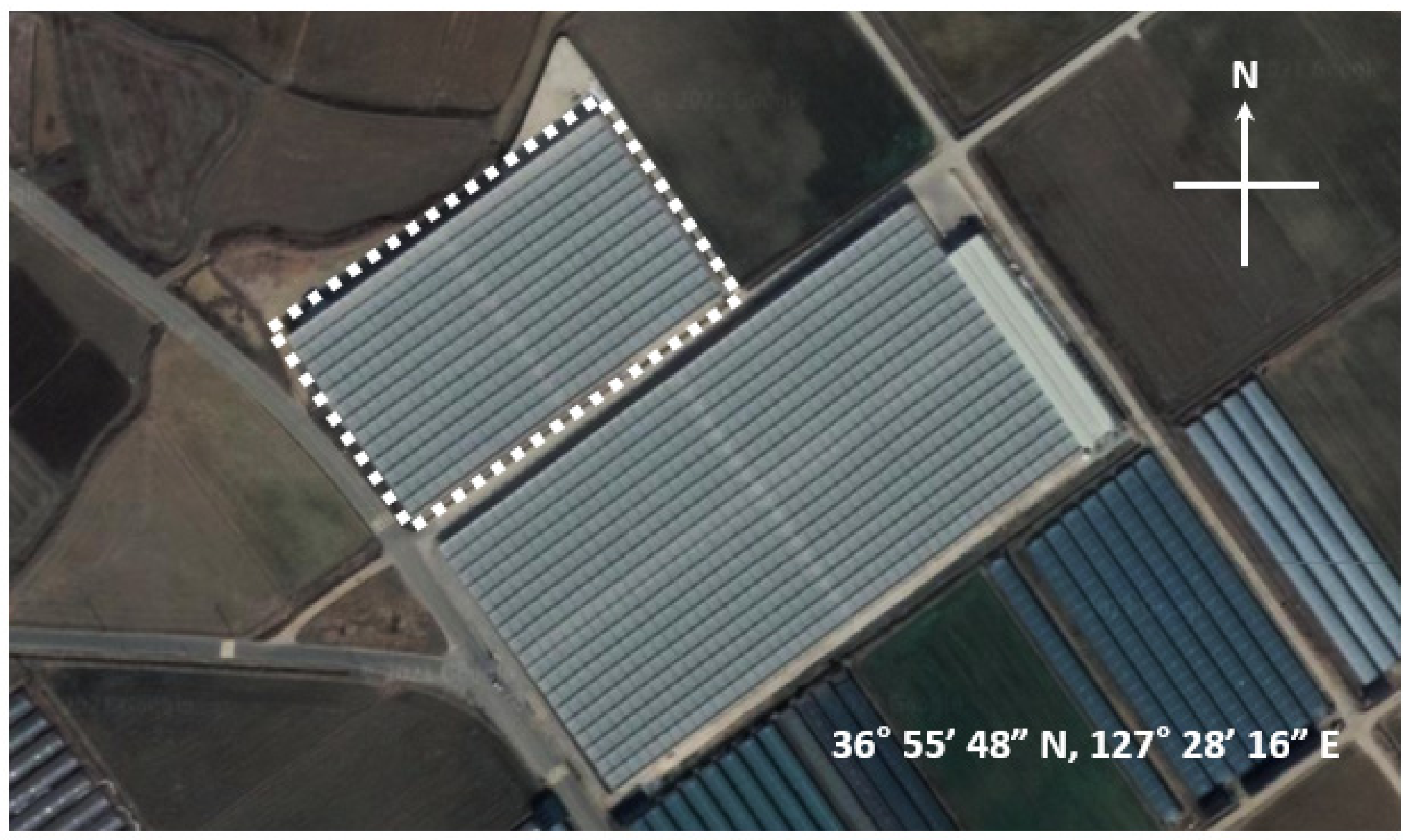
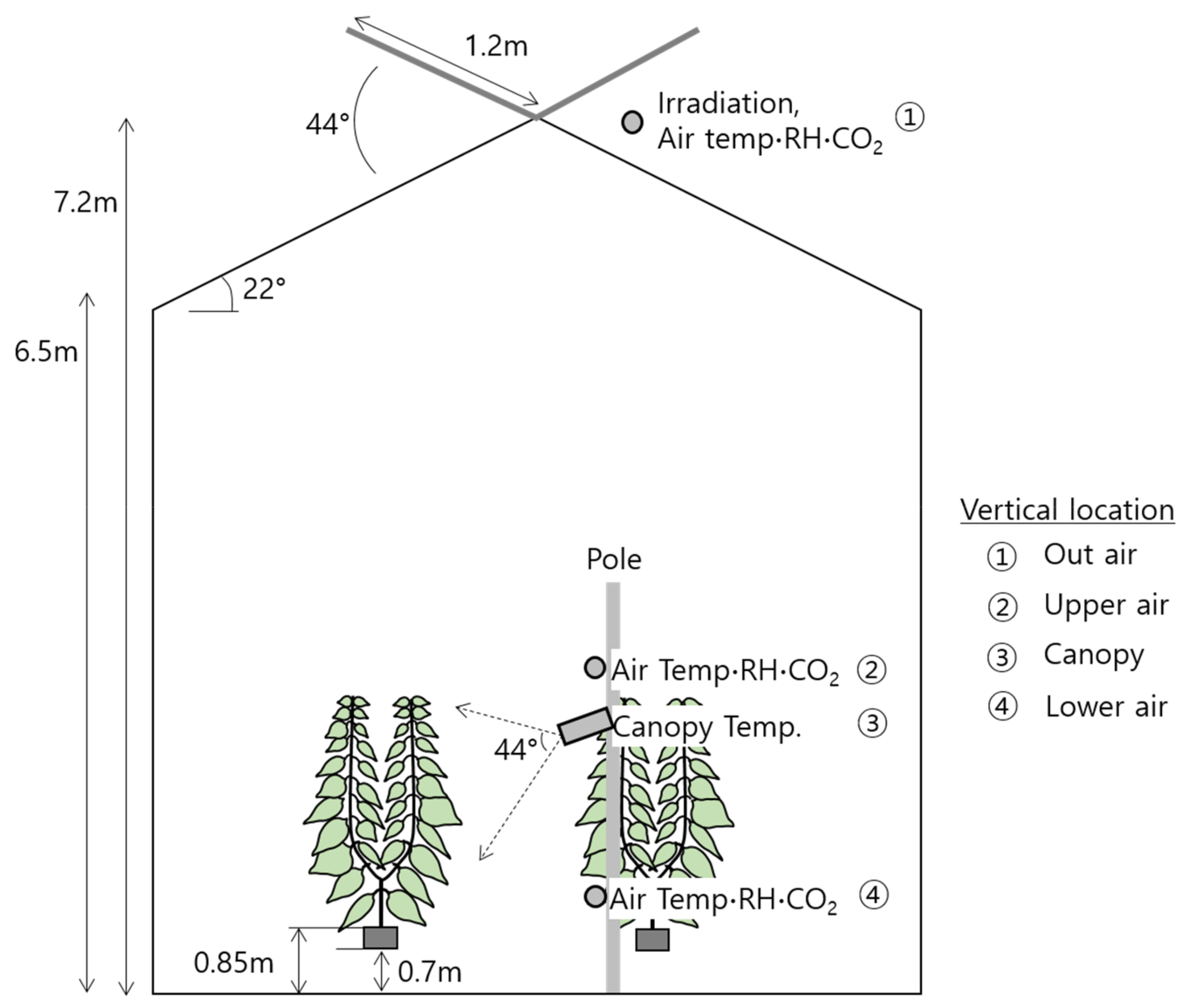
2.1. Target Greenhouse

The study target crop, bell pepper (Volante, Enza Zaden, Haling 1-E, 1602 DB Enkhuizen, the Netherlands), belongs to the family Solanaceae and is a species of the genus Capsicum. It was planted in a rock wool substrate on 6 July 2021. The plant density was 8.26 plant m⁻², the LAI at the crop growth stage of the study period was approximately measured to be 2.5, and the research period extended from 7 September to 6 October. The glass greenhouse was located in Jincheon, in a central province of South Korea (Figure 1). A schematic representation is shown in Figure 2. The roof covering material was 4 mm low iron glass, the outer wall was 16 mm polycarbonate, and no artificial light was installed.

2.2. Heterogeneously Scaled Models of Plant

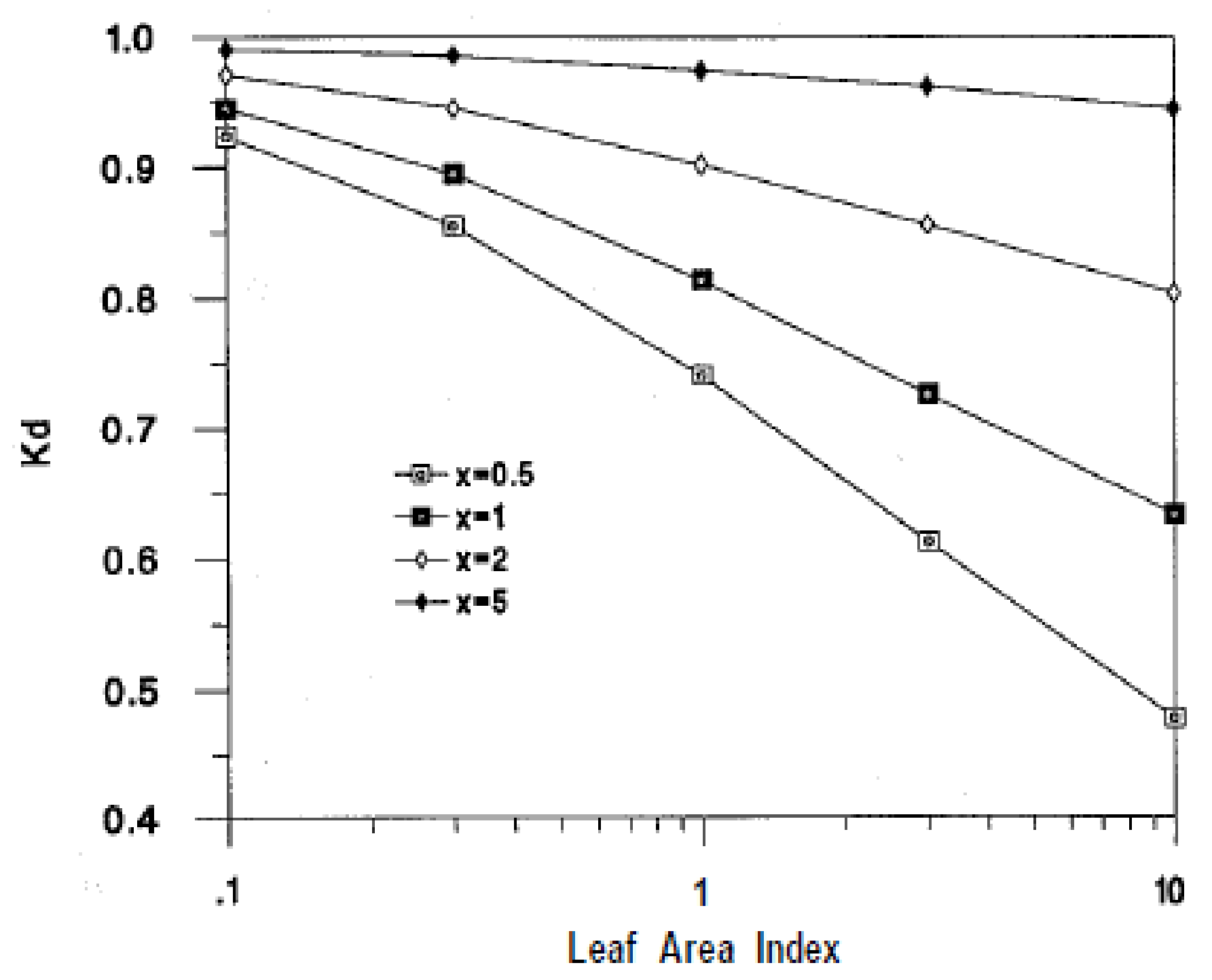
2.2.1. Extinction Coefficient

Campbell and Norman [20] presented physical quantities of the environmental climate and plants. To calculate solar energy, the direct beam, diffuse irradiation, and albedo must be estimated, as is expressed in Equations (1)–(3), respectively. The effect of albedo on the canopy can be negligible if the light absorptivity of the canopy is close to 1, the reflectivity by the canopy is insignificant, and the shortwave reflectivity of the fabric installed on the greenhouse soil is negligible.

$$S_b=S_{po}{\tau }^{m }$$

(1)

$$m=\frac{P_a}{101.3cos\Psi }$$

(2)

$$S_d=0.3\left(1-{\tau }^m\right)S_{po}cos\Psi$$

(3)

where $S_b$ is the flux density (W m⁻²) of beam radiation, $S_{po}$ is the extraterrestrial radiation, $S_d$ is the flux density of the scattered diffuse radiation, $\tau$ is the atmospheric transmittance, m is the airmass number, $P_a$ is the atmospheric pressure, and $\Psi$ is the zenith angle.

The average irradiance in the LAI tends to attenuate exponentially with the depth of the LAI. The beam, scattered diffuse, and scattered beam of solar irradiation will have different attenuation properties depending on the LAI depth. Assuming the canopy is a uniform horizontal absorber, the average irradiation can be predicted by the Lambert–Beer law. When generalizing the area distribution of the prolate or oblate spheroid of leaves, the extinction coefficient is expressed in Equation (4) according to the leaf angle distribution. The extinction characteristic of beam irradiation ($K_b$) can vary depending on the leaf angle distribution ($\chi$), which is the value obtained by dividing the leaf area projected on the horizontal plane by the leaf area projected on the vertical plane. If a leaf angle distribution is spherical, $\chi$ is close to 1; if there is a vertical distribution, $\chi$ is 0; if there is a horizontal leaf canopy, $\chi$ approaches infinity. The $\chi$ value for the wheat crop was reported to be 0.96 [20].

$$K_b=\frac{\sqrt{{\chi }^2+ta{n}^2\Psi }}{\chi +1.774{\left(\chi +1.182\right)}^{-0.773}}$$

(4)

The extinction coefficient of scattered diffuse irradiation ($K_d$) can be described as a function of the LAI and $\mathsf{\chi }$. It is reported that the functional relationship has similar characteristics to those shown in Figure 3.

As shown in Figure 1, the regression equation of $K_d$ for the case where $\mathsf{\chi }$ is 1 can be expressed as in Equation (5) for LAI (L), and the extinction coefficient ($K_{sb}$) for the scattered beam is the same as in Equation (6) [21].

$$K_d=f\left\{L, \mathsf{\chi }\right\}=0.0004L^4-0.0016L^3+0.0216L^2-0.1311L+{\left.0.9754\right|}_{\chi =1}$$

(5)

$$K_{sb}=\frac{0.46}{cos\left(\Psi \right)}$$

(6)

Evaluating $K_d$ based on Figure 3, we used a polynomial regression to enhance the accuracy. Fruit cluster leaf foliation in greenhouses in South Korea is usually carried out before the LAI exceeds 4, and this study corresponds to the case of LAI 2.5. When evaluating the regression model at LAI 4 or less, the RMSE (root mean square error), CV(RMSE) (coefficient of variation of RMSE), and R-squared were 0.0252, 0.0319, and 0.9804, respectively.

2.2.2. Boundary Layer Conductance

The boundary layer conductance of vapor ($g_{Va}$) and heat ($g_{Ha}$) (mol m⁻² s⁻¹) are affected by the wind speed ($u\left(z\right)$) for a molar density (ρ). Wind speed is not affected by the canopy structure as it rises to the height of the canopy in the vertical z direction. The wind speed is reduced as drag force is generated in the downward direction because of the hairs on the leaf surface or the air resistance component of the canopy. Given the vertical wind profile in a logarithm, the height at the canopy depth at which the wind speed is zero is called the roughness length. For rough surfaces such as tall crops and forest, the ground surface is not an appropriate reference level to express the height in the equilibrium boundary layer. The reference level is then displaced upwards by an amount that is called the zero plane displacement [22,23]. Roughness lengths for momentum ($z_M$) and heat ($z_H$), and the zero plane displacement ($d$), are important parameters for estimating the energy exchange between the ground and air [24]. The $g_{Va}$ (mol m⁻² s⁻¹) is expressed as in Equation (7). It was reported that the diabatic corrections for momentum (${\Psi }_M$) and heat (${\Psi }_H$) are not important under the condition of a wind speed of 3–4 m s⁻¹, and the values of $d$ = 0.65 h, $z_M$= 0.1 h, and $z_H$= 0.2$z_M$ can be estimated, where h is the height of the canopy [20].

$$g_{Va}=g_{Ha}=\frac{{0.4}^2\rho ·u\left(z\right)}{\left[\ln \left(\frac{z-d}{z_M}\right)+{\Psi }_M\right]\left[\ln \left(\frac{z-d}{z_H}\right)+{\Psi }_H\right]}$$

(7)

The stomatal conductance of vapor in the leaf ($g_{vs}$) is connected in series to the boundary layer conductance of vapor ($g_{va}$) (mol m⁻² s⁻¹). Vapor diffusing from the inside to the outside of the abaxial and adaxial leaf surfaces can be solved as parallel conductivity, which increases the overall conductivity. Equation (8) shows the conductance of vapor ($g_v$) on both sides [25].

$$g_v=\frac{g_{vs}^{ab}{g}_{va}}{g_{vs}^{ad}+g_{va}}+\frac{g_{vs}^{ad}{g}_{va}}{g_{vs}^{ad}+g_{va}}$$

(8)

where $g_{vs}^{ab}$ and $g_{vs}^{ad}$ are the abaxial and adaxial stomatal conductance of vapor, respectively.

2.2.3. Wind Speed

In the canopy structure, the wind speed of the boundary layer of the canopy from zero plane displacement is described by Equation (9). The wind speed inside the canopy has different characteristics from that outside the canopy. The u(z) inside the canopy is modeled using Equation (10) [26,27].

$$u\left(z\right)=\frac{u^{*}}{0.4}\ln \left(\frac{ z-d }{z_m}\right)$$

(9)

$$u\left(z\right)=u\left(h\right)·exp\left[a\left(\frac{z}{h}-1\right)\right]$$

(10)

where $u^{*}$ is the friction speed of wind and h is the canopy height. The friction speed is related to the magnitude of eddies, and it can be obtained by calculating other variables except for it [22].

The attenuation coefficient of the plant (a) is given by Equations (11) and (12) using the properties of the plant. The attenuation coefficient varies depending on the crop characteristics, which differ, for instance, for grass, maize, and coniferous forest, and can be obtained as follows [28].

$$a={\left(\frac{0.2L·h}{l_m}\right)}^{\frac{1}{2}}$$

(11)

$$l_m={\left(\frac{4wh}{\pi ·L}\right)}^{\frac{1}{2}}$$

(12)

where $l_m$ is the mean distance between leaves in the canopy and w is the leaf width.

2.2.4. Irradiation

The total irradiation ($I_c$) absorbed by the canopy can be interpreted as the sum of the irradiation of sunlit ($I_{sun}$) and shaded ($I_{sh}$) parts, which have the unit of W m⁻².

$$I_c=I_{sun}+I_{sh}$$

(13)

Ref. [21] indicated the beam, scattered diffuse, and scattered beam components for sunlit and shaded conditions. In this study, the irradiation could be calculated separately depending on whether sunlit or shaded for each LAI depth from Equations (14)–(20). Irradiation on sunlit parts can be divided into beam, scattered diffuse, and scattered beam, and the corresponding fraction can be applied.

The beam irradiation of sunlit parts ($I_{sun.S_b}$) (W m⁻²) is calculated based on the application of a fraction that attenuates according to the depth of LAI.

$$I_{sun.S_b}=S_b{f}_b\left(\Psi \right)=S_b({\alpha }_{lf}{K}_b{e}^{-K_b·L})$$

(14)

where $f_b$ is the beam fraction and ${\alpha }_{lf}$ is the absorptivity of the leaf for the beam.

Scattered diffuse irradiation of sunlit parts ($I_{sun.S_d}$) can be classified into upstream and downstream fluxes of diffuse beam irradiation [29]. $I_{sun.S_d}$ is described by Equation (15).

$$I_{sun.S_d}=S_d{f}_d\left(\Psi \right)=S_d\left\{{\alpha }_d{K}_d{e}^{-(K_d+K_b)·L}\right\}$$

(15)

where $f_d$ is the scattered diffuse fraction and ${\alpha }_d$ is the absorptivity of the scattered diffuse fraction.

Scattered beam irradiation of sunlit parts ($I_{sun.S_{sb}}$) includes a downward scattered beam and an upward beam component. In the canopy, the scattered beam and beam irradiation from beam radiation ($S_b$) are attenuated by $K_{sb}$. Since $I_{sun.S_{sb}}$ originates from $S_b$, a component excluding the up- and downstream of the beam can be expressed as in Equation (16).

$$I_{sun.S_{sb}}=S_b{f}_{sb}\left(\Psi \right)=S_b\{{\alpha }_{sb}{K}_{sb}{e}^{-(K_{sb}+K_b)·L}-{\alpha }_{lf}{K}_b{e}^{-2K_b·L}\}$$

(16)

where $f_{sb}$ is the scattered beam fraction and ${\alpha }_{sb}$ is the absorptivity of the scattered beam.

Simultaneously, total irradiations of the scattered diffuse ($I_{c.S_d}$) and scattered beam ($I_{c.S_{sb}}$) are given by Equations (17) and (18), respectively.

$$I_{c.S_d}=S_d({\alpha }_d{K}_d{e}^{-K_d·L})$$

(17)

$$I_{c.S_{sb}}=S_b({\alpha }_{sb}{K}_{sb}{e}^{-K_{sb}·L}-{\alpha }_{lf}{K}_b{e}^{-K_b·L})$$

(18)

where ${\alpha }_{sb}$ is the absorptivity of the scattered beam.

Irradiation of shade is classified into the scattered diffuse and scattered beam components, and the corresponding fraction can be applied. The shade fraction is obtained by subtracting the sunlit fraction from the total irradiation. Scattered diffuse irradiation ($I_{sh.S_d}$) and scattered beam irradiation ($I_{sh.S_{sb}}$) of shade can be expanded as Equations (19) and (20), respectively.

$$I_{sh.S_d}=I_{c.S_d}-I_{sun.S_{sd}}=S_d\left\{{\alpha }_d{K}_d{e}^{-K_d·L}-{\alpha }_d{K}_d{e}^{-(K_d+K_b)·L}\right\}$$

(19)

$$\begin{gathered} I_{sh.S_{sb}}=I_{c.S_{sb}}-I_{sun.S_{sb}}=S_b\left[{\alpha }_{sb}\left\{K_{sb}{e}^{-K_{sb}·L}-K_{sb}{e}^{-(K_{sb}+K_b)·L}\right\}- \\ {\alpha }_{lf}\left\{K_b{e}^{-K_b·L}-K_b{e}^{-2K_b·L}\right\}\right] \end{gathered}$$

(20)

To obtain the intercepted irradiation for each LAI, it is necessary to integrate based on the LAI interval of the canopy ($L_c$), where the fraction intercepted by the canopy can be expressed by the 1-transmissivity, and the non-intercepted irradiation can be developed as the penetrated fraction (

Table 1. Equations of intercepted and penetrated irradiation of sunlit and shaded areas in the canopy for beam, scattered diffuse, and scattered beam irradiation.

		Intercept		Penetrate
Sunlit	Beam	$S_b{\alpha }_{lf}(1-e^{-K_b·L_c})$	(21)	$S_b{\alpha }_{lf}{K}_b(e^{-K_b·L_c})$	(26)
	Scattered diffuse	$S_d{\alpha }_d{K}_d\left[\frac{\left\{1-e^{-(K_d+K_b)·L_c}\right\}}{K_d+K_b}\right]$	(22)	$S_d{\alpha }_d{K}_d\left[\frac{\left\{e^{-(K_d+K_b)·L_c}\right\}}{K_d+K_b}\right]$	(27)
	Scattered beam	$S_b\left[\frac{{\alpha }_{sb}{K}_{sb}\left\{1-e^{-(K_{sb}+K_b)·L_c}\right\}}{K_{sb}+K_b}-\frac{{\alpha }_{lf}\left(1-e^{-2K_b·L_c}\right)}{2}\right]$	(23)	$S_b\left[\frac{{\alpha }_{sb}{K}_{sb}\left\{e^{-(K_{sb}+K_b)·L_c}\right\}}{K_{sb}+K_b}-\frac{{\alpha }_{lf}\left(e^{-2K_b·L_c}\right)}{2}\right]$	(28)
Shade	Scattered diffuse	$S_d{\alpha }_d\left[1-e^{-K_d·L_c}-\frac{K_d\left\{1-e^{-(K_d+K_b)·L_c}\right\}}{K_d+K_b}\right]$	(24)	$S_d{\alpha }_d\left[e^{-K_d·L_c}-\frac{K_d\left\{e^{-(K_d+K_b)·L_c}\right\}}{K_d+K_b}\right]$	(29)
	Scattered beam	$S_b\left[{\alpha }_{sb}\left[1-e^{-K_{sb}·L_c}-\frac{\left\{1-e^{-(K_{sb}+K_b)·L_c}\right\}{K}_{sb}}{K_{sb}+K_b}\right]-{\alpha }_{lf}\left[1-e^{-K_b·L}-\frac{\left\{1-e^{-2K_b·L_c}\right\}}{2}\right]\right]$	(25)	$S_b\left[{\alpha }_{sb}\left[e^{-K_{sb}·L_c}-\frac{\left\{e^{-(K_{sb}+K_b)·L_c}\right\}{K}_{sb}}{K_{sb}+K_b}\right]-{\alpha }_{lf}\left[e^{-K_b·L}-\frac{\left\{e^{-2K_b·L_c}\right\}}{2}\right]\right]$	(30)

).

To estimate the photosynthetic efficiency, the net assimilation of the canopy should be analyzed by distinguishing the sunlit and shaded areas for the intercepted irradiation. The penetrated irradiation on the soil can be regarded as a wasted light resource in the limited greenhouse volume, and to predict the absorptivity of the beam according to the leaf angle distribution and zenith angle, it will be necessary to estimate the amount of beam compared to the diffuse and scattered beam from the total irradiation. In contrast, the big leaf model cannot explain the effect of LAI based on the light environment of the shoot apical meristem, fruit set, and skin color development of the fruit.

2.3. Theoretical Mechanism

2.3.1. Transpiration and Canopy Temperature

In a previous study, it was suggested that the leaf reflectivity for direct irradiation is 0.15, the canopy reflectivity for scattered diffuse irradiation is 0.036, the canopy reflectivity for the scattered beam is 0.04, and the leaf absorptivity for the beam is 0.85 [21]. Furthermore, it was also reported that the canopy absorptivity for the scattered diffuse is 0.95 or more, the deciduous forest reflectivity is 0.1–0.2, and the leaf emissivity is 0.95 [20].

The apparent psychrometer constant (${{\rm Y}}^{*}$) is defined as the sum of the boundary layer and radiative conductance ($g_{Hr}$) and the ratio of conductance of vapor ($g_v$) for the thermodynamic psychrometer constant (${\rm Y}$). In the canopy environment, when estimating conductance, it was revealed that excluding radiative conductance is more accurate as a rule of thumb, and $g_{Ha}$ was considered equal to $g_{Va}$[9,30].

$${{\rm Y}}^{*}={\rm Y}\frac{g_{Hr}}{g_v}=\frac{c_p}{\lambda }\frac{g_{Ha}}{g_v}$$

(31)

where $c_p$ (J mol⁻¹ °C⁻¹) is the specific heat of the air and $\lambda$ (J mol⁻¹) is the latent heat of vaporization.

Absorbed radiation for short- and longwaves can be classified into beam, diffuse, and scattered beam components, and canopy evaporative water loss ($E_{cpy}$) specifies the integration of the LAI, so that the amount of transpiration for multi-layers can be developed as per Equation (32).

$$\begin{gathered} \lambda E_{cpy}=\frac{s\left(R_{abs}-L_{oe}\right)+{{\rm Y}}^{*}\lambda g_v\left(\frac{D}{P_a}\right)}{s+{{\rm Y}}^{* }} \\ =\frac{s}{s+{{\rm Y}}^{*}}\left(\begin{array}{c}{\tau }_{cv.b}{\tau }_{sc.b}{F}_b{S}_b{\alpha }_{lf}\left(1-e^{-K_b·L_c}\right)\\ + {\tau }_{cv.d}{\tau }_{sc.d}{F}_d{S}_d\left[\frac{{\alpha }_d\left\{1-e^{-(K_d+K_b)·L_c}\right\}{K}_d}{K_d+K_b}\right]\\ + {\tau }_{cv.b}{\tau }_{sc.b}{F}_b{S}_b\left[\frac{{\alpha }_{sb}\left\{1-e^{-(K_{sb}+K_b)·L_c}\right\}{K}_{sb}}{K_{sb}+K_b}-\frac{{\alpha }_{lf}\left(1-e^{-2K_b·L_c}\right)}{2}\right]\\ +{\tau }_{cv.d}{\tau }_{sc.d}{F}_d{S}_d{\alpha }_d\left[1-e^{-K_d·L_c}-\frac{\left\{1-e^{-(K_d+K_b)·L_c}\right\}{K}_d}{K_d+K_b}\right]\\ +{\tau }_{cv.b}{\tau }_{sc.b}{F}_b{S}_b\left[\begin{array}{c}{\alpha }_{sb}\left[1-e^{-K_{bs}·L_c}-\frac{\left\{1-e^{-(K_{sb}+K_b)·L_c}\right\}{K}_{sb}}{K_{bs}+K_b}\right]\\ -{\alpha }_{lf}\left[1-e^{-K_b·L_c}-\frac{\left\{1-e^{-2K_b·L_c}\right\}}{2}\right]\end{array}\right]\\ +F_a{\alpha }_l{L}_a{L}_c-F_e{L}_{oe}{L}_c\end{array}\right) \\ +\frac{{{\rm Y}}^{*}}{s+{{\rm Y}}^{* }}\lambda g_v\left(\frac{D}{P_a}\right) \end{gathered}$$

(32)

where $s$ is the slope of the saturation mole fraction in °C⁻¹. $R_{abs}$, $L_{oe}$, $L_a$, $S_{sun}$, and $S_{sh}$ are the absorbed short- and longwave irradiation, out-emitted longwave radiation, atmospheric longwave radiation, shortwave for the sunlit fraction of the canopy, and shortwave for the shaded fraction of the canopy, respectively, which have the units of W m⁻², while $D$ is the vapor of the deficit in kPa. ${\tau }_{cv.b}$, ${\tau }_{cv.d}$, ${\tau }_{sc.b}$, and ${\tau }_{sc.d}$ are the transmissivity of the beam for the covering material, diffuse for the covering material, beam for the screen curtain, and diffuse for the screen curtain, respectively. $F_b$, $F_d$, $F_a$, and $F_e$ are the view factors of beam radiation, diffuse radiation, air, and the environment, respectively. $L_a$ and $L_{oe}$ are the air fraction of the longwave and the out-emitted longwave fraction, respectively.

To obtain the canopy temperature, Equation (32) can be substituted for Equation (33) with some modifications assuming that the numbers of incoming and outemitted longwaves on the canopy are the same.

$$T_{cpy}=T_a+\frac{{{\rm Y}}^{*}}{s+{{\rm Y}}^{*}}\left(\begin{array}{c}\frac{\left(\begin{array}{c}{\tau }_{cv.b}{\tau }_{sc.b}{F}_b{{\displaystyle \int }}_0^{L_c}{S}_b{f}_b\left(\Psi \right) dL\\ +{\tau }_{cv.d}{\tau }_{sc.d}{F}_d{{\displaystyle \int }}_0^{L_c}{S}_d{f}_d\left(\Psi \right) dL\\ +{\tau }_{cv.b}{\tau }_{sc.b}{F}_b{{\displaystyle \int }}_0^{L_c}{S}_{sb}{f}_{sb}\left(\Psi \right)dL\\ +{\tau }_{cv.d}{\tau }_{sc.d}{F}_d{{\displaystyle \int }}_0^{L_c}{S}_d\left\{1-f_d\left(\Psi \right)\right\}dL\\ +{\tau }_{cv.b}{\tau }_{sc.b}{F}_b{{\displaystyle \int }}_0^{L_c}{S}_b\left\{1-f_{sb}\left(\Psi \right) \right\}dL\end{array}\right)}{c_p{g}_{Hr}}\\ -\frac{D}{{{\rm Y}}^{*}{P}_a}\end{array}\right)$$

(33)

The view factor is the ratio of the light radiated by one object to that received by another. For the view factor of the canopy, $F_b$= cos$\Psi$ and $F_d$=$F_a$=$F_e$= 1 were estimated. Considering the view factors of the upper and lower hemisphere longwaves for the sky and ground, it can be estimated that $F_{a }$=$F_e$= 0.5. The view factor for the beam component already includes the zenith angle when calculating the air mass, and hence the view factor of the beam component can be excluded when calculating the canopy temperature.

The light compensation point of bell pepper was reported to be 21.83 ± 0.58 μmol m⁻² s⁻¹ [31]. Unlike an open-field culture, the target greenhouse was made of polycarbonate material with a side wall height of 6.5 m for insulation from the external environment. Under environmental conditions where there were various steel structures and strings inside the greenhouse, and the plant height was nearly 2.5 m, when the zenith angle exceeded 74°, the shortwave was measured to be approximately 10 W m⁻² s⁻¹. It was thus considered to have dropped below the light compensation point. Based on Equations (32) and (33), transpiration and the canopy temperature can be simply developed as follows when the zenith angle exceeds 74°.

$$E=\frac{{{\rm Y}}^{*}{g}_v\left(\frac{D}{P_a}\right)}{s+{{\rm Y}}^{* }}$$

(34)

$$T_{cpy}=T_a-\frac{D}{P_a\left(s+{{\rm Y}}^{*}\right)}$$

(35)

2.3.2. Energy Flux between the Canopy and Air

The Penman–Monteith model, which is the basis for this research model, satisfies the isothermal condition by approximating the ratio of the canopy to the air temperature using Penman linearization, and the absorbed energy is described by the following balance equation.

$$R_{abs}=L_{oe}+H+\lambda E$$

(36)

where sensible heat exchange ($H$) is given by Equation (37).

$$H=c_p{g}_{Ha}\left(T_{cpy}-T_a\right)$$

(37)

Fitter and Hay [32] expressed a non-isothermal condition in which the temperature is changed.

If

$$R_{abs}<L_{oe}+H+\lambda E$$

(38)

then the canopy temperature will be cooled, whereas if

$$R_{abs}>L_{oe}+H+\lambda E$$

(39)

then the canopy temperature will rise.

The air temperature was substituted for the longwave absorbed by the canopy under the isothermal condition (Equations (40) and (41)), but the longwave was replaced by the canopy temperature under the non-isothermal condition (Equation (42)).

$$R_{abs}=S_{sun}+S_{sh}+L_a$$

(40)

$$L_a={\epsilon }_a\sigma T_a^4$$

(41)

$$L_{cpy}={\epsilon }_{cpy}\sigma T_{cpy}^4$$

(42)

where $\sigma$ is the Stefan–Boltzmann constant, ${\epsilon }_a$ and ${\epsilon }_{cpy}$ are the emissivity of air and the canopy, respectively, and $L_{cpy}$ is the longwave from the canopy in W m⁻².

Consequently, the heat flux between the air and the canopy can be obtained by the difference calculated from Equations (36)–(42).

2.3.3. Stomatal Conductance

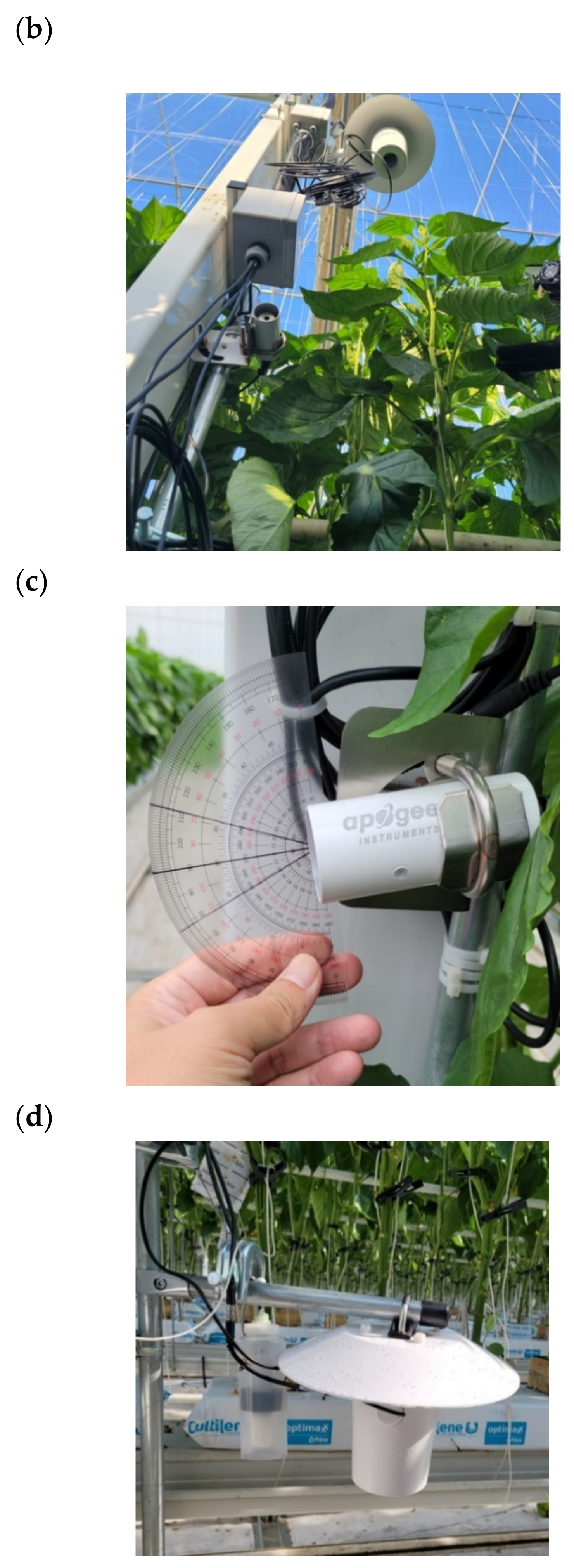
The stomata close when the CO₂ concentration is high and they open when the humidity is low. Evidently, the photosynthetic efficiency can be used as a proportional coefficient, and there is a basic stomatal conductivity by respiration at night [33,34,35,36]. In this study, the stomatal conductivity was estimated to be 90 μmol m⁻² s⁻¹ [37,38,39]. However, generally, the conductance in sunlit parts is larger than in the shade [40,41], but the differences may not be discernible in a moderately shaded environment [42].

To establish the stomatal conductance model, the stomatal conductance was measured in the target greenhouse fertilized with CO₂ for 2 days under different weather conditions (Figure 4), with a porometer, by randomly selecting five individuals from 28,000 plants. The shortwave was measured inside the greenhouse.

To summarize the measurements, the stomatal conductance in sunlit parts was approximately 9% higher than that in the shade, and the conductance on the abaxial side was nearly 50% higher than that on the adaxial side. As described in Section 3.1.2, the overall LAI was measured to be 2.5. If the LAI is divided into three, LAI3 becomes 1.67–2.50, LAI2 0.84–1.67, and LAI1 0.00–1.66. Compared to the measurements at LAI3, the conductance at LAI2 was approximately 80% and that at LAI1 was 40%. In this study, the proportional equation was applied to the conductance of LAI2 and LAI1, and additional weighted values were not substituted in the sunlight and shade.

To obtain the modeled stomatal conductance of the abaxial side for LAI3, using the measured shortwave, CO₂ concentration, and relative humidity (RH) as independent variables, the nonlinear multiple regression was performed as follows (IBM SPSS Statistics, ver. 26, release 26.0.0.0)

$$g_{vs}^{ab}=-0.795-\left\{1-e^{-0.925{\left(\frac{Rad\ast RH}{C{O}_2}\right)}^2}\right\}+e^{0.774\left(\frac{Rad\ast RH}{C{O}_2}\right)}$$

(43)

where $RH$ is the relative humidity and $Rad$ is the irradiated shortwave above the canopy in W m⁻².

2.4. Measurements

An infrared sensor (SI-111-SS, Apogee, Logan, UT, USA) was installed to measure the canopy temperature for LAI2.5 and plant height of 2.5 m. The viewing angle was adjusted by tilting it downward to 44° from the two training stems to the height of the plant. The period during which this study was conducted was growth stage 1, and the height of the crop was 2.5 m. The height of the crop that could be measured from the viewing angle of the infrared sensor was 2.5 m. It was necessary to measure the whole LAIs of the crop canopy in our work. An aspirated radiation shield (TS-100, Apogee, Logan, UT, USA) was applied to the temperature and humidity sensor (ATMOS-14, Meter, Pullman, WA, USA) to measure the air climate for the lower and upper parts of the canopy. The different mechanical sizes from each manufacturer of the sensor and shield were solved through a customized adapter. To measure the external weather, a pyranometer (SP-510-SS, Apogee, Logan, UT, USA) and a temperature-humidity sensor with the same aspirated radiation shield as the inside were installed. All measurements were collected in a data logger (CR1000X, Campbell scientific, Logan, UT, USA), and were stored in the Kangwon National University Biosystems Lab server through LTE communication. Sensors were installed next to the cube on the substrate, the body of the plant, and the shoot apical meristem in the vertical position, and set up in the center and at each corner in a horizontal location.

The LAI and stomatal conductivity were measured with a portable ceptometer (LP-80, Meter, USA) and porometer (SC-1, Meter, Pullman, WA, USA). The irradiation in the canopies was measured with a portable pyranometer (SR05 & LI-19, Hukseflux, Delft, South Holland, the Netherlands). The wind speed was measured through an anemometer (TES1340, TES, Neihu Dist., Taipei, Taiwan).

The positions and specifications of the sensors as shown in Figure 5, Figure 6 and Figure 7 and

Table 2. Specification of sensors used in this study.

Sensor	Picture	Measurement	Accuracy	Operating Temperature	Model Name	Manufacturer
Pyranometer		Spectral range: 285~3000 nm	±5%	-40~80 °C	SR05	Hukseflux
				-10~40 °C	LI-19
		Spectral range: 385~2105 nm	±5%	-50~80 °C	SP-510-SS	Apogee
Thermometer, hygrometer		Air temperature	±0.2%	-40~80 °C	ATMOS 14	Meter
		Air humidity	±2%	0~80 °C, 100% RH
		Aspirated radiation shield	-	-40~70 °C	TS-100	Apogee
Infrared sensor		Canopy temperature, spectral range: 8~14 μm	0.2 °C at -30~65 °C	-50~80 °C, 100% RH	SI-111-SS	Apogee
			0.5 °C at -40~80 °C
Porometer		Leaf conductance range: 0~1000 mmol m−2 s−1	±10% at 0~500 mmol	5~40 °C, 100% RH	SC-1	Meter
Ceptometer		Leaf area index, Spectral range: 400~700 nm	±5%	0~50 °C, 100% RH	LP-80	Meter
Anemometer		Wind velocity	±3%	0~50 °C	TES1340	TES
CO2		Carbon dioxide	±40 ppm	-40~60 °C	GMP-252	Vaisala
Data logger		Data logging	Processor: 32 bit, 100 MHz	-40~80 °C	CR1000X	Campbell scientific

. Figure 8 shows the sensors installed in the greenhouse.

In this study, the method devised to measure the LAI was to use the structure of the ceptometer and crop row. The probe length of the ceptometer was 80 cm, the distance from the center of the cube to the center of the aisle was 75 cm, and the ceptometer was tilted (Figure 9). For 20 random plants, the LAI measurements were multiplied by two because the bell pepper grew by way of two-stem V-type training method.

2.5. Parametrization

Environmental values referenced from the measurements and literature were substituted into model equations (

Table 3. Input variables to prove Equations (32) and (33).

Item	Symbol	Value	Unit	Remark
LAI	L	2.50	-	Measure
Wind speed a	u(z)	0.80	m s−1	Measure
Covering material Transmissivity b	τcv.b	0.90	-	Specification of manufacturer
	τcv.d	0.90	-
	τcv.bs	0.90	-
Canopy view factor	Fb	cosΨ	-	Campbell and Norman, 1998
	Fd	1.00	-
	Fbs	1.00	-
	Fa	0.50
	Fe	0.50	-
Radiation absorptivity	αlf	0.85	-	Pury and Farqhar, 1997
	αsb c	-	-
	αl	0.95	-	Campbell and Norman, 1998
	αd	0.95	-
Leaf angle distribution	χ	0.96	-
Canopy emissivity	εcpy	0.95	m
Plant height d	h	2.50	m	Measure
Leaf width	w	0.15	m	Measure
Air temperature	Ta	-	°C	Measure
Relative humidity	RH	-	%	Measure
Stomatal conductance	$g_{vs}^{ab}$	-	mol m−2 s−1	Measure
	$g_{vs}^{ad}$	-		Measure

^a Wind speed was measured in the boundary layer of the air just above the canopy in the greenhouse running an air circulation fan throughout the 24-h period. ^b In the manufacturer’s specification for the covering material, transmissivity was described as 0.9 without any distinction for beam, diffuse, and scatter irradiation. In this study, 0.9 was equally applied. ^c Absorptivity of the scattered beam is estimated to be ${\alpha }_{sb}=e^{\frac{-2·{\rho }_h·K_b}{1+K_b}}$. ^d Plant height is a measure of the height from the ground to the shoot apical meristem.

). As described in Equations (32) and (33), model equations were the final results that covered both the environmental climate and plants in the greenhouse.

As mentioned in Section 2.2.1, Equations (32) and (33) were mutually exchangeable. Equation (33) was compared to the canopy temperature measurements, and based on the results of the comparison, the irrigation volume (Equation (32)) could be revealed.

By substituting the calculated transpiration into Equations (36)–(39), the heat flux of the environmental plant was suggested.

3. Results

3.1. Actual Measurements

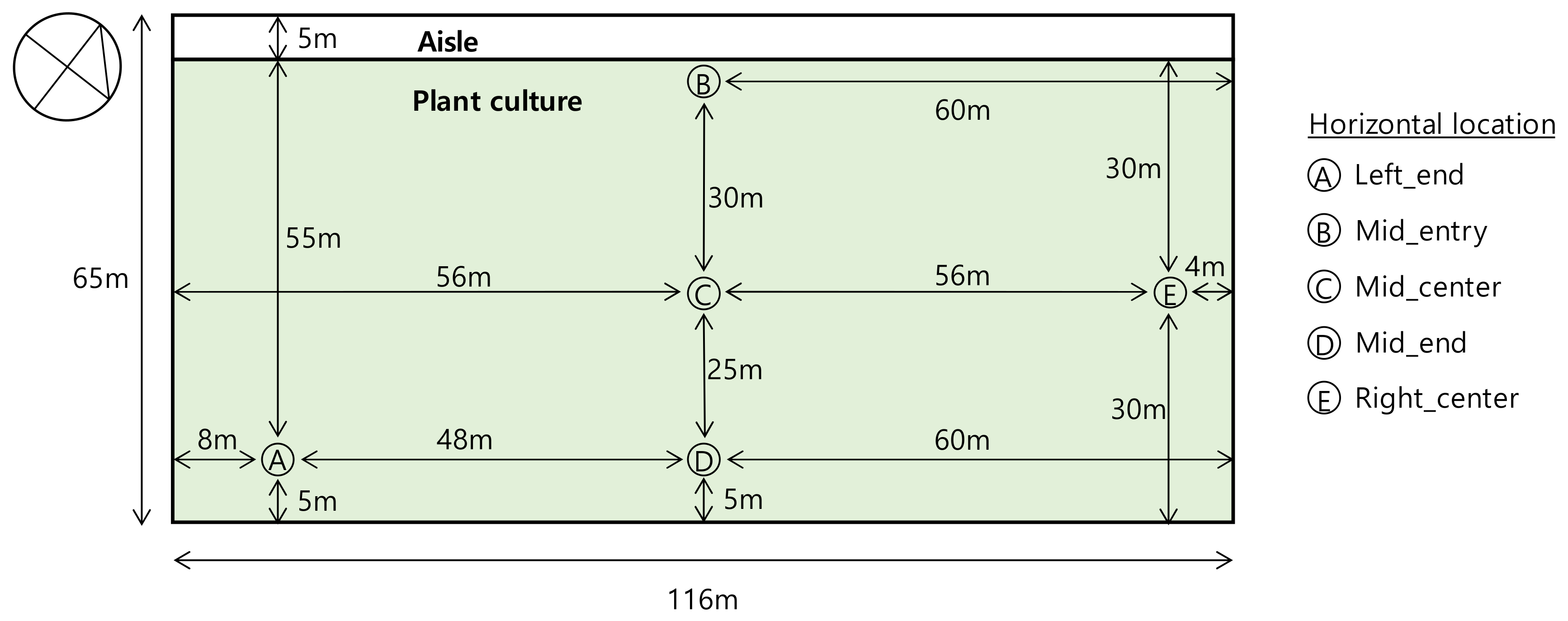
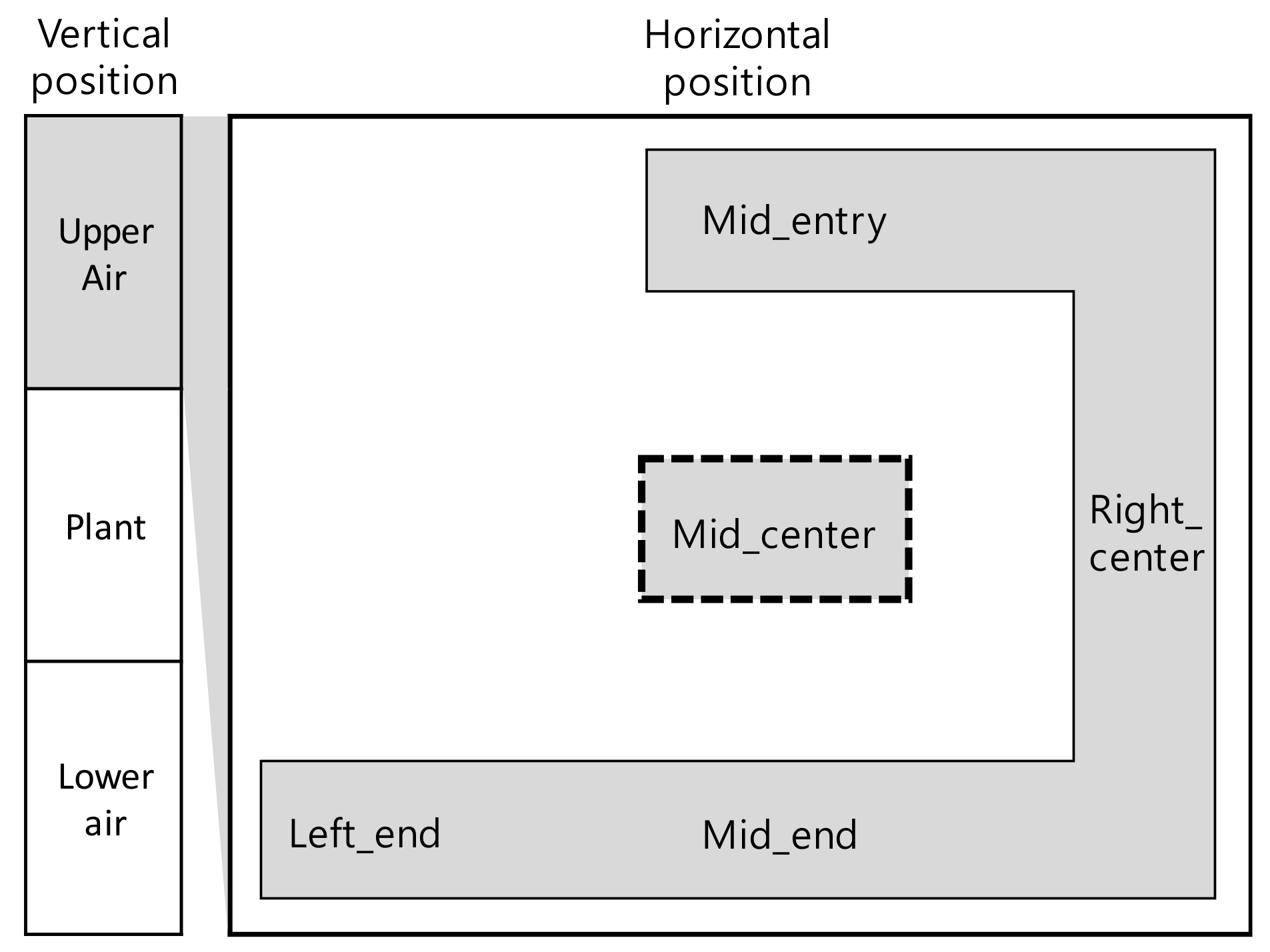
3.1.1. Measurements by Position

Generally, the climate measurement location referenced when controlling the greenhouse was referred to as the mid-center position. In this study, measurements from the mid-center sensor were selected as the temperature, humidity, and CO₂ values.

It was deduced that the deviation between the measured air and canopy temperatures from all five horizontal positions and those from the mid-center position was negligible. Humidity was considered to vary depending on the horizontal position, and when the humidity of the mid-center position was applied as a representative value, the average p-value was 0.004. CO₂ was artificially fertilized in the greenhouse, but tubes for CO₂ fertilization were not installed underneath all substrates; instead, they were installed underneath one substrate in two. Half of the CO₂ tubes were mounted in the mid-center area, and the other half were mounted in the remaining areas. Considering these circumstances of CO₂ fertilization, the p-value in this study was less than 0.01.

The error levels of the measurements between the whole and the mid-center positions in the greenhouse environment are summarized in

Table 4. Statistical significance test of sensor value at the mid-center position.

		Horizontal			Vertical
		5 Full a	Mid b	F c	Upper d	Lower e	F c
Ta	Upper air	22.8	22.6	1.0	22.6	22.7	1.1
	Lower air	22.9	22.8	1.0
RH	Upper air	86.4	88.3	1.2 ***	88.3	87.2	1.9 ***
	Lower air	86.3	87.2	1.1 **
CO2	Upper air	572.0	589.1	1.0 **	589.1	610.9	1.0 ***
	Lower air	583.6	610.9	1.0 **
Tcpy	Plant	22.8	22.5	1.0 **	-	-	-

Ta is the air temperature, Tcpy is the canopy temperature in °C, RH is the relative humidity in %, and CO₂ is the carbon dioxide concentration in ppm. The number of observations sampled is 720. ^a,b Measurements were collected hourly and each time, an average was taken from five full, mid-horizontal position measurements. ^c Based on the results of the F-test, the significance level was analyzed by equal or heterogeneous variances where ** p <0.01, *** p <0.001. ^d,e Measurements were collected hourly from vertical upper air and lower air positions.

.

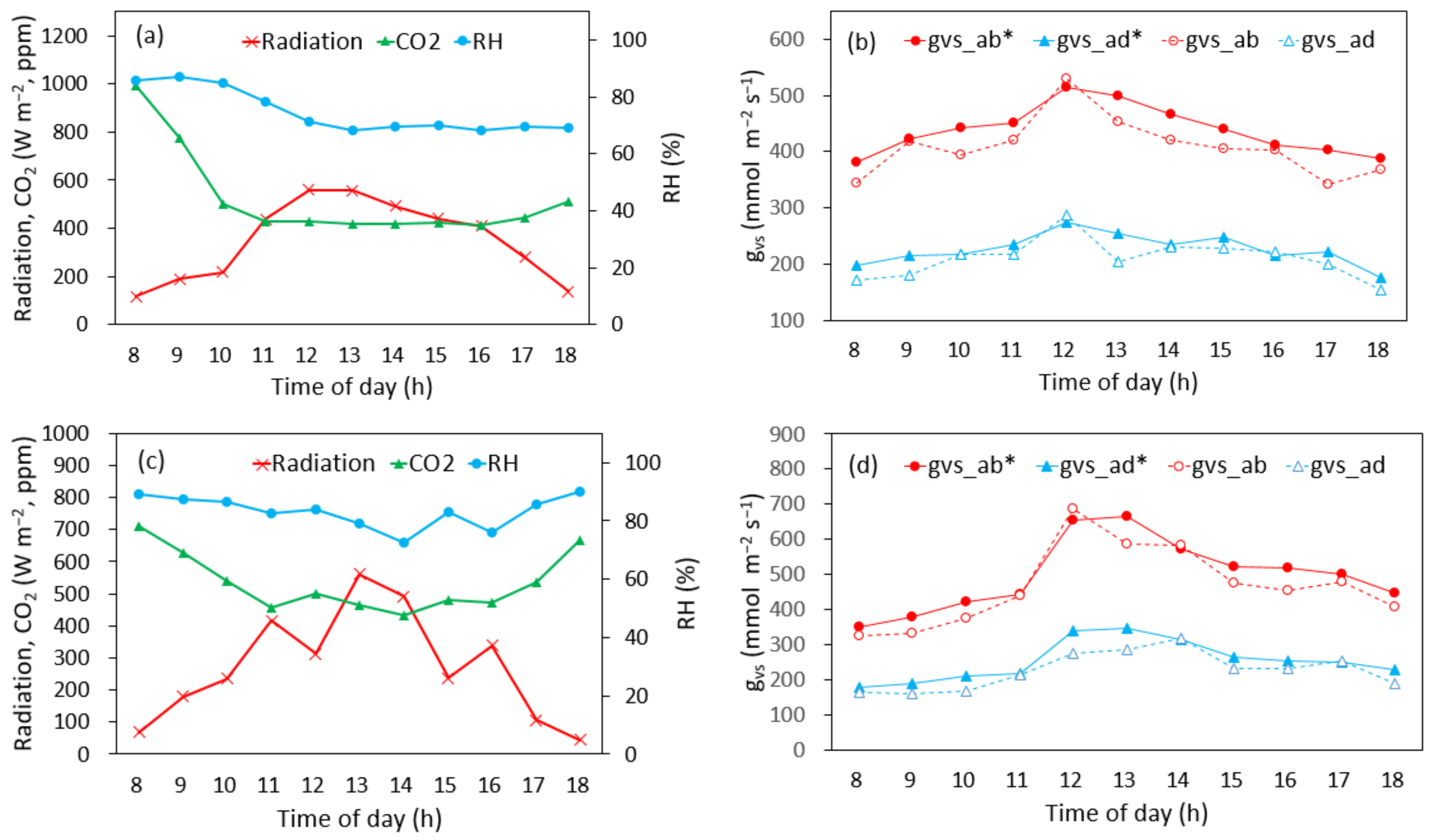
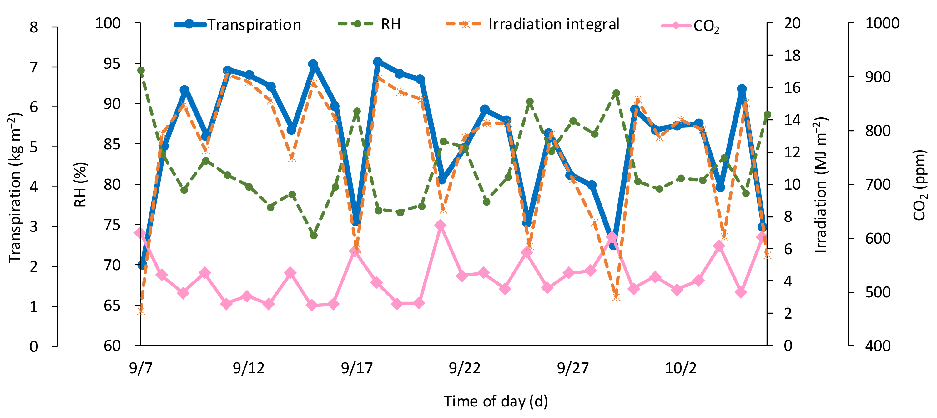
3.1.2. Other Measurements

During photosynthesis, the difference between the actual air and cooled canopy temperature was measured. The canopy temperature was lower than the air temperature due to a cooling effect only during the daytime. The measurement of stomatal conductance was already mentioned in the previous section, where the LAI was measured to be 2.5. During this study, the air circulation fan was operated over 24 h, the ventilators were opened by an average of 36% on the left and right sides, and the average wind speed of the outside air was approximately 1 m s⁻¹ (obtained from Korea Meteorological Administration data). The wind speed at 0.1 m above the canopy was measured (average of 0.8 m s⁻¹) with an anemometer. The wind speed for each LAI was calculated using Equations (9) and (10), and applied to Equations (32) and (33).

3.2. Model Calculation by LAI

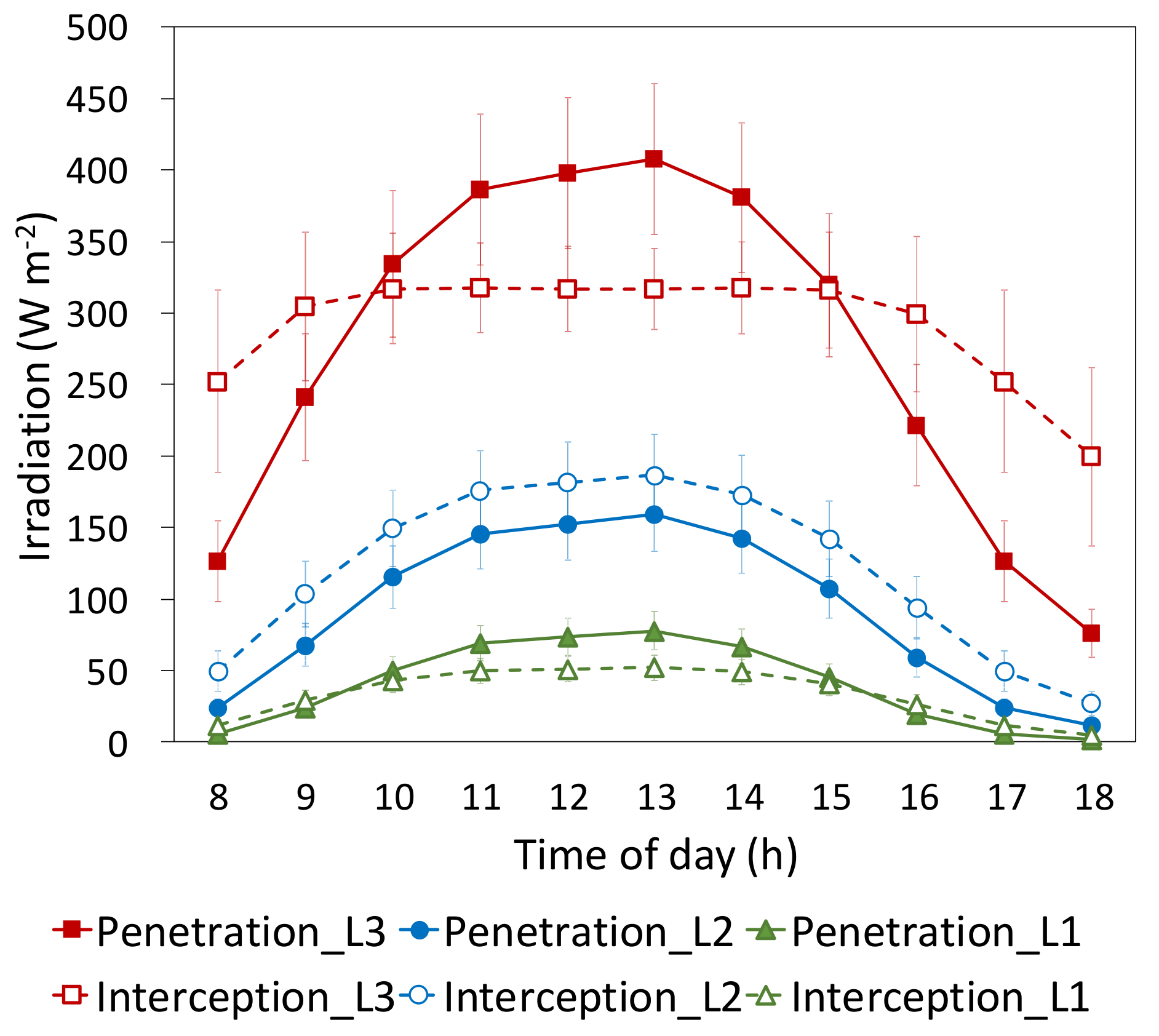
3.2.1. Irradiation

The beam, scattered diffuse, and scattered beam irradiation were calculated for sunlit areas. Irradiation of shaded areas, meanwhile, was calculated for the scattered diffuse and scattered beam (

Table 5. Statistical comparison of canopy temperatures from model and measurements.

R-Squared Score	Correlation Coefficient	RMSE	Residual Sum
0.979	0.989	0.457	−6.889 × 10−12 ***

p *** <0.001.

).

The calculations for sunlit and shaded areas revealed that direct beam irradiation played the biggest role compared to all other irradiations. For the sunlit and shaded intercept, the beam component in LAI3 occupied 74.7% of all irradiation components, 92.3% in LAI2, and 97.7% in LAI1.

Compared to the intercepted irradiation in sunlit areas, the average fractions in shaded areas were 8.4% in LAI3, 8.8% in LAI2, and 6% in LAI1. For the penetrated irradiation in sunlit areas, the fractions in shaded areas were 43.7% in LAI3, 23.5% in LAI2, and 11.4% in LAI1.

In sunlit areas, an intercepted irradiation in LAI3 was saturated from 9 a.m. to 4 p.m. and then decreased substantially in LAI1. In LAI2, the intercepted irradiation tended to be larger than that of the penetrated irradiation, and in LAI1, the penetrated irradiation was high at around noon (Figure 10).

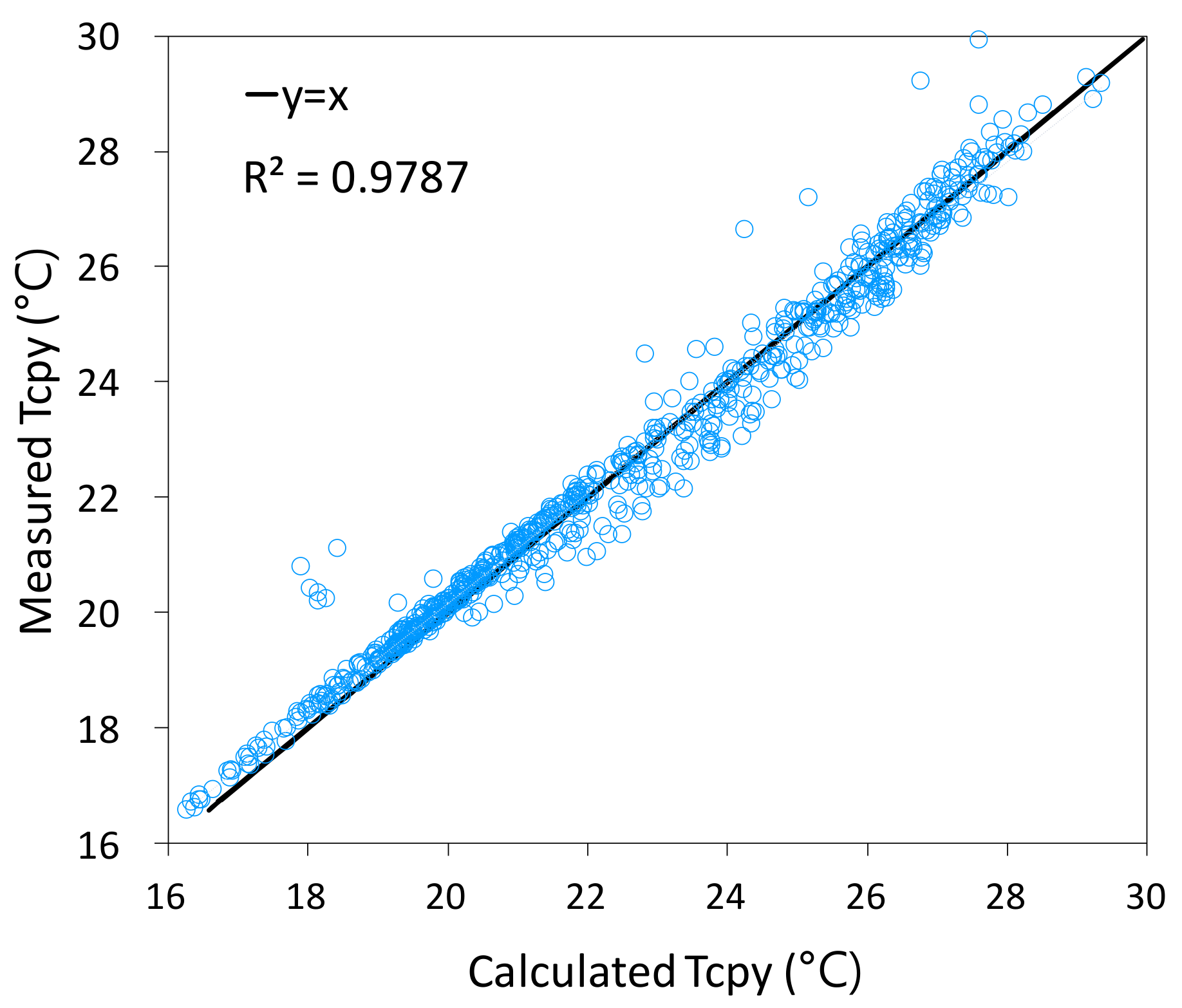
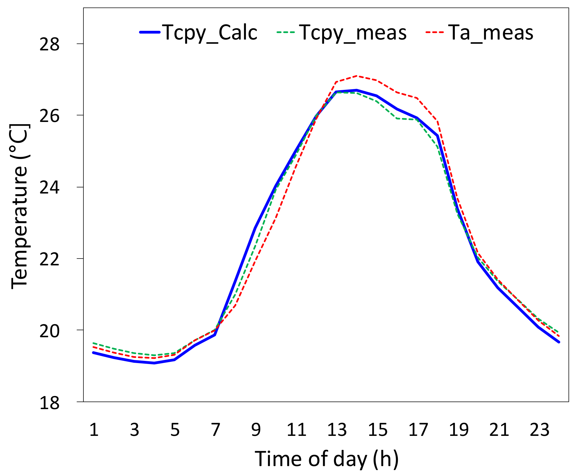
3.2.2. Canopy Temperature and Comparison to Measurements

When calculating the canopy temperature for each LAI for 1 month of the study, the average temperatures of LAI3, LAI2, and LAI1 were 26.1, 25.1, and 24.4 °C, respectively (Figure 11).

To establish a model of the canopy temperature for each LAI, the canopy temperature of an entire LAI was measured with an infrared sensor. For reference, the position where the infrared sensor could be installed was the pole of the other row in the greenhouse, and the field of view of the sensor at that location could capture the entire canopy (Figure 6). The comparison between the model and measurements revealed an accuracy of RMSE 0.457 (Figure 12 and Table 5).

As mentioned earlier, the results of a comparison with the model, measurements of the canopy temperature, and air measurements are shown in Figure 13.

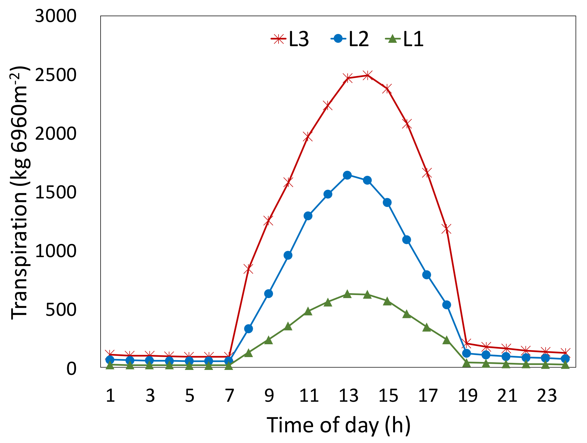
3.2.3. Transpiration

The RMSE of the model for the canopy temperature was discovered to be 0.457. As stated earlier, the equations for the canopy temperature and transpiration could be used alternately, and the transpiration could be estimated accordingly. The absorptivity according to the substrate materials and irrigation volume was excluded from this study. In the event that irrigation was sufficiently supplied, the relationships between the calculated transpiration and the measurements for humidity, irradiation, and CO₂ were as shown in Figure 14.

From the calculations, the transpiration by the LAI can be seen to have been the most active in the shoot apical meristem, which decreased toward the lower canopies (Figure 15). When comparing the transpiration rates between the nighttime and daytime, the difference was observed to be 8.0% in LAI3, 8.1% in LAI2, and 7.2% in LAI1.

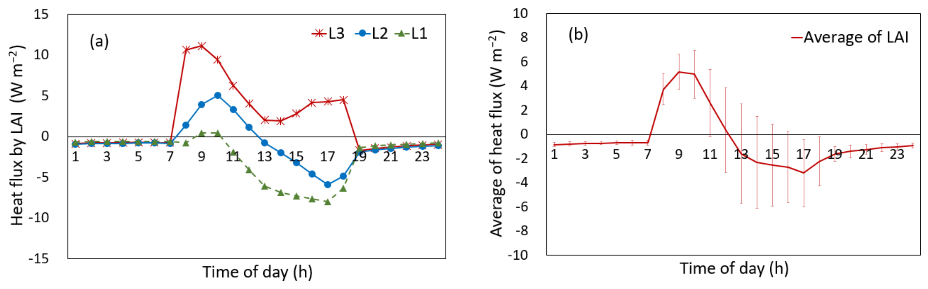
3.2.4. Heat Flux, Impact of Transpiration, and Canopy Temperature

As a consequence of the models for the irradiation, canopy temperature, and transpiration, the heat flux between the canopy and air could be discovered by calculating this from Equations (36)–(40). If the heat flux was positive, the temperature of the canopy was higher than the air temperature, and hence heat must have been released, and if negative, the lower temperature of the canopy absorbed heat from the higher-temperature air. Even during the nighttime, some heat absorption in each LAI was observed (Figure 16).

4. Discussion

The ability to predict transpiration is crucial to understanding the overall physical processes of plants in environmental greenhouses. When transpiration or a corresponding model is obtained, it can be calculated for various types of physical quantities through simple mathematical manipulation. Various transpiration models have been suggested in different types of environments [44]. Among the models mentioned above, the Penman–Monteith model includes a wide range of components to cover the physical properties of crops in greenhouses [45,46,47,48,49]. When it comes to the temperature in a business greenhouse, the air temperature rather than the canopy temperature is generally considered. However, it is necessary to compute the canopy temperature to predict the various interaction models in the greenhouse. Thus, the developed crop model was approached so that the calculated canopy temperature would be taken without requiring a measured canopy temperature. On the other hand, the bell pepper cultivated in a greenhouse has a LAI, and the physical response for each LAI has different characteristics. The effect of including stratified LAI terms in the models was to introduce accurate and sophisticated corrections, which enhanced the interpretation of the plant dynamics. The final results to be obtained through the model equation for the irradiation canopy temperature, transpiration, and heat flux are shown in Figure 10, Figure 11, Figure 12, Figure 13, Figure 14, Figure 15 and Figure 16. We focused our attention on verifying the overall thermal model of bell pepper through high-precision sensors in a Venlo-type greenhouse in South Korea, and an experimental approach was taken to demonstrate the interaction between crops and the climate, accordingly.

4.1. Approximation of Zero Plane Displacement and Roughness Length for Wind Profile

The aerodynamic resistance for partial canopies is related to the plant height (h) and width for crop rows. This causes a change in the sensible heat flux between the LAI and air. Although d and z₀ have an influence on predictions of the wind profile, little information exists on factors determining them for bell pepper, which had a high LAI in the greenhouse. Values of the zero plane displacement (d) and roughness length (z₀) for the experimental crop were selected from previous studies for a variety of canopies. For a sparse cotton field, when the plant height was 0.67 m, z₀ and d were suggested to be 0.36 h and 0.3 h [50]. However, h cannot be the only vegetative characteristic, particularly for sparse crop rows [51]. Authors introduced that d is 0.65 h, z₀ is 0.13 h. z₀ could be increased rapidly early on in the growing season, while d could not be increased significantly for 6 weeks [52]. In our work, we substituted various values of d and z₀ into the wind speed model and found those that caused the canopy temperature measurements and model calculations to give similar results. According to these results, the zero plane displacement was 0.65 h and the roughness lengths (z_M, z_H) for momentum and heat were 0.2 h and 0.3 z_M, respectively. These results are slightly different from those in previous studies, possibly due to the high LAI of bell pepper (2.5), which covered the ground 2.5 times. According to [53], the z₀ is reported to be 0.5 h when the cotton canopy reaches 70% over the ground. In this setting, h is simply related to the canopy height, while z₀ is a more complex function of the canopy structure; the variation of z₀ exhibits a rapid increase as the plants develop.

4.2. Heat Flux by the Temperature Difference between the Canopy and Air

There are few cases where the canopy temperature has been measured or used in South Korean greenhouses. The transpiration model by Stanghellini, developed from the Penman–Monteith equation for the greenhouse environment, includes LAI, but the canopy temperature should be also included. Hence, the Stanghellini model is unlikely to be applicable to greenhouses in South Korea [54]. For this reason, we had to develop a transpiration model that did not require the canopy temperature. Evaporation of water requires large amounts of energy in the forms of heat and radiant energy. Transpiration is governed by energy exchange at the canopy surface, and it is possible to predict the transpiration by applying the principle of energy conservation [55]. The canopy temperature model in this study was obtained by an approximation solution using the linearization technique. Out-emitted, sensible, and latent energies from the canopy surface were calculated by using the air temperature instead of the canopy temperature. Absorbed energies by canopy were also calculated as the air temperature [56]. It was not surprising that the left and right sides of the energy balance equation were exactly the same because of the isothermal condition in which the air and canopy temperatures were considered equal. Although the transpiration model was devised in the above-mentioned way, it was necessary to modify the model to address the heat flux caused by the temperature difference between the canopy and air. Namely, if there was heat loss and gain from the canopy to the air, it was due to non-isothermal conditions. As mentioned when outlining Equations (38)–(42), [32] pointed out how much energy difference occurs between the canopy and air. When calculating Equations (40)–(42), the energy difference obtained from the non-isothermal condition accounted for only ±0.1 to ±2% of the total energy absorbed by the crop. This implies that the plant did not tend to get hot, as it would in isothermal conditions, even when it absorbed strong irradiation.

4.3. Transpiration under the Crop Development Stage in Practice

The crop model developed in this study was developed from the Penman–Monteith equation [57]. The target greenhouse was operating in business and we had limitations in figuring out the irrigation volume. Of course, the water absorption of roots can change according to physicochemical responses such as to the irrigated water temperature, EC (electrical conductivity), cumulated health of roots, etc. [58]. Since our study was not designed to verify the root absorptivity in the substrate, we cannot contend with certainty whether the effect of roots altered the conditions of transpiration. However, the experimental period we studied corresponded to the crop development stage of four growth seasons [55], and this period was mainly for vegetative growth, in which sufficient water must have been irrigating the crops. The calculated results from the transpiration model according to the cultivation for the crop development stage would not have provided a meaningful discrepancy compared to the open water condition. As a result, we found a significant correlation between the calculations and measurements for the canopy temperature (Table 5). As stated in Section 2.2.1, the model of the canopy temperature was the same as that of transpiration.

4.4. Input Variables for Crop Model

Although various crop models in greenhouses are necessary to facilitate the biophysics, especially in South Korea, little research has been conducted on crops suitable for greenhouses such as bell peppers, tomatoes, and strawberries [59,60]. To provide expandable frameworks for future studies, possible variables related to crops and greenhouses were included in our work. The finding that the prediction models for transpiration, canopy temperature, and heat flux per partial canopies have a clear correlation between plants and environmental greenhouses implies that the crop models can allow for management decisions, future yield functions, and greenhouse energy simulations under varied conditions [61,62,63,64]. However, in our work, various input variables were cited from the related literature rather than from measurements of bell peppers, such as the canopy view factor, radiation absorptivity and emissivity, zero plane displacement, and roughness length (Table 3). Even though the computed models were in good agreement with the measurements, the constants of the quoted input variables may have a certain range to compensate for changed values reciprocally. To enhance the accuracy of the cited input variables, future work should develop a measurement method for the bell pepper through statistical-empirical approaches, considering other facts such as pests and diseases [65].

4.5. Regression of Stomatal Vapor Conductance

In Section 2.3.3., various regression models for stomatal vapor conductance under contrasting environmental conditions were examined. Under the condition where the minimum and maximum values of stomatal conductance measurements were 351 and 667 μmol m⁻² s⁻¹, the RMSE, CV (RMSE), and R² in Equation (43) were 84, 0.311, and 0.855, respectively.

Yet, there may have been errors due to the porometer measurement method. The porometer system in our work monitors the relative humidity until the flux gradient reaches a steady state, and measures the diffusive resistance [66]. Of course, it is possible to perform a comparative verification with an IRGA (infrared gas analyzer), but it has been reported that there is no clear information about the two methods [67]. Since the relative humidity in the greenhouse was often over 80%, measurement errors might have occurred due to the calibration over a long period for the diffusive equilibrium [68,69].

We reviewed how the possible errors mentioned above could affect the final result. The accuracy of the canopy temperature was evaluated for the measurements and the regression model of the stomatal conductance. The RMSE, CV (RMSE), and R² of the canopy temperature of LAI3 in the regression model were 0.362, 0.013, and 0.964, respectively. Then, they were 0.273, 0.010, and 0.984 for LAI2, 0.208, 0.008, and 0.988 for LAI1, and 0.272, 0.010, and 0.978 for the mean, respectively.

To improve the accuracy of the stomatal conductance model, a method for extending the measurement period by increasing the quantitative variables, and a method for elaborating on the model through machine learning, could be considered.

4.6. Implication for Modeling the Interactions between Plants and a Field-Based Greenhouse

There could be several directions for extending this work. One obvious direction is to relate it to the photosynthetic function. Our work provides models of how biophysical processes might be assessed. However, application to photosynthetic efficiency would require an appropriate experimental design for not only the aerodynamic resistance and optical response of crops but also the correlation between the transpiration and irrigation volume. The effect of including the above-mentioned factors in the crop model would be to introduce sophisticated corrections where small differences could be better appreciated according to different environments of greenhouses. To obtain the photosynthetic efficiency in future work, it is necessary to consider the light use efficiency (LUE). For the LUE, different radiation characteristics according to each sunlit and shaded area in the canopy should be evaluated, i.e., adding elements such as the intercept and penetrated radiation characteristics to develop an accurate transpiration model [70,71,72,73,74]. Investigation of the photosynthetic efficiency can be carried out through our model, which exhibits the irradiation response per LAI. It will be also desirable to reflect the elements of the greenhouse covering material and screen curtain characteristics in the model, to expand the applicability for each type of greenhouse. Although providing a better yield prediction in the greenhouse industry is a challenging and inevitable problem for future agronomy, this type of work will be increasingly important as information on predicting the physical responses of crops in greenhouses is an expanding need, with the end-goal of better crop management.

5. Conclusions

The irradiation, transpiration, canopy temperature, and heat flux of crops were investigated by the LAI based on the height of the crops in a greenhouse environment. When the LAI was divided into upper, middle, and lower parts for the sunlit and shaded areas, for interception and penetration, compared to the irradiation in LAI3, this was attenuated by 62% in LAI2 and 87% in LAI1. When calculating the transpiration by the LAI, considering the irradiation and environmental greenhouse, compared to LAI3, this was 58% in LAI2 and 23% in LAI1. The RMSE between the model equation and measurements for the canopy temperature was 0.457. By substituting the non-isothermal model of canopy temperature into the isothermal model, it was found that if the canopy temperature was higher than the air temperature, the absorbed energy in the canopy could be calculated as the positive power in Watts, and if it was lower than the air temperature, as the negative power in Watts. The power calculated using this method could be linked to a BES (building energy simulation), such as TRNSYS, EnergyPlus. That simulates the greenhouse heating, and the cooling load and could be a clear reference for the operational method to be used in greenhouses based on the vegetative growth and the reproductive growth strategy, reflected by the LAI. Given the importance of the irradiation, canopy temperature, transpiration, and heat flux modeling, qualitative as well as quantitative improvement of an analytical plant model can contribute significantly to a wide range of improvements in plant growth.

References

1. Kim, H.-J. Effects of Stem Density on Fruit Load; Yield Fluctuation and Production of Sweet Pepper; Graduate School, Chonnam National University: Gwangju, Korea, 2016. [Google Scholar]
2. Joung, K.H.; Jin, H.J.; An, J.U.; Yoon, H.S.; Oh, S.S.; Lim, C.S.; Um, Y.C.; Kim, H.D.; Hong, K.P.; Park, S.M. Analysis of Growth Characteristics and Yield Pattern of ‘Cupra’ and ‘Fiesta’ Paprika for Yield Prediction. Prot. Hortic. Plant Fact. 2018, 27, 349–355. [Google Scholar] [CrossRef]
3. Gupta, S.K.; Ram, J.; Singh, H. Comparative Study of Transpiration in Cooling Effect of Tree Species in the Atmosphere. J. Geosci. Environ. Prot. 2018, 6, 151–166. [Google Scholar] [CrossRef]
4. Lin, H.; Chen, Y.; Zhang, H.; Fu, P.; Fan, Z. Stronger cooling effects of transpiration and leaf physical traits of plants from a hot dry habitat than from a hot wet habitat. Funct. Ecol. 2017, 31, 2202–2211. [Google Scholar] [CrossRef]
5. Van Westreenen, A.; Van Westreenen, A.; Zhang, N.; Zhang, N.; Douma, J.C.; Douma, J.C.; Evers, J.B.; Anten, N.P.R.; Marcelis, L.F.M. Substantial differences occur between canopy and ambient climate: Quantification of interactions in a greenhouse-canopy system. PLoS ONE 2020, 15, e0233210. [Google Scholar] [CrossRef] [PubMed]
6. Albright, L.D.; Seginer, I.; Marsh, L.S.; Oko, A. In situ thermal calibration of unventilated greenhouses. J. Agric. Eng. Res. 1985, 31, 265–281. [Google Scholar] [CrossRef]
7. Tiwari, G.N.; Sharma, P.K.; Goyal, R.K.; Sutar, R.F. Estimation of an efficiency factor for a greenhouse: A numerical and experimental study. Energy Build. 1998, 28, 241–250. [Google Scholar] [CrossRef]
8. Boulard, T.; Baille, A. A simple greenhouse climate control model incorporating effects of ventilation and evaporative cooling. Agric. For. Meteorol. 1993, 65, 145–157. [Google Scholar] [CrossRef]
9. Allen, R.; Smith, M.; Perrier, A.; Pereira, L. An Update for the Definition of Reference Evapotranspiration AND An Update for the Calculation of Reference Evapotranspiration. ICID Bull. Int. Comm. Irrig. Drain. 1994, 43, 1–34. [Google Scholar]
10. Pieters, J.G.; Deltour, J.M. Modelling solar energy input in greenhouses. Sol. Energy 1999, 67, 119–130. [Google Scholar] [CrossRef]
11. Bailey, B.J. Microcliamte, physical processes and greenhouse technology. Acta Hortic. 1985, 174, 35–42. [Google Scholar]
12. Elsner, B.V. Elsner The influence of heating systems on micro climate in crops and possibilities of energy saving. Acta Hortic. 1977, 70, 104–110. [Google Scholar] [CrossRef]
13. Yang, X.; Short, T.H.; Bauerle, W.L. The Microclimate and Transpiration of a Greenhouse Cucumber Crop. Am. Soc. Agric. Eng. 1989, 32, 2143–2150. [Google Scholar] [CrossRef]
14. Raupach, M.R.; Finnigan, J.J. Single-Layer models of evaporation from plant canopies are incorrect but useful, whereas multilayer models are correct but useless: Discuss. Aust. J. Plant Physiol. 1988, 15, 705–716. [Google Scholar] [CrossRef]
15. Demrati, H.; Boulard, T.; Fatnassi, H.; Bekkaoui, A.; Majdoubi, H.; Elattir, H.; Bouirden, L. Microclimate and transpiration of a greenhouse banana crop. Biosyst. Eng. 2007, 98, 66–78. [Google Scholar] [CrossRef]
16. Papadakis, G.; Frangoudakis, A.; Kyritsis, S. Experimental Investigation and Modelling of Heat and Mass Transfer between a Tomato Crop and the Greenhouse Environment. J. Agric. Eng. Res. 1994, 57, 217–227. [Google Scholar] [CrossRef]
17. Yang, X. Greenhouse micrometeorology and estimation of heat and water vapour fluxes. J. Agric. Eng. Res. 1995, 61, 227–238. [Google Scholar] [CrossRef]
18. Morille, B.; Migeon, C.; Bournet, P.E. Is the Penman-Monteith model adapted to predict crop transpiration under greenhouse conditions? Application to a New Guinea Impatiens crop. Sci. Hortic. 2013, 152, 80–91. [Google Scholar] [CrossRef]
19. Katsoulas, N.; Stanghellini, C. Modelling Crop Transpiration in Greenhouses: Different Models for Different Applications. Agronomy 2019, 9, 392. [Google Scholar] [CrossRef]
20. Campbell, G.S.; Norman, J.M. An Introduction to Environmental Biophysics; Springer: Berlin/Heidelberg, Germany, 1998; ISBN 0387949372. [Google Scholar]
21. de Pury, G.G.; Farquhar, G.D. Simple scaling of photosynthesis from leaves to canopies without the errors of big-leaf models. Plant. Cell Environ. 1997, 20, 537–557. [Google Scholar] [CrossRef]
22. Monteith, J.; Unsworth, M. Principles of Environmental Physics: Plants, Animals, and the Atmosphere, 5th ed.; Academic Press: Cambridge, MA, USA, 2013; ISBN 9780123869104. [Google Scholar]
23. Jones, H.G. Plants and Microclimate A Quantitative Approach to Environmental Plant Physiology; Cambridge University Press: Cambridge, UK, 2014. [Google Scholar]
24. Yang, R.; Friedl, M.A. Determination of roughness lengths for heat and momentum over boreal forests. Bound.-Layer Meteorol. 2003, 107, 581–603. [Google Scholar] [CrossRef]
25. Nobel, P.S. Physicochemical and Environmental Plant Physiology, 5th ed.; Academic Press: San Diego, CA, USA, 2020; pp. 1–654. ISBN 978-0-12-819146-0. [Google Scholar]
26. Cionco, R.M. A Mathematical Model for Air Flow in a Vegetative Canopy. J. Appl. Meteorol. Climatol. 1965, 4, 517–522. [Google Scholar] [CrossRef]
27. Oliver, H.R. Wind profiles in and above a forest canopy. Q. J. R. Meteorol. Soc. 1971, 97, 548–553. [Google Scholar] [CrossRef]
28. Goudriaan, J. Crop Micrometeorology a Simulation Study; Wageningen University and Research: Wageningen, The Netherlands, 1977; ISBN 902200614X. [Google Scholar]
29. Bodin, P.; Franklin, O. Efficient modeling of sun/shade canopy radiation dynamics explicitly accounting for scattering. Geosci. Model Dev. 2012, 5, 535–541. [Google Scholar] [CrossRef]
30. Monteith, J. Evaporation and Environment. Symposia of the Society for Experimental Biology. Symp. Soc. Exp. Biol. 1965, 19, 205–234. [Google Scholar]
31. Ou, L.J.; Zhang, Z.Q.; Dai, X.Z.; Zou, X. Photooxidation Tolerance Characters of a New Purple Pepper. PLoS ONE 2013, 8, e63593. [Google Scholar] [CrossRef] [PubMed]
32. Fitter, A.H.; Hay, R.K.M. Environmental Physiology of Plants, 3rd ed.; Academic Press: London, UK, 2002; pp. v–vi. ISBN 978-0-12-257766-6. [Google Scholar]
33. KOZLOWSKI, T.T. Water Deficits and Plant Growth; Academic Press: Cambridge, MA, USA, 1983. [Google Scholar]
34. Ball, J.T.; Wood, I.E.; Berry, J.A. A Model Predicting Stomatal Conductance and its Contribution to the Control of Photosynthesis Under Different Environmental Conditions. Prog. Photosynth. Res. 1987, IV, 221–224. [Google Scholar]
35. Ainsworth, E.A.; Rogers, A. The response of photosynthesis and stomatal conductance to rising [CO2]: Mechanisms and environmental interactions. Plant Cell Environ. 2007, 30, 258–270. [Google Scholar] [CrossRef]
36. Buckley, T.N.; Mott, K.A. Modelling stomatal conductance in response to environmental factors. Plant Cell Environ. 2013, 36, 1691–1699. [Google Scholar] [CrossRef] [PubMed]
37. Caird, M.A.; Richards, J.H.; Donovan, L.A. Nighttime stomatal conductance and transpiration in C3 and C4 plants. Plant Physiol. 2007, 143, 4–10. [Google Scholar] [CrossRef] [PubMed]
38. Shafizadeh, F.; Fu, Y. Pyrolysis Of cellulose. Carbohydr. Res. 1973, 29, 113–122. [Google Scholar] [CrossRef]
39. Fu, Q.S.; Zhao, B.; Wang, Y.J.; Ren, S.; Guo, Y.D. Stomatal development and associated photosynthetic performance of capsicum in response to differential light availabilities. Photosynthetica 2010, 48, 189–198. [Google Scholar] [CrossRef]
40. Knapp, A.K.; Smith, W.K. Stomatal and photosynthetic responses to variable sunlight. Physiol. Plant. 1990, 78, 160–165. [Google Scholar] [CrossRef]
41. Dai, Y.; Dickinson, R.E.; Wang, Y.P. A two-big-leaf model for canopy temperature, photosynthesis, and stomatal conductance. J. Clim. 2004, 17, 2281–2299. [Google Scholar] [CrossRef]
42. Jifon, J.L.; Syvertsen, J.P. Erratum: Moderate shade can increase net gas exchange and reduce photoinhibition in citrus leaves (Tree Physiology 22 (1079–1092)). Tree Physiol. 2003, 23, 719. [Google Scholar] [CrossRef]
43. Heuvelink, T.K.E. Plant Physiology in Greenhouses; Horti-Text: Woerden, The Netherland, 2015; ISBN 9789082332506. [Google Scholar]
44. Ilahi, W.F.F. Evapotranspiration Models in Greenhouse. Master Thesis, Agricultural Bioresearch Engineering, Wageningen University, Wageningen, The Netherlands, 2009; p. 52. [Google Scholar]
45. Kozlov, K.K.; Shaliapin, V.G.; Mamontov, V.V.; Filippov, A.A.; Ostroukhov, N.F.; Korzhuk, M.S.; Pilipenko, A.P. Effect of aerodynamic resistance on energy balance and Penman-Monteith estimates of evapotranspiration in greenhouse conditions. Agric. For. Meteorol. 1992, 58, 209–228. [Google Scholar]
46. Seginer, I. The Penman-Monteith evapotranspiration equation as an element in greenhouse ventilation design. Biosyst. Eng. 2002, 82, 423–439. [Google Scholar] [CrossRef]
47. Willits, D.H. The Penman-Monteith Equation As a Predictor of Transpiration in a Greenhouse Tomato Crop. Soc. Eng. Agric. food, Biol. Syst. 2013, 0300, 034095. [Google Scholar] [CrossRef]
48. Valdés, H.; Ortega-Farias, S.; Argote, M.; Leyton, B.; Olioso, A.; Paillán, H. Estimation of evapotranspiration over a greenhouse tomato crop using the penman-monteith equation. Acta Hortic. 2004, 664, 477–482. [Google Scholar] [CrossRef]
49. Yan, H.; Acquah, S.J.; Zhang, C.; Wang, G.; Huang, S.; Zhang, H.; Zhao, B.; Wu, H. Energy partitioning of greenhouse cucumber based on the application of Penman-Monteith and Bulk Transfer models. Agric. Water Manag. 2019, 217, 201–211. [Google Scholar] [CrossRef]
50. Kustas, W.P.; Choudhury, B.J.; Kunkel, K.E.; Gay, L.W. Estimate of the aerodynamic roughness parameters over an incomplete canopy cover of cotton. Agric. For. Meteorol. 1989, 46, 91–105. [Google Scholar] [CrossRef]
51. Verhoef, A.; McNaughton, K.G.; Jacobs, A.F.G. A parameterization of momentum roughness length and displacement height for a wide range of canopy densities. Hydrol. Earth Syst. Sci. 1997, 1, 81–91. [Google Scholar] [CrossRef]
52. Jacobs, A.F.G.; Van Boxel, J.H. Changes of the displacement height and roughness length of maize during a growing season. Agric. For. Meteorol. 1988, 42, 53–62. [Google Scholar] [CrossRef]
53. Hatfield, J.L. Aerodynamic properties of partial canopies. Agric. For. Meteorol. 1989, 46, 15–22. [Google Scholar] [CrossRef]
54. Stanghellini, C. Transpiration of Greeenhouse Crops an Aid to Climate Management; Institute of Agricultural Engineering (IMAG): Wageningen, The Netherlands, 1987. [Google Scholar]
55. Allen, R.G.; Pereira, L.S.; Raes, D.; Smith, M. Crop Evapotranspiration (Guidelines for Computing Crop Water Requirements); FAO Irrigation and Drainage Paper No. 56; Food and Agriculture Organisation of the United Nations: Rome, Italy, 1998; Volume 300. [Google Scholar]
56. Perera, R.S.; Cullen, B.R.; Eckard, R.J. Using leaf temperature to improve simulation of heat and drought stresses in a biophysical model. Plants 2020, 9, 8. [Google Scholar] [CrossRef] [PubMed]
57. Penman, H.L. Natural evaporation from open water, bare soil and grass. Proc. R. Soc. Lond. Ser. A. Math. Phys. Sci. 1948, 193, 120–145. [Google Scholar]
58. An, S.; Park, S.W.; Kwack, Y. Growth of cucumber scions, rootstocks, and grafted seedlings as affected by different irrigation regimes during cultivation of ‘joenbaekdadagi’ and ‘heukjong’ seedlings in a plant factory with artificial lighting. Agronomy 2020, 10, 1943. [Google Scholar] [CrossRef]
59. Lee, S.-B.; Lee, I.-B.; Homg, S.-W.; Seo, I.-H.; Bitog, P.J.; Kwon, K.-S.; Ha, T.-H.; Han, C.-P. Prediction of Greenhouse Energy Loads using Building Energy Simulation (BES). J. Korean Soc. Agric. Eng. 2012, 54, 113–124. [Google Scholar] [CrossRef]
60. Seong No, L. Design of a Greenhouse Energy Model Including Energy Exchange of Internal Plants and Its Application for Energy Loads Estimation; Seoul National University Graduate School: Seoul, Korea, 2017. [Google Scholar]
61. Chou, S.K.; Chua, K.J.; Ho, J.C.; Ooi, C.L. On the study of an energy-efficient greenhouse for heating, cooling and dehumidification applications. Appl. Energy 2004, 77, 355–373. [Google Scholar] [CrossRef]
62. Van Beveren, P.J.M.; Bontsema, J.; Van Straten, G.; Van Henten, E.J. Minimal heating and cooling in a modern rose greenhouse. Appl. Energy 2015, 137, 97–109. [Google Scholar] [CrossRef]
63. Iddio, E.; Wang, L.; Thomas, Y.; McMorrow, G.; Denzer, A. Energy efficient operation and modeling for greenhouses: A literature review. Renew. Sustain. Energy Rev. 2020, 117, 109480. [Google Scholar] [CrossRef]
64. Kephe, P.N.; Ayisi, K.K.; Petja, B.M. Challenges and opportunities in crop simulation modelling under seasonal and projected climate change scenarios for crop production in South Africa. Agric. Food Secur. 2021, 10, 10. [Google Scholar] [CrossRef]
65. Savary, S.; Teng, P.S.; Willocquet, L.; Nutter, F.W. Quantification and modeling of crop losses: A review of purposes. Annu. Rev. Phytopathol. 2006, 44, 89–112. [Google Scholar] [CrossRef] [PubMed]
66. Bell, C.J.; Squire, G.R. Comparative measurements with two water vapour diffusion porometers (dynamic and steady-state). J. Exp. Bot. 1981, 32, 1143–1156. [Google Scholar] [CrossRef]
67. Toro, G.; Flexas, J.; Escalona, J.M. Contrasting leaf porometer and infra-red gas analyser methodologies: An old paradigm about the stomatal conductance measurement. Theor. Exp. Plant Physiol. 2019, 31, 483–492. [Google Scholar] [CrossRef]
68. Idso, S.B.; Allen, S.G.; Choudhury, B.J. Problems with porometry: Measuring stomatal conductances of potentially transpiring plants. Agric. For. Meteorol. 1988, 43, 49–58. [Google Scholar] [CrossRef]
69. McDermitt, D.K. Sources of Error in the Estimation of Stomatal Conductance and Transpiration from Porometer Data. HortScience 1990, 25, 1538–1548. [Google Scholar] [CrossRef]
70. Lombardini, L.; Restrepo-Diaz, H.; Volder, A. Photosynthetic light response and epidermal characteristics of sun and shade pecan leaves. J. Am. Soc. Hortic. Sci. 2009, 134, 372–378. [Google Scholar] [CrossRef]
71. Lichtenthaler, H.K.; Babani, F.; Navrátil, M.; Buschmann, C. Chlorophyll fluorescence kinetics, photosynthetic activity, and pigment composition of blue-shade and half-shade leaves as compared to sun and shade leaves of different trees. Photosynth. Res. 2013, 117, 355–366. [Google Scholar] [CrossRef]
72. Kim, J.H.; Lee, J.W.; Ahn, T.I.; Shin, J.H.; Park, K.S.; Son, J.E. Sweet pepper (Capsicum annuum L.) canopy photosynthesis modeling using 3D plant architecture and light ray-tracing. Front. Plant Sci. 2016, 7, 1321. [Google Scholar] [CrossRef]
73. Durand, M.; Murchie, E.H.; Lindfors, A.V.; Urban, O.; Aphalo, P.J.; Robson, T.M. Diffuse solar radiation and canopy photosynthesis in a changing environment. Agric. For. Meteorol. 2021, 311, 108684. [Google Scholar] [CrossRef]
74. Zhang, Y.; Yang, J.; Van Haaften, M.; Li, L.; Lu, S.; Wen, W.; Zheng, X.; Pan, J.; Qian, T. Interactions between Diffuse Light and Cucumber (Cucumis sativus L.) Canopy Structure, Simulations of Light Interception in Virtual Canopies. Agronomy 2022, 12, 602. [Google Scholar] [CrossRef]
Figure 1. Aerial photograph of the location of the target greenhouse.
Agronomy 12 01807 g001
Figure 2. Schematic representation of the target greenhouse. Floor plan with air-circulation fan installed is shown in (a). Front, south, and east elevations are depicted in (bd).
Agronomy 12 01807 g002aAgronomy 12 01807 g002b
Figure 3. Line plot adapted with permission from Campbell and Norman, 1998. It depicts the extinction characteristics of diffuse irradiation in the canopy, differing in the leaf angle distribution.
Agronomy 12 01807 g003
Figure 4. Measurements of stomatal conductance in different climate conditions in the greenhouse for 2 days in LAI3. (a) Greenhouse climate measured on 18 September 2021, (b) stomatal conductance at that time, (c) climate measured on 22 September, and (d) conductance at that time, where gvs_ab*, gvs_ad*, gvs_ab, and gvs_ad are the stomatal conductance of the abaxial side in sunlit, adaxial side in sunlit, abaxial side in shade, and adaxial side in shade, respectively.
Agronomy 12 01807 g004
Figure 5. Schematic representing the sensor installation floor plan in the greenhouse. This picture shows sensors for collecting measurements from corners, aisles, and central locations of the greenhouse to assess the representativeness of the greenhouse climate.
Agronomy 12 01807 g005
Figure 6. Schematic depicting the positions of measurements at the upper air height. The vertical position of sensors is given in the elevation view and the horizontal position is given in the floor plan view. Measurements were collected from September to 6 October 2021.
Agronomy 12 01807 g006
Figure 7. Schematic illustrating the sensor installation elevation. The view of the angle of the infrared sensor to measure the surface temperature of the canopy was installed to match the height of the canopy, and the temperature and humidity sensors were located to measure the top and bottom of the canopy with LAI 2.5. Due to the characteristics of the crop rows in the greenhouse, the infrared sensor was installed in the row opposite the other one.
Agronomy 12 01807 g007
Figure 8. Pictures of sensor installation in the greenhouse. Full mount was taken at LAI 1.0 to show the overall installation (a). Temperature, relative humidity, and CO2 sensors of upper air (b), infrared sensor adjusted with view angle (c), and temperature, relative humidity, and CO2 sensors of upper air (d) were installed.
Agronomy 12 01807 g008aAgronomy 12 01807 g008b
Figure 9. Photo representation of the measurement method of LAI. Regarding crop rows in the greenhouse, the probe of the ceptometer extended from the middle of the open space to the mid-row of the crop.
Agronomy 12 01807 g009
Figure 10. Irradiation calculated from Equations (21)–(30): Penetrated and intercepted irradiation through canopy including sunlit and shaded for all components of the beam, scattered diffuse, and scattered beam, where L3 is LAI3, L2 is LAI2, and L1 is LAI1.
Agronomy 12 01807 g010
Figure 11. Canopy temperature calculated from Equation (33). A dependent variable, canopy temperature, is the result of calculations considering all independent variables from Equations (1)–(31) and Table 3. Ta_meas is the measurement of air temperature.
Agronomy 12 01807 g011
Figure 12. Scatterplot of canopy temperatures from model calculations and actual measurements. R2 is the adjusted correlation coefficient.
Agronomy 12 01807 g012
Figure 13. Temperature comparison between model equation and measurements. Tcpy_Calc is the calculated temperature of the canopy, Tcpy_meas are the temperature measurements of the canopy, and Ta_meas are the air temperature measurements.
Agronomy 12 01807 g013
Figure 14. Transpiration (Equation (32)) calculated from 8:00 a.m. to 6:00 p.m. The higher the amount of irradiation, the more the stomatal pores open, whereas the higher the atmospheric humidity and CO2 concentration, the more the stomatal pores closed because the humidity and CO2 level inside the leaf had increased.
Agronomy 12 01807 g014
Figure 15. Calculated transpiration by the leaf area index (LAI). The amount of transpiration is obtained by multiplying the calculated transpiration per unit area by the greenhouse area, as shown. By dividing the transpiration by 90% and multiplying it by the area of the farm, the irrigation volume can be estimated [43].
Agronomy 12 01807 g015
Figure 16. Heat flux between the canopy and air. (a) Heat flux per leaf area index (LAI); (b) average value for LAI3, 2, and 1.
Agronomy 12 01807 g016