Improving the Estimation of Apple Leaf Photosynthetic Pigment Content Using Fractional Derivatives and Machine Learning

Abstract

As a key functional trait, leaf photosynthetic pigment content (LPPC) plays an important role in the health status monitoring and yield estimation of apples. Hyperspectral features including vegetation indices (VIs) and derivatives are widely used in retrieving vegetation biophysical parameters. The fractional derivative spectral method shows great potential in retrieving LPPC. However, the performance of fractional derivatives and machine learning (ML) for retrieving apple LPPC still needs to be explored. The objective of this study is to test the capacity of using fractional derivative and ML methods to retrieve apple LPPC. Here, the hyperspectral data in the 400–2500 nm domains was used to calculate the fractional derivative order of 0.2–2, and then the sensitive bands were screened through feature dimensionality reduction to train ML to build the LPPC estimation model. Additionally, VIs-based ML methods and empirical regression models were developed to compare with the fractional derivative methods. The results showed that fractional derivative-driven ML methods have higher accuracy than the ML methods driven by the original spectra or vegetation index. The results also showed that the ML methods perform better than empirical regression models. Specifically, the best estimates of chlorophyll content and carotenoid content were achieved using support vector regression (SVR) at the derivative order of 0.2 (R² = 0.78) and 0.4 (R² = 0.75), respectively. The fractional derivative maintained a good universality in retrieving the LPPC of multiple phenological periods. Therefore, this study highlights that the fractional derivative and ML improved the estimation of apple LPPC.

1. Introduction

Apples represent one of the most nutritional foods in a healthy diet for their content of water, sugars, organic acids, vitamins, minerals, and dietary fibers [1]. China is the largest apple producer worldwide, producing around 48% of the world’s total production. However, the quality of apples produced in different regions of China varies greatly [2]. Photosynthetic pigments are vital for conserving the energy harnessed by leaf photosynthesis and for growing quality apples. Chlorophyll content (Cab) correlates strongly with the photosynthesis parameters (i.e., the maximum rate of carboxylation measured at a reference temperature (V_cmax25) and the maximum electron transport at a reference temperature (J_max25)), while carotenoid has several functions in photosynthesis, including photon reception and photoprotection [3,4,5,6]. The surface color as an evaluation index of apple quality is determined by the combination of anthocyanins, chlorophyll, and carotenoid (background color) [7].

Optical remote sensing is a reliable method for monitoring the growth status of forests and crops [8,9,10]. Accurate retrieval of structural and biochemical parameters is critical for plant phenotyping. The modeling data sources for the inversion model include hyperspectral, multispectral, and digital data. In recent decades, hyperspectral remote sensing has become a powerful tool for the monitoring of apple leaf photosynthetic pigment content (LPPC, a collective term for Cab and carotenoid content (Cxc) in this paper). For instance, Ta et al. [11] used machine learning to enhance the estimation of apple leaf chlorophyll content from the original hyperspectral data. In addition, Cheng Li et al. [12] developed a vegetation index-based support vector regression (SVR) method to retrieve apple tree canopy chlorophyll content from Sentinel-2A images. Nonetheless, only a few studies have used hyperspectral remote sensing to estimate apple LPPC, and most of the methods have been constructed based on original reflectance or vegetation indices (VIs), which is insufficient for the widely planted apple orchards. Therefore, new methods for retrieving apple LPPC still need to be developed.

There are two typical methods developed to retrieve LPPC, namely physical methods and data-driven methods [13]. Physical methods use the inverse strategies and look-up table generated by radiative transfer models (RTMs) to estimate vegetation parameters. The cost function strategies and the addition of spectral noise both affect the performance of the physical methods [14]. PROSPECT is a widely used leaf optical model in remote sensing inversion and several versions have been developed (i.e., PROSPECT-4, PROSPECT-5, PROSPECT-D) [15]. In addition, other leaf optical models, such as the stochastic model of leaf optical properties (SLOP) [16] and dorsiventral leaf model (DLM) [17], have also been used for the estimation of leaf parameters.

Data-driven methods include empirical regression models and machine learning methods. Empirical regression models based on VIs are widely used due to their simplicity and robustness. A common practice is modeling from the field vegetation parameters (e.g., Cab or leaf area index) and the remote sensing data (e.g., VIs or reflectance) [18]. Most VIs are calculated from the visible, red-edge, and near-infrared spectral domains, such as the widely used normalized difference vegetation index (NDVI), modified chlorophyll absorption ratio index (MCARI), and the double-peak canopy nitrogen index (DCNI) [19]. To monitor the health status, water status, or yield estimate of horticultural crops, numerous studies have been devoted to the application of empirical models based on VIs to the inversion of biophysical parameters. For instance, VIs based on multispectral data from unmanned aerial vehicles were used to estimate tree height and canopy diameter in a pine clonal orchard [20]; the LST-NDVI vegetation index served to estimate tree water status in apple orchards, further informing irrigation strategies [21]; and WorldView satellite imagery was used to map yield in avocado orchards [22]. In addition, multi-platform data has also been used to monitor orchards, for instance, rapid detection of chlorophyll content and distribution in citrus orchards based on low-altitude remote sensing [23], and estimating nitrogen status using canopy and leaf reflectance of red-blush pears [24].

Existing studies show that ML algorithms can accurately estimate the water content, nutritional status, chlorophyll content, and structural parameters of the vegetation [11,25,26]. By training variables and spectral features, the ML methods construct regression models for estimating biophysical parameters [27]. The large number of bands in hyperspectral data may lead to the redundancy of features [28]. To select sensitive features and reduce the dimensionality of the training data, several methods are used, including principal component analysis, Pearson’s correlation coefficient, mean decrease impurity, and variable importance in the projection [29,30,31]. For the training set of ML methods, the VIs, fractional derivative, original spectra, and combinations thereof improve the accuracy of inversion models [32,33,34]. The fractional derivative has been applied to the monitoring of the soil organic matter content [35], nitrogen concentration [34,36], and chlorophyll content [37] of crops due to its ability to enhance spectral properties. However, the performance of fractional derivative-driven ML methods to estimate apple LPPC has not been mentioned, and the transferability of the methods in different phenological periods is also inconclusive.

Therefore, the purposes of this paper are (1) exploring whether the fractional derivative can highlight more detailed features of spectral data, (2) analyzing and filtering sensitive bands with apple LPPC, (3) establishing apple LPPC estimation models and analyzing the performance of different orders and ML methods, and (4) using the most accurate model to retrieve the LPPC of different phenological periods.

2. Materials and Methods

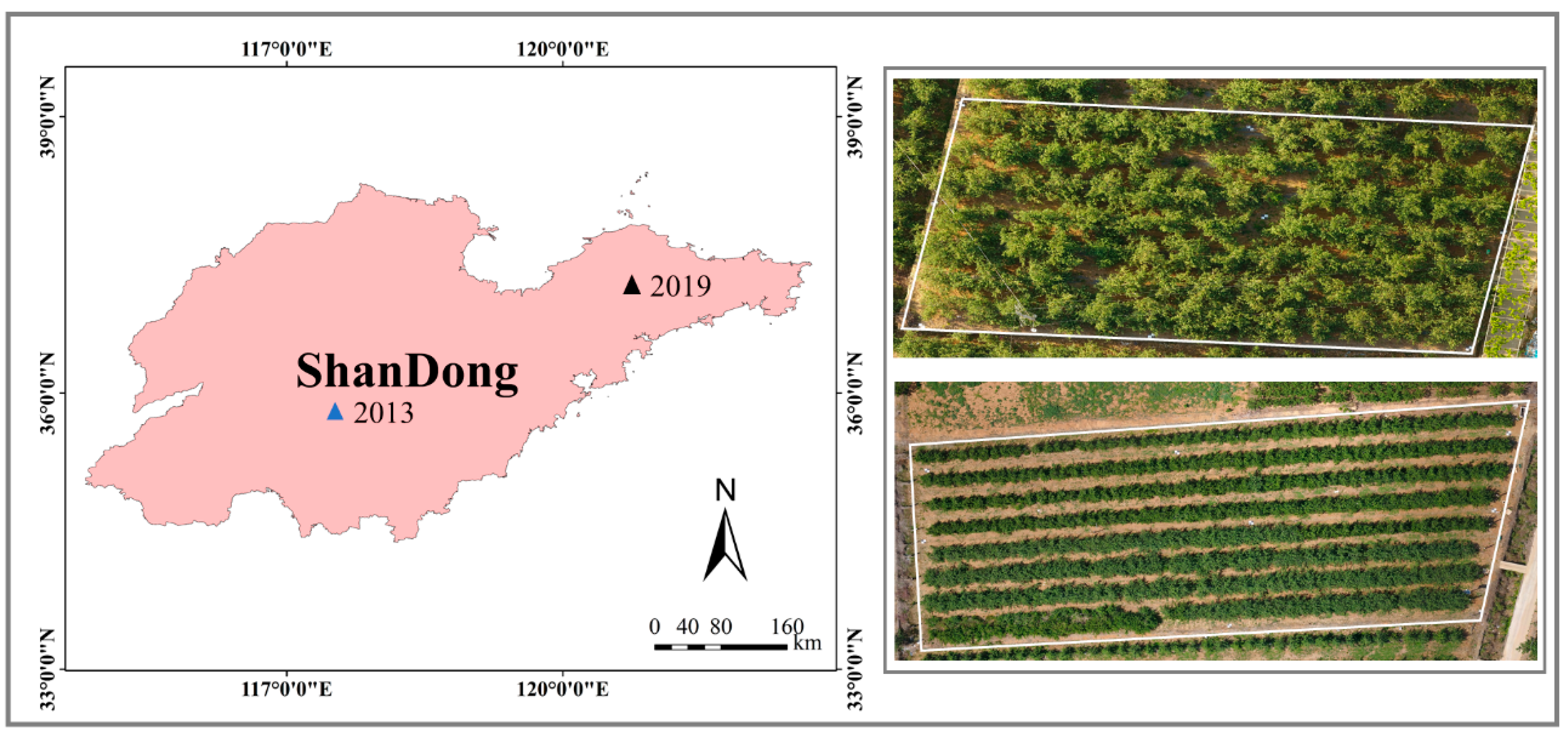
2.1. Study Area

The experiments were carried out in typical Fuji apple orchards in Chaoquan and Guanli towns in Shandong Province, China. The observed data were acquired from the orchards under normal water and fertilizer management. The study areas fall between 36.23–37.27° N and 116.50–120.76° E (Figure 1). The study area has a semi-humid continental monsoon climate, with a mean annual temperature of 11.3 °C and a mean annual precipitation of 650 mm. Moreover, the maximum temperature and rainfall occur in July and August. In addition, the soil in this area is rich in nutrients. Furthermore, during the key phenological periods (from March to October) of apple trees, there is ample sunlight, which greatly improves the energy exchange between the canopy and the environment. Therefore, this area provides abundant water and suitable climatic conditions for the whole growth period of apple trees. The average age of apple orchards is 15 to 25 years, and each tree is separated by 3–5 m.

2.2. Data Acquisition and Preprocessing

The sampling scheme consisted of sampling trees at random in eight orchards of the study district. Field experiments were carried out in five key phenological stages (from April to October in 2013 and 2019), including the flowering stage, fruiting stage, fruit expansion stage, fruit coloring growth stage, and fruit ripening stage. Nine ground observations were carried out and a total of 379 leaf samples were collected from the orchards. The dates and data distribution of the field experiments are shown in

Table 1. Introduction of field experiment dates and the distribution of samples.

Month	Number of Leaves in 2013	Number of Leaves in 2019	Total
April	36	47	83
May	36	97	133
June	36	17	53
September	36	38	74
October	36	-	36
All	180	199	379

. A stratified random sampling strategy was used for trees selection and leaf samples collection; apple leaves were picked at random from the east, south, west, and north of different trees and frozen in a cooler. A single leaf represents a sample for measuring spectral data and LPPC. We took the samples back to the laboratory as soon as possible to prevent a loss of pigment and water content.

2.2.1. Hyperspectral Data Measurements and Preprocessing

The spectral reflectance of the apple leaves was collected by using a Field Spec Pro FR2500 (Analytical Spectral Devices, Boulder, CO, USA). While measuring leaf spectral reflectance, the ASD spectrometer was calibrated using a white reference panel (99%, R value) made of spectral material every half hour. Each leaf sample was scanned ten times using the leaf clip of the ASD spectrometer with a self-contained light source, and the average spectrum was defined as the final value of the leaf sample. This process reduces the impact of noise due to the operation or equipment. The 350–400 nm spectral bands were abandoned because they had considerable signal noise. The reflectance of 2101 bands from 400 to 2500 nm was selected as the spectral data for further study. Although the features in the 350–399 nm bands were abandoned, significant redundant information is available in the 400–2500 nm band that interferes with LPPC inversion.

2.2.2. LPPC Measurements

LPPC was measured chemically in the laboratory by using a Shimadzu UV-2600 spectrophotometer (Shimadzu UV-2600, Kyoto, Japan). During the sampling process, sections of leaves were taken from each leaf sample and then ground and soaked in 80 mL of 95% alcohol until the leaf was white. The spectrophotometer was used to obtain the absorbance at 440, 649, and 665 nm. The following equations were used to calculate the LPPC:

$$\begin{array}{c}chlorophyl{l}_a=\left(13.70\times A_{665}-5.76\times A_{649}\right)\times V_{ml }/L_{a }\end{array}$$

(1)

$$\begin{array}{c}chlorophyl{l}_b=\left(25.80\times A_{649}-7.60\times A_{665}\right)\times V_{ml }/L_{a }\end{array}$$

(2)

$$\begin{array}{c}chlorophyl{l}_{a+b}=chlorophyl{l}_a+chlorophyl{l}_b\end{array}$$

(3)

$$\begin{array}{c}carotenoid=4.70\times A_{440}\times V_{ml }/L_{a }-0.27\times chlorophyl{l}_{a+b}\end{array}$$

(4)

where $chlorophyl{l}_a$ is the chlorophyll-a content, $chlorophyl{l}_b$ is the chlorophyll-b content,$carotenoid$ is the carotenoid content (all in units of $\mathsf{\mu }\mathrm{g}/{\mathrm{cm}}^2$), $V_{ml }$ is 95% of the volume of alcohol, $L_{a }$ is the leaf area of each sample, and $A_{\alpha }$ is the absorbance at the wavelength $\alpha$ (nm).

2.3. Vegetation Indices

In the last decades, simple empirical models based on VI regressions have been pre-dominantly used to estimate Cab and Cxc from hyperspectral data for agricultural monitoring via remote sensing. These approaches are by far the most applied and provide accurate estimates of vegetation biophysical parameters. For this study, 15 common VIs were selected to estimate LPPC (

Table 2. Hyperspectral optical indices used in this study (R in the formula indicates reflectance, numerical values are wavelengths in nm).

VIs	Equation	Reference
Transformed Chlorophyll Absorption in Reflectance Index (TCARI)	$3\times \left[\left(R710-R670\right)-0.2\times \left(R700-R550\right)\left(R710/R670\right)\right]$	[19]
Second Modified Triangular Vegetation Index (MTVI2)	$\frac{1.5\times \left[1.2\times \left(R800-R550\right)-2.5\times \left(R670-R550\right)\right]}{\sqrt{{\left(2\times R800+1\right)}^2-\left(6\times R800-5\sqrt{R670}\right)-0.5}}$	[38]
Double-Peak Canopy Nitrogen Index (DCNI)	$\left(R720-R700\right)/\left(R700-R670\right)/\left(R720-R670+0.03\right)$	[39]
TCARI/Optimized Soil-adjusted Vegetation Index (TCARI/OSAVI)	$\mathrm{TCARI}/[\left(1+0.16\right)\times \left(R800-R670\right)/(R800+R670+0.16)]$	[19]
Modified Chlorophyll Absorption Ratio Index (MCARI)	$\left(R700-R670\right)-0.2\times \left(R700-R550\right)\left(R700/R670\right)$	[19]
Modified Chlorophyll Absorption in Reflectance Index 2 (MCARI2)	$\left(\left(R750-R705\right)-0.2\times \left(R750-R550\right)\right)\times \left(R750/R705\right)$	[40]
MCARI/MTVI2	$\mathrm{MCARI}/\mathrm{MTVI}2$	[41]
MERIS Terrestrial Chlorophyll Index (MTCI)	$\left(R750-R710\right)/\left(R750-R680\right)$	[42]
Normalized Difference Vegetation Index (NDVI)	$\left(R800-R670\right)/\left(R800+R670\right)$	[19]
Green Normalized Difference Vegetation Index (GNDVI)	$\left(R780-R550\right)/\left(R780+R550\right)$	[43]
Normalized Difference Red Edge (NDRE)	$\left(R790-R720\right)/\left(R790+R720\right)$	[44]
Red Edge Chlorophyll Index (CIred_edge)	$R800/R700-1$	[45]
Green Chlorophyll Index (CIgreen)	$R800/R550-1$	[45]
Pigment Specific Simple Ratio Chlorophyll b (PSSRb)	$R800/R650$	[43]
Modified Simple Ratio (MSR)	$\frac{R800/R670-1}{\sqrt{R800/R670+1}}$	[19]

). The indices included simple ratio indices (e.g., pigment-specific simple ratio chlorophyll b (PSSRb)), normalized difference ratios (e.g., NDVI, and normalized difference red edge (NDRE)), and modified vegetation indices based on the existing vegetation indices (e.g., modified chlorophyll absorption in reflectance index 2 (MCARI2)). The 15 VIs used here were not only used to build empirical regression models but were also combined with Cab and Cxc as data sets for ML training.

2.4. Basic Theory of Fractional Derivatives

Fractional derivatives are an effective tool to mine characteristic variables in remote sensing data and are more beneficial to remote sensing modeling than integer derivatives [35]. Grünwald–Letnikov (GL), Riemann–Liouville (RL), and Caputo defined three classical forms of fractional derivative, respectively [46]. Here, we adopt the simple and flexible fractional derivative defined by Grünwald–Letnikov (GL) for spectral transformation, and the formula is as follows:

$$d^{\alpha }f\left(x\right)=\begin{array}{c}\mathrm{l}\mathrm{i}\mathrm{m}\\ h\to 0\end{array}\frac{1}{h^{\alpha }}{\displaystyle \sum }_{m=0}^{\frac{b-a}{h}}{\left(-1\right)}^m\frac{\mathsf{\Gamma }\left(\alpha +1\right)}{m!\mathsf{\Gamma }\left(\alpha -m+1\right)}f\left(x-mh\right)$$

(5)

where $\alpha$ is the order, h is the step length and is set to 1, and b and a are the maximum and minimum of the fractional derivative, respectively. $\mathsf{\Gamma }\left(\alpha \right)$ denotes the Gamma function and the formula is as follows:

$$\mathsf{\Gamma }\left(\alpha \right)={\int }_0^{\infty }\exp \left(-u\right)u^{\alpha -1}du=\left(\alpha -1\right)!.$$

(6)

Then, Formula (5) can be converted to following formula:

$$\frac{d^{\alpha }f\left(x\right)}{d{x}^{\alpha }} \approx f\left(x\right)+\left(-\alpha \right)f\left(x-1\right)+\frac{\left(-\alpha \right)\left(-\alpha +1\right)}{2}f\left(x-2\right)+\cdots \cdots +\frac{\mathsf{\Gamma }\left(-\alpha +1\right)}{n!\mathsf{\Gamma }\left(-\alpha +n+1\right)}f\left(x-n\right)$$

(7)

In this study, to test how the ML methods work with the fractional derivative, we calculated fractional derivative orders starting from 0.2 to 2.0 in increments of 0.2 to explore the accuracy of apple LPPC estimates.

2.5. Selection of Sensitive Features

For any inversion of vegetation biophysical parameters, sensitive features selection of hyperspectral data with a large number of wavelengths is a very important step before using ML methods [1]. Features selection was required before using ML for LPPC inversion [37]. The dimensionality was ideally reduced by using VIs and the sensitive band was selected based on Pearson’s correlation coefficient. A significance level over 0.01 for the relationship between the spectral features and LPPC was defined as a sensitive feature, and then the sensitive features were extracted as training datasets for the ML methods.

2.6. Machine Learning Methods

By analyzing the characteristics of the variables in training datasets, ML methods build relationships between the input variables (e.g., VIs and reflectance) and the biophysical parameters of vegetation (e.g., LAI and Cab). ML algorithms, including SVR, neural networks regression (NNR), partial least squares regression (PLSR), random forest regression (RFR), and K-nearest-neighbor regression (KNNR), were thus applied to estimate apple LPPC from the fractional derivative, VIs, and original reflectance. SVR is a powerful regression tool that is widely used for processing and analyzing remote-sensing data [47]. SVR can handle high and non-normal variables and avoid overfitting the training model [48]. Its main advantage is that it accurately expresses the correlation between variables based on a small sample of data [49]. NNR is a common method for developing nonparametric and nonlinear regression models [50]. NNR imitates the neurons of biological neural networks. Each neuron receives and processes one or more inputs and generates a single output. Training a neural network requires that the characteristics of the network structure (i.e., the number of hidden layers and nodes per layer) be determined and imposes the initial values of parameters and regularization rules to prevent overfitting. Many studies have shown that NNR is useful for retrieving biochemical parameters of crops or forest vegetation [51,52]. In this work, we selected just one hidden layer of neurons and optimized the NNR structure by using the Levenberg–Marquardt learning algorithm with a squared loss function. NNR weights were initialized randomly according to the Nguyen–Widrow method [53]. PLSR builds the regression model on projections obtained by using the partial least squares (PLS) approach. PLSR is often chosen to map vegetation properties. For instance, PLSR is relatively mature for estimating Cab and Cxc based on hyperspectral data and performs well for monitoring the nutrients (e.g., nitrogen, phosphorus, potassium) of fruit trees and other plants [54,55,56]. Some researchers have applied PLSR to map forest structure variables and spatial characteristics (e.g., tree height, canopy diameter, canopy area, and canopy coverage) [26,57,58]. RFR is an ensemble learning technique that uses a set of classification and regression trees (CARTs) to predict unknown variables based on known variables [59]. Two basic parameters need to be determined to use the RFR algorithm: (1) the number of decision trees to be generated (Ntree) and (2) the number of variables to be selected and tested for the best split when growing the trees (Mtry) [60]. KNNR is a multivariate, nonparametric approach to estimation. Implementation of nearest-neighbor techniques requires choices for three parameters: (1) a value for k, the number of nearest neighbors; (2) a scheme for weighting neighbors when calculating predictions; and (3) a distance or similarity metric. The choices are often guided by assessments of results obtained for various combinations of parameters which, in turn, rely on diagnostics related to the quality of predictions, analysis of residuals, extrapolations, inferences, and ease of implementation [61].

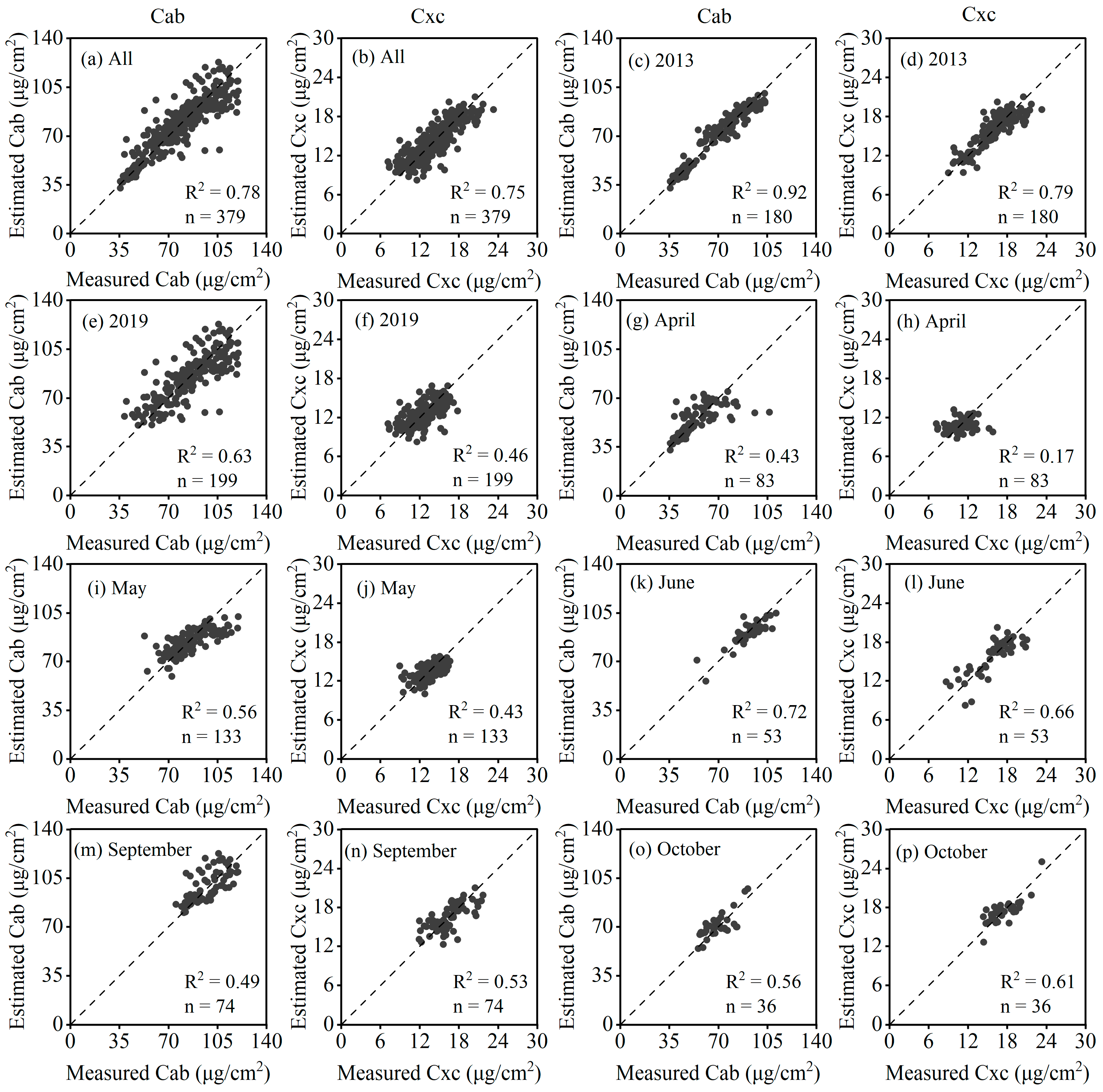
2.7. Model Validation and Accuracy Evaluation

In this study, k-fold was used to validate the estimation models. The basic idea of k-fold is to first divide the dataset into n parts, and then use n−1 parts as the training dataset in turn, and the remaining part as the validation dataset [62]. Here, 10-fold operations were performed, and then the average of the results was calculated as the final estimate of the model. The model performance was evaluated by the root mean squared error (RMSE), coefficient of determination (R²), and normalized RMSE (nRMSE) between the estimated and measured LPPC. The equations are as follows:

$$\begin{array}{c}{R}^2=1-\frac{{{\displaystyle \sum }}_{i=1}^n{(y_i-{\widehat{y}}_i)}^2}{{(y_i-{\overline{y}}_i)}^2}\end{array}$$

(8)

$$\begin{array}{c}RMSE=\sqrt{\frac{{{\displaystyle \sum }}_{i=1}^n{(y_i-{\widehat{y}}_i)}^2}{n}}\end{array}$$

(9)

$$\begin{array}{c}nRMSE=\frac{RMSE}{{\overline{y}}_i}\end{array}$$

(10)

where $i$ = 1, 2, 3, …, n is the validation sample, ${\widehat{y}}_i$ and$y_i$ represent the estimated and measured LPPC values, respectively, and ${\overline{y}}_i$ is the average of each measured variable.

3. Results

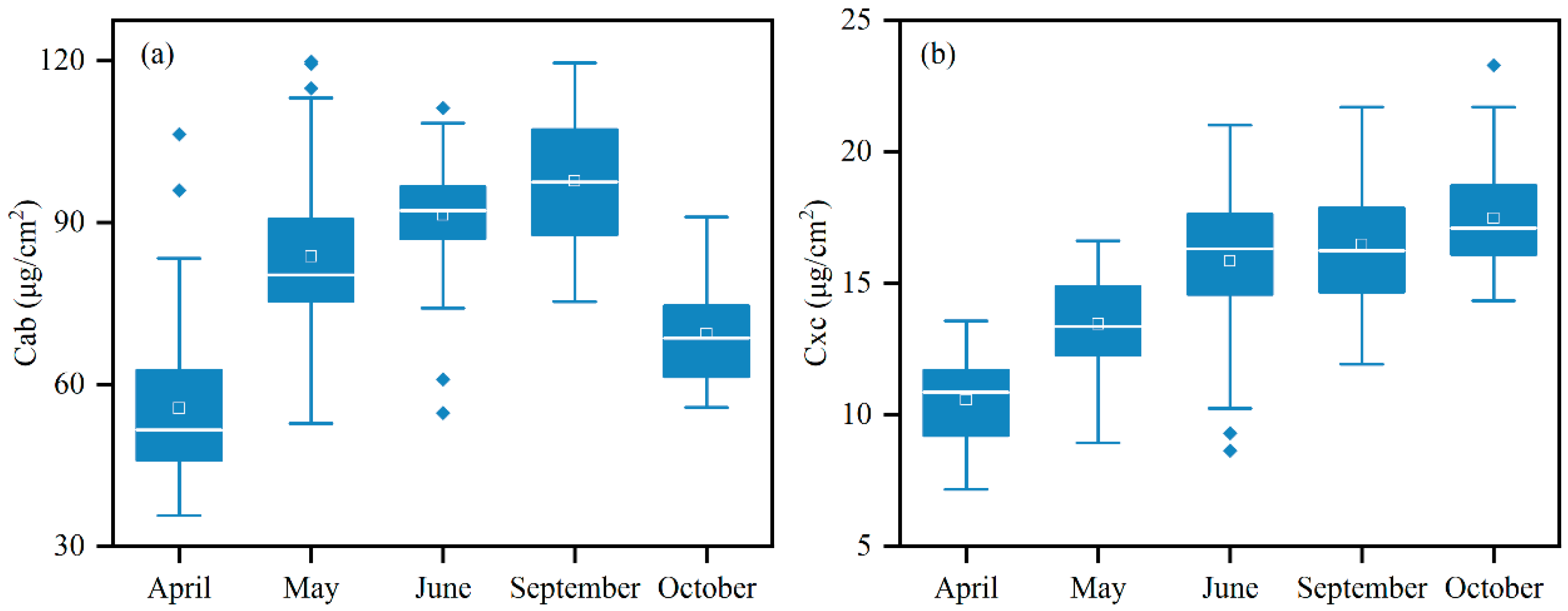
3.1. Descriptive Statistics for the LPPC of Apple Trees

The apple LPPC collected from the field experiments showed great variation. Figure 2 shows the distribution of LPPC over the five growth periods. Cab increased from April to September and suddenly decreased in October; Cxc increased from April to June and kept the same level as June in September and October.

Table 3. Basic statistics of the apple LPPC.

Parameters	Sample Size	Maximum	Minimum	Mean	Standard Deviation	Coefficient of Variation (%)
Cab (μg/cm2)	379	119.87	35.68	80.00	20.39	25.49
Cxc (μg/cm2)	379	23.29	7.17	14.23	2.64	18.55

summarizes the statistics of the field data. The range of Cab was from 35.68 to 119.87 μg/cm², while the range of Cxc was from 7.17 to 23.29 μg/cm². We also found that the changes of Cab and Cxc obviously varied with the seasons.

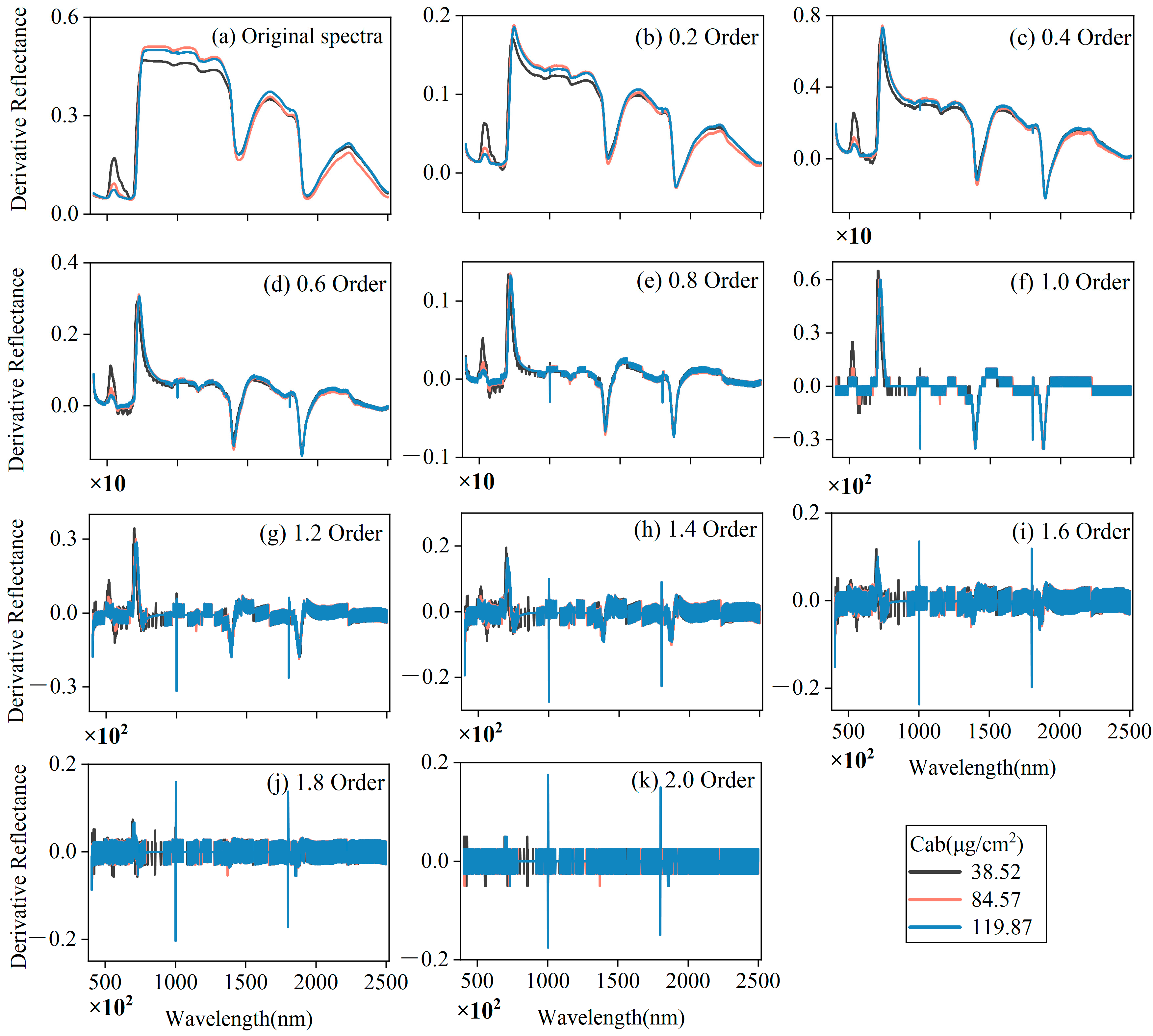
3.2. Spectral Feature of Fractional Derivative

The spectral curves of the measured leaf samples followed similar forms. Figure 3 depicts the original reflectance and fractional derivative for three representative samples. For orders 0.2–1.4, two reflection features appeared near 550 and 730 nm, and three absorption features appeared near 680, 1400, and 1900 nm. Other reflection peaks became sharper in orders 1.6–2.0. Spectral derivative technology not only separated absorption peaks but also magnified weak absorption peaks. With the continuous increase of the differential order, the gap between the maximum value and the minimum value of the differential derivative gradually stabilized from a relatively large dispersion to near zero. Compared with a simple first-order or second-order derivative, the fractional derivative offered richer information. Especially in the visible and red-edge spectral domains, the orders 0.2–1.0 highlighted the number of absorption peaks and reflection peaks, which will be more helpful for us to extract sensitive bands.

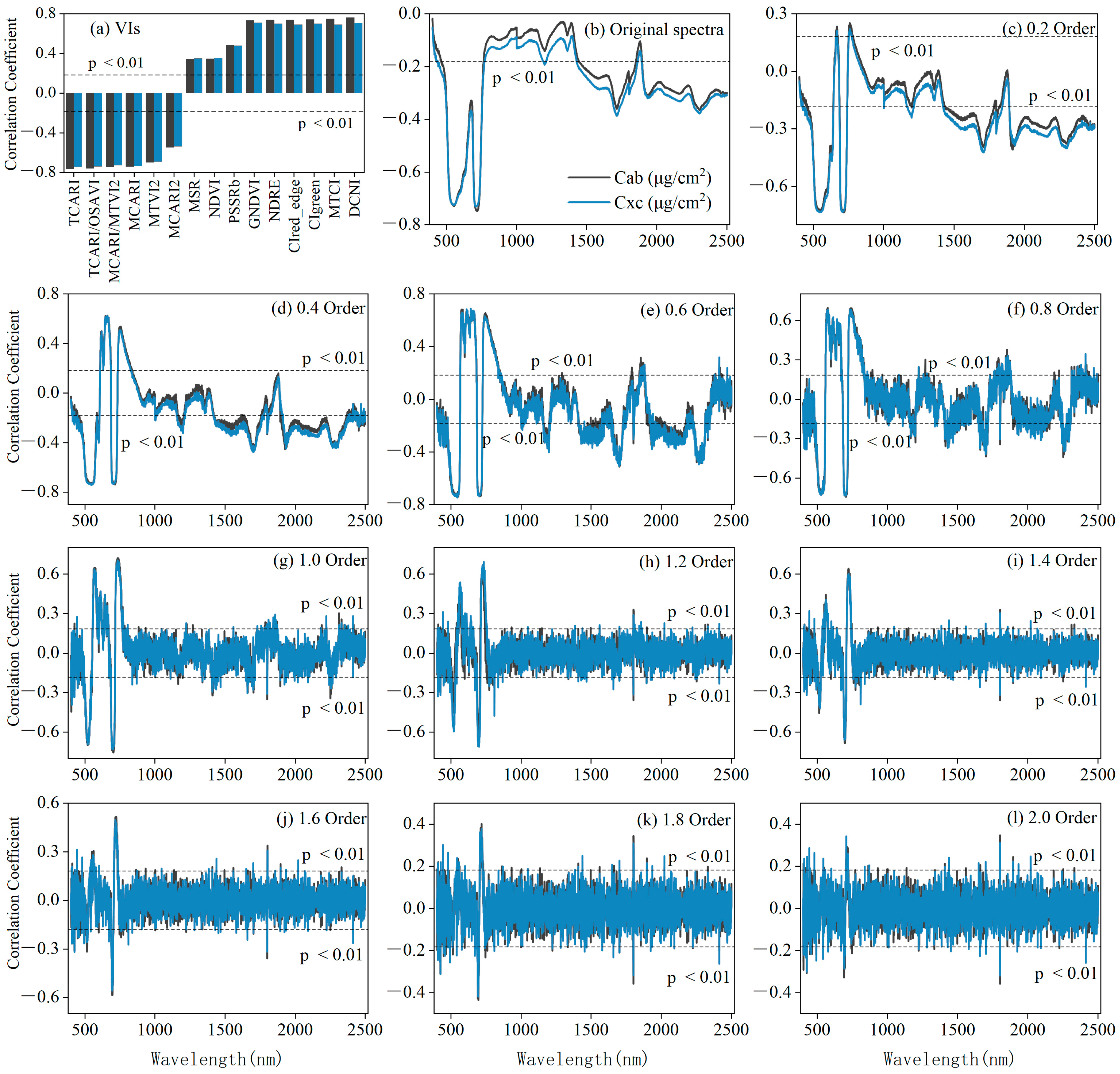
3.3. Sensitive Features Selection

Figure 4 plots Pearson’s correlations for LPPC and VIs, the original spectra, and the fractional derivative orders 0.2–2. The correlation coefficients were tested at the significance level of 0.01. Of the 15 VIs, 6 VIs (TCARI, TCARI/OSAVI, MCARI/MTVI2, MCARI, MTVI2, MCARI2) were negatively correlated and 9 VIs (MSR, NDVI, PSSRb, GNDVI, NDRE, CIred_edge, CIgreen, MTCI, DCNI) were positively correlated. The correlation of each VI to Cab and Cxc was consistent, which means that the correlation of a VI to Cab and Cxc was similar. The LPPC curve from the original spectra or from the fractional derivative orders 0.2–2.0 were consistent. All original spectra were negatively correlated with LPPC, which was particularly strong near 555 and 715 nm (at the 0.01 significance level). Compared with the original spectra, there were multiple positive and negative peaks in the spectral features from orders 0.2 to 1.0, which made it possible to remove the insensitive bands while extracting the sensitive bands, so as to avoid the uncertainty of modeling. For orders 1.2 to 2.0, only a small number of bands in the visible and red-edge spectral domains passed the significance test.

The spectral features that passed the significance test are shown in

Table 4. Statistical analysis of spectral features passing the significance test.

Orders or VIs	Cab			Cxc
	Number of Passing Significance Test	Maximum Value of the Correlation Coefficient	Corresponding VIs or Bands	Number of Passing Significance Tests	Maximum Value of the Correlation Coefficient	Corresponding VIs or Bands
VIs	15	0.76	DCNI	15	0.74	TCARI/OSAVI
Original	1297	0.75	718 nm	1375	0.73	710 nm
0.2	1257	0.74	714 nm	1369	0.73	646 nm
0.4	1304	0.74	714 nm	1366	0.74	546 nm
0.6	1056	0.74	540 nm	1131	0.75	546 nm
0.8	633	0.74	704 nm	681	0.73	700 nm
1.0	327	0.75	704 nm	331	0.73	700 nm
1.2	146	0.68	695 nm	205	0.71	700 nm
1.4	146	0.68	695 nm	145	0.66	694 nm
1.6	96	0.58	697 nm	105	0.56	694 nm
1.8	70	0.43	695 nm	71	0.42	694 nm
2.0	38	0.36	1801 nm	50	0.34	707 nm

Notes: Original denotes the original reflectance.

. Upon increasing the fractional derivative order from 0.2 to 2.0, the general rule was that the number of bands passing the significance test gradually decreased. For orders 0.2–1.0, the number of bands passing the significance test of Cab and Cxc was greater than 300, and a large number of characteristic variables could be obtained; while the number of bands in 1.2–2.0 was less than 200, so some characteristic variables may have been lost. In addition, almost all orders showed that the sensitive bands of LPPC appeared in the visible and red-edge spectral domains. For Cab, the maximum correlation coefficient at 704 nm was 0.75; while for Cxc at 546 nm, the maximum correlation coefficient was 0.75. In addition, the correlation coefficients of order 1.2–2.0 were drastically reduced. Therefore, we extracted more spectral features with higher correlation coefficients in orders 0.2–1.0 than orders 1.2–2.0.

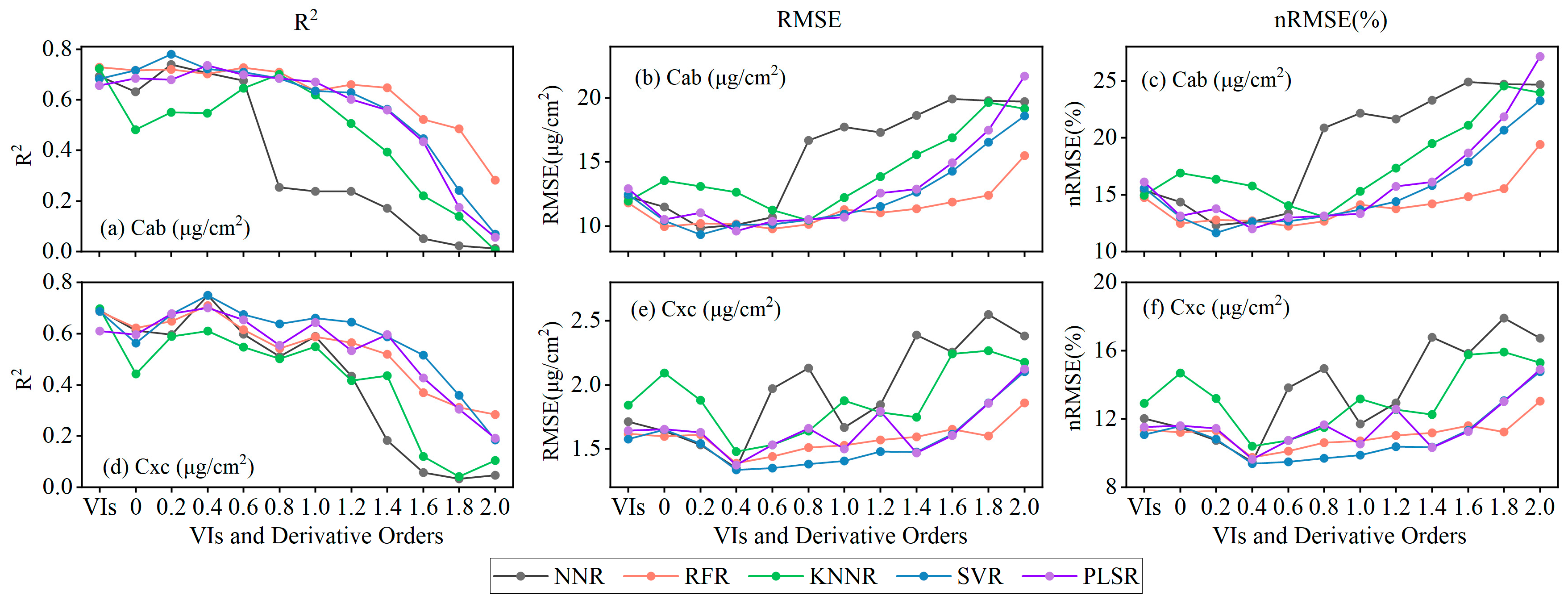
3.4. Performance of Fractional Derivative-Driven ML Methods

Figure 5 shows the R², RMSE, and nRMSE (%) of apple LPPC estimation. For the Cab estimation (Figure 5a–c), SVR, RFR, and PLSR produced the most accurate estimates for fractional derivative orders 0.2–1.0 (R² = 0.64–0.78 and RMSE = 9.33–11.29 μg/cm²). The estimates produced by SVR based on fractional derivative order 0.2 (R² = 0.78, RMSE = 9.33 μg/cm², and nRMSE = 11.66%) was better than those of the other four ML methods. Due to the spectral features becoming subtle and decreasing in number, the models produced inaccurate estimates of LPPC after fractional derivative order 1.0. The results for Cxc (Figure 5d–f) differed slightly from those for Cab. The fractional derivative order 0.4 produced accurate estimates with five ML methods, where SVR obtained the highest precision (R² = 0.75, RMSE = 1.34 μg/cm², nRMSE = 9.42%). The performance of almost all ML methods improved as the order increased to a certain stage, for instance, the SVR estimate of Cxc at the original spectra had R² = 0.56, whereas the most accurate estimate at fractional derivative order 0.4 had R² = 0.75. Overall, the use of the fractional derivative effectively improved the estimation accuracy of LPPC relative to VIs and original reflectance.

To assess the universality of the fractional derivative in different phenological periods and regions, the best models were used to estimate Cab and Cxc (i.e., SVR models of order 0.2 and 0.4), respectively. Since the field trials of the same phenological period in 2013 and 2019 were very close, April, May, June, and September were combined for analysis. The results are shown in Figure 6. Overall, the fractional derivative model estimated Cab and Cxc with good accuracy (R² = 0.78 and 0.75, respectively, Figure 6a,b). For annual validation, the overall accuracy in 2013 was higher than in 2019 (Figure 6c–f). In addition, the model showed a large difference in the robustness of different seasons, and the accuracy was lower than the overall and annual validation, specifically. The model obtained a higher accuracy in May, June, September, and October (R² = 0.43–0.72), while the estimation accuracy of Cxc in April was unsatisfactory (R² = 0.17). The drop in the accuracy of independent validation for seasonality and interannually was mainly caused by the training set, that is, the training of the model did not include interseason and interannual features, resulting in a large gap between the modeling and validation data.

3.5. Comparison with the Empirical Models

In this section, several empirical models developed from VIs were compared with fractional derivative-driven ML methods.

Table 5. Results of validation of empirical models for estimating LPPC.

VIs	Cab (μg/cm2)		Cxc (μg/cm2)
	R2	RMSE	R2	RMSE
TCARI/OSAVI	0.69	11.08	0.71	1.57
NDRE	0.67	12.04	0.66	1.65
DCNI	0.67	11.92	0.68	1.55
TCARI	0.66	12.83	0.65	1.69
MCARI	0.62	12.35	0.56	1.56
MCARI/MTVI2	0.63	12.49	0.56	1.57
MTVI2	0.62	12.55	0.61	1.61
MTCI	0.59	14.79	0.51	1.74
CIred_edge	0.57	14.56	0.50	1.81
CIgreen	0.56	15.29	0.52	1.94
GNDVI	0.56	15.48	0.51	1.97
MCARI2	0.37	17.54	0.29	2.91
PSSRb	0.25	16.34	0.26	2.36
NDVI	0.14	19.68	0.09	4.19
MSR	0.18	22.74	0.12	3.37

shows the inversion results for empirical models based on VIs. Overall, empirical models produced relatively accurate estimates of LPPC. Eleven VIs (i.e., TCARI/OSAVI, NDRE, DCNI, TCARI, MCARI, MCARI/MTVI2, MTVI2, MTCI, CIred_edge, CIgreen, GNDVI) produced accurate estimates of Cab, with R² = 0.56–0.69 and RMSE = 11.08 to 15.48 μg/cm² and, for the accurate estimates of Cxc, with R² = 0.50–0.71 and nRMSE = 1.57–1.97 μg/cm². The remaining models produced inaccurate estimates (R² < 0.4). The linear regression based on TCARI/OSAVI produced the most accurate estimates of all the empirical models for LPPC (Cab: R² = 0.69, RMSE = 11.08 μg/cm²; Cxc: R² = 0.71, RMSE = 1.57 μg/cm²). Overall, it also highlighted the higher accuracy of fractional derivative-driven ML methods compared to empirical models.

4. Discussion

4.1. The Fractional Derivative Improves the Accuracy of LPPC Estimates

Derivative techniques have been widely used for monitoring vegetation parameters [36]. While we used the fractional derivative to enhance the original spectra to obtain more features in this study, the excellent performance of fractional derivative-driven ML was highlighted in the retrieval of LPPC in apple orchards. In addition to using fractional derivatives, VIs were also used as a contrastive strategy to extract feature variables from hyperspectral data. The results showed that it was reasonable to use VIs to build an inversion model, but the accuracy was not significantly improved over the original spectra (Figure 5). Compared to using the integer derivative and VIs as the training data set for ML, using appropriate fractional derivative orders effectively improved the accuracy of LPPC estimation (Figure 5). The main reason for this result was that derivation highlights the subtle features of hyperspectral data and considerably facilitates multiple collinearity problems, so more spectral features were screened, and they contained more information [37]. Fractional differentiation was thus better than integer derivation for processing spectral data. Fractional differentiation of spectral data made better use of the subtle differences between fractional orders to extract features, thereby improving the inversion model [34,35]. For the estimation of Cab and Cxc, the best performing models were at orders 0.2 and 0.4, respectively, which also means that the order of the fractional derivative must be carefully chosen when using this method.

4.2. Universality of the Fractional Derivative

The universality is an important indicator for evaluating the quality of a model. Regional differences pose great challenges to the stability of a model. Although the fractional derivative provided good estimation results, further research should be conducted to evaluate the transferability of the method. The results in Figure 6 showed that in addition to the improved estimation accuracy in 2013, the performance in 2019 and sub-seasons decreased compared to the overall validation. The reason may be that ML methods originated from training datasets that did not fully represent various natural variations, so their performance was inherently limited by the differences of environmental factors [63,64]. Figure 6 clearly showed that the estimation accuracy of LPPC had obvious seasonal variation, which was consistent with the results of Ta et al. [11].

In addition, to further verify the annual transferability, an independent validation was also carried out. Data from 2013 were used for modeling and then validating using data from 2019. The same operation was conducted by swapping the datasets of 2013 and 2019. These results are shown in

Table 6. Interannual validation of LPPC estimates using fractional derivative and ML.

Parameters	2013 Train		2019 Train
	R2	RMSE (μg/cm2)	R2	RMSE (μg/cm2)
Cab (μg/cm2)	0.56	15.52	0.70	12.86
Cxc (μg/cm2)	0.45	2.07	0.48	1.83

. Compared to cross-validation, the estimation accuracy of both Cab and Cxc decreased. The estimation accuracy of Cab (R² = 0.56–0.70, RMSE = 12.86–15.52 μg/cm²) was higher than that of Cxc (R² = 0.45–0.48, RMSE = 1.83–2.07 μg/cm²). A possible reason was that the training samples from a certain period (2013 or 2019) cannot represent the characteristics of the validation data. Every certain period might have its unique dominant disturbing factors. Differences in regional factors (e.g., soil conditions, weather characteristics, or agricultural management) will directly affect the biochemical parameters of apple leaves [65]. In particular, the equivalent water thickness and dry matter content have a very large effect on the spectrum of leaves [13]. Therefore, the instability of environmental factors posed a great challenge to the robustness and transferability of the models. If one wants to improve the estimative ability of the model, the calibration subset data must cover a wide range of samples (e.g., representing multiple stages, temperature characteristics, and soil factors) [64].

4.3. Performance of Different Machine Learning Methods

This paper tested the performance of five ML methods for LPPC estimation and compared them with empirical models based on VIs. ML methods are nonlinear and nonparametric, which allows a relationship model to be built between variables based on the internal characteristics of the data. The ML methods gave more accurate estimate of LPPC than empirical regression models based on VIs. This may have resulted from ML methods using richer spectral features than VI-based empirical models [34,35,36,37]. However, ML methods also required significant preprocessing to estimate LPPC. For instance, the spectrum must be fractionally differentiated to a given order, VIs must be selected, the sensitive features of different fractional reciprocals must be treated, and appropriate training parameters for the ML methods must be selected.

In addition, SVR had outstanding performance in the entire 0.2 to 1.0 orders. This conclusion was also supported by the study of Bhadra et al. [37]. In addition, after order 1.4, the accuracy of almost all models decreased rapidly due to the abrupt reduction of feature variables. Whether it was the estimation of Cab or Cxc, there was difference in performance between multiple ML methods at a certain fractional order. For example, when estimating Cab at order 0.2, the R² of SVR was 0.23 higher than that of KNNR (Figure 5a); when estimating Cxc at order 0.2, the R² of SVR was 0.14 higher than that of KNNR (Figure 5d). Therefore, we recommend carefully screening out high-performance ML methods before implementing this method.

5. Conclusions

In this study, we tested the capacity of using the fractional derivative and ML algorithms to retrieve apple LPPC. We evaluated the universality of the fractional derivative on different phenological periods and the performance of five ML methods on different fractional derivatives. In addition, we also analyzed the accuracy produced by VI-based empirical models and ML methods. In general, fractional derivative-driven ML methods produced more accurate estimates of LPPC than empirical models. Applying appropriate fractional differentiation to spectra improved the performance of the ML methods, with the best being 0.2-order SVR and 0.4-order SVR for estimating Cab and Cxc. The fractional derivative improved the utilization of spectral data, although there were some limitations in different seasons and years, but also maintained a good versatility. In addition, ML had advantages in estimating LPPC, SVR especially provided more accurate LPPC estimation on the orders 0.2–1.0.

This paper highlights the excellent performance of fractional derivative-driven ML methods for LPPC estimation in apple orchards. This method has the potential to map the photosynthetic capacity of crop canopies over large areas. Canopy photosynthetic capacity is key to understanding crop productivity and can be measured by biochemical parameters such as photosynthetic pigments (chlorophyll and carotenoid). Furthermore, photosynthetic pigments are closely related to plant nitrogen content, so they can help growers to dynamically monitor the nutritional status of apple trees to optimize the precise management of orchards and increase fruit productivity.

References

1. Musacchi, S.; Serra, S. Apple fruit quality: Overview on pre-harvest factors. Sci. Hortic. 2018, 234, 409–430. [Google Scholar] [CrossRef]
2. Zhang, Q.; Zhou, B.-B.; Li, M.-J.; Wei, Q.-P.; Han, Z.-H. Multivariate analysis between meteorological factor and fruit quality of Fuji apple at different locations in China. J. Integr. Agric. 2018, 17, 1338–1347. [Google Scholar] [CrossRef]
3. Croft, H.; Chen, J.M.; Luo, X.; Bartlett, P.; Chen, B.; Staebler, R.M. Leaf chlorophyll content as a proxy for leaf photosynthetic capacity. Glob. Chang. Biol. 2017, 23, 3513–3524. [Google Scholar] [CrossRef] [PubMed] [Green Version]
4. Chou, S.; Chen, B.; Chen, J.; Wang, M.; Wang, S.; Croft, H.; Shi, Q. Estimation of leaf photosynthetic capacity from the photochemical reflectance index and leaf pigments. Ecol. Indic. 2020, 110, 105867. [Google Scholar] [CrossRef]
5. Gitelson, A.A.; Gamon, J.A.; Solovchenko, A. Multiple drivers of seasonal change in PRI: Implications for photosynthesis 2. Stand level. Remote Sens. Environ. 2017, 190, 198–206. [Google Scholar] [CrossRef] [Green Version]
6. Zhao, H.; Abulaizi, A.; Wang, C.; Lan, H. Overexpression of CgbHLH001, a Positive Regulator to Adversity, Enhances the Photosynthetic Capacity of Maize Seedlings under Drought Stress. Agronomy 2022, 12, 1149. [Google Scholar] [CrossRef]
7. Lancaster, J.E.; Grant, J.E.; Lister, C.E.; Taylor, M.C. Skin color in apples—influence of copigmentation and plastid pigments on shade and darkness of red color in five genotypes. J. Am. Soc. Hortic. Sci. 1994, 119, 63–69. [Google Scholar] [CrossRef]
8. Li, L.; Ren, T.; Ma, Y.; Wei, Q.; Wang, S.; Li, X.; Cong, R.; Liu, S.; Lu, J. Evaluating chlorophyll density in winter oilseed rape (Brassica napus L.) using canopy hyperspectral red-edge parameters. Comput. Electron. Agric. 2016, 126, 21–31. [Google Scholar] [CrossRef]
9. Darvishzadeh, R.; Skidmore, A.; Schlerf, M.; Atzberger, C.; Corsi, F.; Cho, M. LAI and chlorophyll estimation for a heterogeneous grassland using hyperspectral measurements. ISPRS J. Photogramm. Remote Sens. 2008, 63, 409–426. [Google Scholar] [CrossRef]
10. Noguera, M.; Millan, B.; Aquino, A.; Andújar, J.M. Methodology for Olive Fruit Quality Assessment by Means of a Low-Cost Multispectral Device. Agronomy 2022, 12, 979. [Google Scholar] [CrossRef]
11. Ta, N.; Chang, Q.; Zhang, Y. Estimation of Apple Tree Leaf Chlorophyll Content Based on Machine Learning Methods. Remote Sens. 2021, 13, 3902. [Google Scholar] [CrossRef]
12. Li, C.; Zhu, X.; Wei, Y.; Cao, S.; Guo, X.; Yu, X.; Chang, C. Estimating apple tree canopy chlorophyll content based on Sentinel-2A remote sensing imaging. Sci. Rep. 2018, 8, 3756. [Google Scholar] [CrossRef] [PubMed]
13. Féret, J.-B.; Le Maire, G.; Jay, S.; Berveiller, D.; Bendoula, R.; Hmimina, G.; Cheraiet, A.; Oliveira, J.; Ponzoni, F.J.; Solanki, T. Estimating leaf mass per area and equivalent water thickness based on leaf optical properties: Potential and limitations of physical modeling and machine learning. Remote Sens. Environ. 2019, 231, 110959. [Google Scholar] [CrossRef]
14. Sun, J.; Shi, S.; Wang, L.; Li, H.; Wang, S.; Gong, W.; Tagesson, T. Optimizing LUT-based inversion of leaf chlorophyll from hyperspectral lidar data: Role of cost functions and regulation strategies. Int. J. Appl. Earth Obs. Geoinf. 2021, 105, 102602. [Google Scholar] [CrossRef]
15. Jacquemoud, S.; Baret, F. PROSPECT: A model of leaf optical properties spectra. Remote Sens. Environ. 1990, 34, 75–91. [Google Scholar] [CrossRef]
16. Maier, S.; Lüdeker, W.; Günther, K. SLOP: A revised version of the stochastic model for leaf optical properties. Remote Sens. Environ. 1999, 68, 273–280. [Google Scholar] [CrossRef]
17. Stuckens, J.; Verstraeten, W.W.; Delalieux, S.; Swennen, R.; Coppin, P. A dorsiventral leaf radiative transfer model: Development, validation and improved model inversion techniques. Remote Sens. Environ. 2009, 113, 2560–2573. [Google Scholar] [CrossRef]
18. Sinha, S.K.; Padalia, H.; Dasgupta, A.; Verrelst, J.; Rivera, J.P. Estimation of leaf area index using PROSAIL based LUT inversion, MLRA-GPR and empirical models: Case study of tropical deciduous forest plantation, North India. Int. J. Appl. Earth Obs. Geoinf. 2020, 86, 102027. [Google Scholar] [CrossRef]
19. Wu, C.; Niu, Z.; Tang, Q.; Huang, W. Estimating chlorophyll content from hyperspectral vegetation indices: Modeling and validation. Agric. For. Meteorol. 2008, 148, 1230–1241. [Google Scholar] [CrossRef]
20. Gallardo-Salazar, J.L.; Pompa-García, M. Detecting Individual Tree Attributes and Multispectral Indices Using Unmanned Aerial Vehicles: Applications in a Pine Clonal Orchard. Remote Sens. 2020, 12, 4144. [Google Scholar] [CrossRef]
21. Zare, M.; Drastig, K.; Zude-Sasse, M. Tree water status in apple orchards measured by means of land surface temperature and vegetation index (LST–NDVI) trapezoidal space derived from Landsat 8 satellite images. Sustainability 2020, 12, 70. [Google Scholar] [CrossRef] [Green Version]
22. Wang, K.; Li, W.; Deng, L.; Lyu, Q.; Zheng, Y.; Yi, S.; Xie, R.; Ma, Y.; He, S. Rapid detection of chlorophyll content and distribution in citrus orchards based on low-altitude remote sensing and bio-sensors. Int. J. Agric. Biol. Eng. 2018, 11, 164–169. [Google Scholar] [CrossRef]
23. Robson, A.; Rahman, M.M.; Muir, J. Using worldview satellite imagery to map yield in avocado (Persea americana): A case study in Bundaberg, Australia. Remote Sens. 2017, 9, 1223. [Google Scholar] [CrossRef] [Green Version]
24. Perry, E.M.; Goodwin, I.; Cornwall, D. Remote sensing using canopy and leaf reflectance for estimating nitrogen status in red-blush pears. HortScience 2018, 53, 78–83. [Google Scholar]
25. Muharam, F.M.; Nurulhuda, K.; Zulkafli, Z.; Tarmizi, M.A.; Abdullah, A.N.H.; Che Hashim, M.F.; Mohd Zad, S.N.; Radhwane, D.; Ismail, M.R. UAV-and Random-Forest-AdaBoost (RFA)-based estimation of rice plant traits. Agronomy 2021, 11, 915. [Google Scholar]
26. Reddy, N.; Gebreslasie, M.; Ismail, R. A hybrid partial least squares and random forest approach to modelling forest structural attributes using multispectral remote sensing data. S. Afr. J. Geomat. 2017, 6, 377–394. [Google Scholar]
27. Verrelst, J.; Rivera, J.P.; Gitelson, A.; Delegido, J.; Moreno, J.; Camps-Valls, G. Spectral band selection for vegetation properties retrieval using Gaussian processes regression. Int. J. Appl. Earth Obs. Geoinf. 2016, 52, 554–567. [Google Scholar]
28. Hariharan, S.; Mandal, D.; Tirodkar, S.; Kumar, V.; Bhattacharya, A.; Lopez-Sanchez, J.M. A novel phenology based feature subset selection technique using random forest for multitemporal PolSAR crop classification. IEEE J. Sel. Top. Appl. Earth Obs. Remote Sens. 2018, 11, 4244–4258. [Google Scholar] [CrossRef] [Green Version]
29. Farrés, M.; Platikanov, S.; Tsakovski, S.; Tauler, R. Comparison of the variable importance in projection (VIP) and of the selectivity ratio (SR) methods for variable selection and interpretation. J. Chemom. 2015, 29, 528–536. [Google Scholar] [CrossRef]
30. Li, X.; Zhang, Y.; Bao, Y.; Luo, J.; Jin, X.; Xu, X.; Song, X.; Yang, G. Exploring the best hyperspectral features for LAI estimation using partial least squares regression. Remote Sens. 2014, 6, 6221–6241. [Google Scholar]
31. Li, Z.; Chen, Z.; Cheng, Q.; Duan, F.; Sui, R.; Huang, X.; Xu, H. UAV-Based Hyperspectral and Ensemble Machine Learning for Predicting Yield in Winter Wheat. Agronomy 2022, 12, 202. [Google Scholar] [CrossRef]
32. Prado Osco, L.; Marques Ramos, A.P.; Roberto Pereira, D.; Akemi Saito Moriya, É.; Nobuhiro Imai, N.; Takashi Matsubara, E.; Estrabis, N.; de Souza, M.; Marcato Junior, J.; Gonçalves, W.N.; et al. Predicting Canopy Nitrogen Content in Citrus-Trees Using Random Forest Algorithm Associated to Spectral Vegetation Indices from UAV-Imagery. Remote Sens. 2019, 11, 2925. [Google Scholar] [CrossRef] [Green Version]
33. Sonobe, R.; Sano, T.; Horie, H. Using spectral reflectance to estimate leaf chlorophyll content of tea with shading treatments. Biosyst. Eng. 2018, 175, 168–182. [Google Scholar] [CrossRef]
34. Chen, K.; Li, C.; Tang, R. Estimation of the nitrogen concentration of rubber tree using fractional calculus augmented NIR spectra. Ind. Crop. Prod. 2017, 108, 831–839. [Google Scholar] [CrossRef]
35. Wang, X.; Zhang, F.; Johnson, V.C. New methods for improving the remote sensing estimation of soil organic matter content (SOMC) in the Ebinur Lake Wetland National Nature Reserve (ELWNNR) in northwest China. Remote Sens. Environ. 2018, 218, 104–118. [Google Scholar] [CrossRef]
36. Abulaiti, Y.; Sawut, M.; Maimaitiaili, B.; Chunyue, M. A possible fractional order derivative and optimized spectral indices for assessing total nitrogen content in cotton. Comput. Electron. Agric. 2020, 171, 105275. [Google Scholar] [CrossRef]
37. Bhadra, S.; Sagan, V.; Maimaitijiang, M.; Maimaitiyiming, M.; Newcomb, M.; Shakoor, N.; Mockler, T.C. Quantifying leaf chlorophyll concentration of sorghum from hyperspectral data using derivative calculus and machine learning. Remote Sens. 2020, 12, 2082. [Google Scholar] [CrossRef]
38. Zhou, X.; Zhang, J.; Chen, D.; Huang, Y.; Kong, W.; Yuan, L.; Ye, H.; Huang, W. Assessment of leaf chlorophyll content models for winter wheat using Landsat-8 multispectral remote sensing data. Remote Sens. 2020, 12, 2574. [Google Scholar] [CrossRef]
39. Chen, P.; Haboudane, D.; Tremblay, N.; Wang, J.; Vigneault, P.; Li, B. New spectral indicator assessing the efficiency of crop nitrogen treatment in corn and wheat. Remote Sens. Environ. 2010, 114, 1987–1997. [Google Scholar] [CrossRef]
40. Tahir, M.N.; Naqvi, S.Z.A.; Lan, Y.; Zhang, Y.; Wang, Y.; Afzal, M.; Cheema, M.J.M.; Amir, S. Real time estimation of chlorophyll content based on vegetation indices derived from multispectral UAV in the kinnow orchard. Int. J. Precis. Agric. Aviat. 2018, 1, 24–31. [Google Scholar]
41. Eitel, J.; Long, D.; Gessler, P.; Hunt, E. Combined spectral index to improve ground-based estimates of nitrogen status in dryland wheat. Agron. J. 2008, 100, 1694–1702. [Google Scholar] [CrossRef] [Green Version]
42. Dash, J.; Curran, P. The MERIS terrestrial chlorophyll index. Int. J. Remote Sens. 2004, 25, 5403–5413. [Google Scholar] [CrossRef]
43. Blackburn, G.A. Spectral indices for estimating photosynthetic pigment concentrations: A test using senescent tree leaves. Int. J. Remote Sens. 1998, 19, 657–675. [Google Scholar] [CrossRef]
44. Simic Milas, A.; Romanko, M.; Reil, P.; Abeysinghe, T.; Marambe, A. The importance of leaf area index in mapping chlorophyll content of corn under different agricultural treatments using UAV images. Int. J. Remote Sens. 2018, 39, 5415–5431. [Google Scholar] [CrossRef]
45. Gitelson, A.A.; Viña, A.; Ciganda, V.; Rundquist, D.C.; Arkebauer, T.J. Remote estimation of canopy chlorophyll content in crops. Geophys. Res. Lett. 2005, 32, L08403. [Google Scholar] [CrossRef] [Green Version]
46. Benkhettou, N.; da Cruz, A.M.B.; Torres, D.F. A fractional calculus on arbitrary time scales: Fractional differentiation and fractional integration. Signal Process. 2015, 107, 230–237. [Google Scholar] [CrossRef] [Green Version]
47. Verrelst, J.; Camps-Valls, G.; Muñoz-Marí, J.; Rivera, J.P.; Veroustraete, F.; Clevers, J.G.; Moreno, J. Optical remote sensing and the retrieval of terrestrial vegetation bio-geophysical properties–A review. ISPRS J. Photogramm. Remote Sens. 2015, 108, 273–290. [Google Scholar] [CrossRef]
48. Ge, J.; Meng, B.; Liang, T.; Feng, Q.; Gao, J.; Yang, S.; Huang, X.; Xie, H. Modeling alpine grassland cover based on MODIS data and support vector machine regression in the headwater region of the Huanghe River, China. Remote Sens. Environ. 2018, 218, 162–173. [Google Scholar] [CrossRef]
49. Siegmann, B.; Jarmer, T. Comparison of different regression models and validation techniques for the assessment of wheat leaf area index from hyperspectral data. Int. J. Remote Sens. 2015, 36, 4519–4534. [Google Scholar] [CrossRef]
50. Kubat, M. Neural networks: A comprehensive foundation by Simon Haykin, Macmillan, 1994, ISBN 0-02-352781-7. Knowl. Eng. Rev. 1999, 13, 409–412. [Google Scholar] [CrossRef]
51. Danner, M.; Berger, K.; Wocher, M.; Mauser, W.; Hank, T. Efficient RTM-based training of machine learning regression algorithms to quantify biophysical & biochemical traits of agricultural crops. ISPRS J. Photogramm. Remote Sens. 2021, 173, 278–296. [Google Scholar]
52. Ali, A.M.; Darvishzadeh, R.; Skidmore, A.; Gara, T.W.; Heurich, M. Machine learning methods’ performance in radiative transfer model inversion to retrieve plant traits from Sentinel-2 data of a mixed mountain forest. Int. J. Digit. Earth 2021, 14, 106–120. [Google Scholar] [CrossRef]
53. Caicedo, J.P.R.; Verrelst, J.; Muñoz-Marí, J.; Moreno, J.; Camps-Valls, G. Toward a semiautomatic machine learning retrieval of biophysical parameters. IEEE J. Sel. Top. Appl. Earth Obs. Remote Sens. 2014, 7, 1249–1259. [Google Scholar] [CrossRef]
54. Mahajan, G.R.; Das, B.; Murgaokar, D.; Herrmann, I.; Berger, K.; Sahoo, R.N.; Patel, K.; Desai, A.; Morajkar, S.; Kulkarni, R.M. Monitoring the foliar nutrients status of mango using spectroscopy-based spectral indices and PLSR-combined machine learning models. Remote Sens. 2021, 13, 641. [Google Scholar] [CrossRef]
55. Flynn, K.C.; Frazier, A.E.; Admas, S. Nutrient prediction for tef (Eragrostis tef) plant and grain with hyperspectral data and partial least squares regression: Replicating methods and results across environments. Remote Sens. 2020, 12, 2867. [Google Scholar] [CrossRef]
56. Meacham-Hensold, K.; Montes, C.M.; Wu, J.; Guan, K.; Fu, P.; Ainsworth, E.A.; Pederson, T.; Moore, C.E.; Brown, K.L.; Raines, C. High-throughput field phenotyping using hyperspectral reflectance and partial least squares regression (PLSR) reveals genetic modifications to photosynthetic capacity. Remote Sens. Environ. 2019, 231, 111176. [Google Scholar] [CrossRef]
57. Wolter, P.T.; Townsend, P.A.; Sturtevant, B.R. Estimation of forest structural parameters using 5 and 10 meter SPOT-5 satellite data. Remote Sens. Environ. 2009, 113, 2019–2036. [Google Scholar] [CrossRef]
58. Shi, Z.; Ai, L.; Li, X.; Huang, X.; Wu, G.; Liao, W. Partial least-squares regression for linking land-cover patterns to soil erosion and sediment yield in watersheds. J. Hydrol. 2013, 498, 165–176. [Google Scholar] [CrossRef]
59. Breiman, L. Random forests. Mach. Learn. 2001, 45, 5–32. [Google Scholar] [CrossRef] [Green Version]
60. Belgiu, M.; Drăguţ, L. Random forest in remote sensing: A review of applications and future directions. ISPRS J. Photogramm. Remote Sens. 2016, 114, 24–31. [Google Scholar] [CrossRef]
61. McRoberts, R.E.; Næsset, E.; Gobakken, T. Optimizing the k-Nearest Neighbors technique for estimating forest aboveground biomass using airborne laser scanning data. Remote Sens. Environ. 2015, 163, 13–22. [Google Scholar] [CrossRef]
62. Fushiki, T. Estimation of prediction error by using K-fold cross-validation. Stat. Comput. 2011, 21, 137–146. [Google Scholar] [CrossRef]
63. Sagan, V.; Peterson, K.T.; Maimaitijiang, M.; Sidike, P.; Sloan, J.; Greeling, B.A.; Maalouf, S.; Adams, C. Monitoring inland water quality using remote sensing: Potential and limitations of spectral indices, bio-optical simulations, machine learning, and cloud computing. Earth-Sci. Rev. 2020, 205, 103187. [Google Scholar] [CrossRef]
64. Zeng, L.; Chen, C. Using remote sensing to estimate forage biomass and nutrient contents at different growth stages. Biomass Bioenergy 2018, 115, 74–81. [Google Scholar] [CrossRef]
65. Houborg, R.; McCabe, M.F. A hybrid training approach for leaf area index estimation via Cubist and random forests machine-learning. ISPRS J. Photogramm. Remote Sens. 2018, 135, 173–188. [Google Scholar] [CrossRef]
Figure 1. Location of study areas and schematic of drone digital images of the apple orchards. The blue and black triangles in the figure are the ground sampling points in 2013 and 2019, respectively.
Agronomy 12 01497 g001
Figure 2. Distribution of LPPC in five phenological periods. Panel (a) and (b) show the distribution of Cab and Cxc from April to October, respectively.
Agronomy 12 01497 g002
Figure 3. Features of the minimum, median, and maximum LPPC samples produced by fractional derivation of the original spectra. Panel (a) shows the original spectra, and the remaining panels (bk) show the fractional derivative orders 0.2–2.
Agronomy 12 01497 g003
Figure 4. Pearson’s correlations between LPPC and VIs, original spectra, and fractional derivative orders in the validation dataset.
Agronomy 12 01497 g004
Figure 5. R2, RMSE, and nRMSE (%) of estimated LPPC based on VIs, original spectra, and fractional derivative orders. Order zero on the x axis is the original spectra.
Agronomy 12 01497 g005
Figure 6. Model performance in LPPC estimates for different phenological periods. (a,b) are the validation of Cab and Cxc for all samples, respectively. (cf) are the validation of Cab and Cxc in 2013 and 2019, respectively. (gp) are the validation of Cab and Cxc from April to October, respectively.
Agronomy 12 01497 g006