Wavelet Decomposition and Machine Learning Technique for Predicting Occurrence of Spiders in Pigeon Pea

Abstract

Influence of weather variables on occurrence of spiders in pigeon pea across locations of seven agro-climatic zones of India was studied in addition to development of forecast models with their comparisons on performance. Considering the non-normal and nonlinear nature of time series data of spiders, non-parametric techniques were applied with developed algorithm based on combinations of wavelet–regression and wavelet–artificial neural network (ANN) models. Haar wavelet filter decomposed each of the series to extract the actual signal from the noisy data. Prediction accuracy of developed models, viz., multiple regression, wavelet–regression, and wavelet–ANN, tested using root mean square error (RMSE) and mean absolute percentage error (MAPE), indicated better performance of wavelet–ANN model. Diebold Mariano (DM) test also confirmed that the prediction accuracy of wavelet–ANN model, and hence its use to forecast spiders in conjunction with the values of pest–defender ratios, would not only reduce insecticidal sprays, but also add ecological and economic value to the integrated pest management of insects of pigeon pea.

1. Introduction

Pigeon pea (Cajanus cajan (L.) Millsp.), often known as red gram, is an important legume crop grown in tropical and subtropical areas of the world. Pigeon pea is grown in over 25 countries worldwide across approximately 4.59 million hectares, with its output near to 3.25 million tonnes. Pigeon pea is planted on 5.6 million hectares in India, with an annual production of 3.29 million tonnes [1,2] and productivity of 587 kg/ha, lower than the world average of 695 kg/ha. Pigeon pea in India is grown across the states of Maharashtra, Karnataka, Madhya Pradesh, Gujarat, Uttar Pradesh, and Telangana. Pigeon pea productivity is affected by biotic and abiotic factors under Indian settings [3]. Among biotic factors, yield loss due to major insects range from 27 percent to 100 percent [4,5,6,7], of which lepidopterous insects such as Grapholita critica (Meyr.), Tortricidae, spotted pod borer, Maruca vitrata (Fabricius), and gram pod borer Helicoverpa armigera (Hubner) are important feeders on foliage and reproductive (flower and pod) structures. Sucking insects, mainly jassids, have attained pest status in the current decade. Eight spider species preying on Helicoverpa armigera larvae, the major pod borer in pigeon pea, and their role in suppression of variety of other insects of the sucking and chewing feeding category is well-recognized [8,9]. Spiders are general predators present in almost all agro-ecosystems that help to control jassids, aphids, thrips, mites, and the eggs of numerous insect pests [10], thus offering native natural control. In diverse pigeon pea agro-ecosystems, climate considerations also have an impact on spider populations and their dynamics [11]. Hence, prediction of spider populations in relation to weather using appropriate models would aid in strategizing pest management in pigeon pea ecosystems.

Weather-based relationships and prediction of spiders as predators would aid farmers in making appropriate pest-control decisions. However, to correctly anticipate spider dynamics, it is necessary to utilize precise and trustworthy algorithms to analyze the data with environmental parameters. The autoregressive integrated moving average (ARIMA) model [12] uses a series’ inherent inertia to anticipate future values. In the realm of agriculture, time series models like ARIMA and ARIMA with exogenous variables (ARIMAX) models are used to forecast agricultural prices [13,14,15]. However, there are not many applications of these models for forecasting insects of pest/predator/parasitoid categories. The ARIMAX model was used [16,17] to predict insect populations [18], wherein machine learning techniques were used. For forecasting insects and diseases of various crops, the LR, ARIMA model, and ANN architecture have been widely used in the literature [19,20]. The algorithm combining wavelet decomposition followed by application of machine learning techniques has been developed for its effective use in time series forecasting of commodity prices and rainfall [21,22]. Machine learning techniques were also used to study pest population dynamics [17]. In Central America, machine learning approaches were used to forecast Sigatoka illness in banana and plantain crops [23]. An attempt has been made in the present study to combine wavelets with regression and ANN to forecast the occurrence of spiders at seven different locations of India in diverse climatic zones and eco regions. The hypothesis that the developed model’s accuracy in forecasting spiders is better than the standard regression model was also investigated.

2. Methodology

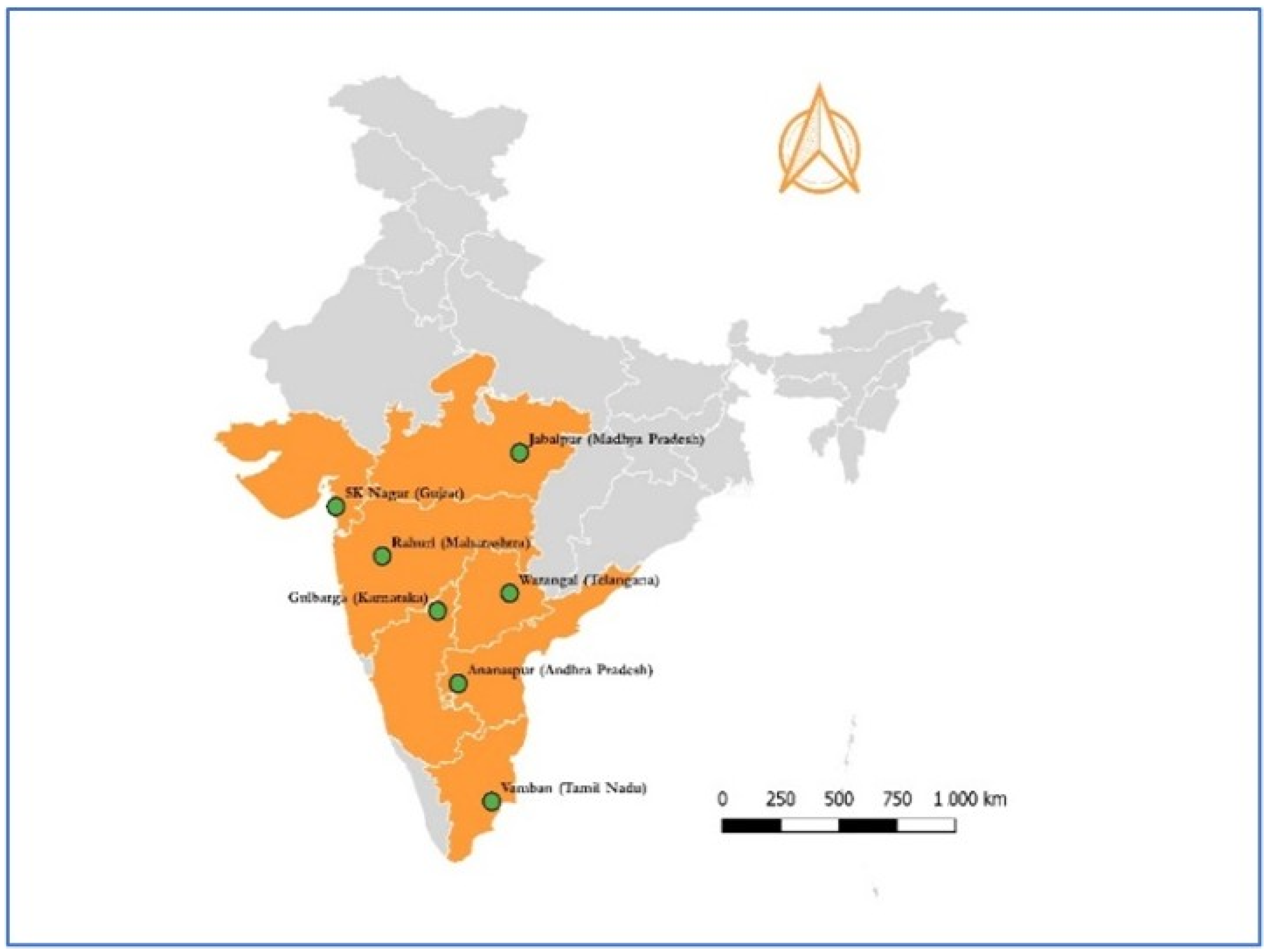
2.1. Study Locations, Surveillance, and Sampling Plans for Spiders and Weather

Seven pigeon-pea-growing locations belonging to different agro-climatic zones, regions, and states were considered and the same is displayed in Figure 1. The study was part of a mega-program on the ‘study of pest dynamics in relation to climate change’ under the ‘National Innovations in Climate Resilient Agriculture (NICRA)’ that has used information and communication technology (ICT) for database development and reporting. Ten villages in each study location during each season (number of seasons varied with study locations between 2011 and 2017) with two pigeon pea farms each with a minimum of one acre (4000 sq·m) in a village selected for surveillance, including spider surveillance. Sowing dates by location and season were dependent on onset of monsoon (post rains). A standard package of practices recommended for pigeon pea cultivation in terms of cultivars, intercultural operations, de-weeding, fertilization, and need-based management of insects and diseases were followed in each of the study locations. Spiders (both spiderlings and adults), largely constituted by Araneus sp. and Clubiona sp., were counted together on a single plant (whole plant basis) per spot, with five such spots selected randomly in each farm following a sampling interval of a week from vegetative crop stage until harvesting. The mean number of spiders per plant formed the point data for a particular week per farm. It is to be mentioned that sample farms were selected, for all locations and seasons, from within a 30 km radius from a meteorological observatory at the study location. Weather data relating to the study seasons on a standard meteorological week (SMW) basis corresponding to the dynamics of spiders during 2011–2017 were considered in the study.

Graphical representation and descriptive statistics on the time series data (seasonality) of spiders were made, in addition to deducing the range of prevalent weather over seasons (2011–2017) of individual study locations. Influence of weather on spider population dynamics over aggregated seasons were worked out through correlative analysis. Models, viz., linear regression (LR), wavelet in combination with regression, and ANN models, were used to predict spider occurrence. The RMSE, MAPE, and Diebold Mariano test [24] were utilized to make comparisons of predictive performance. A brief description of the methodology of models used is given below.

2.2. Multiple Linear Regression Model

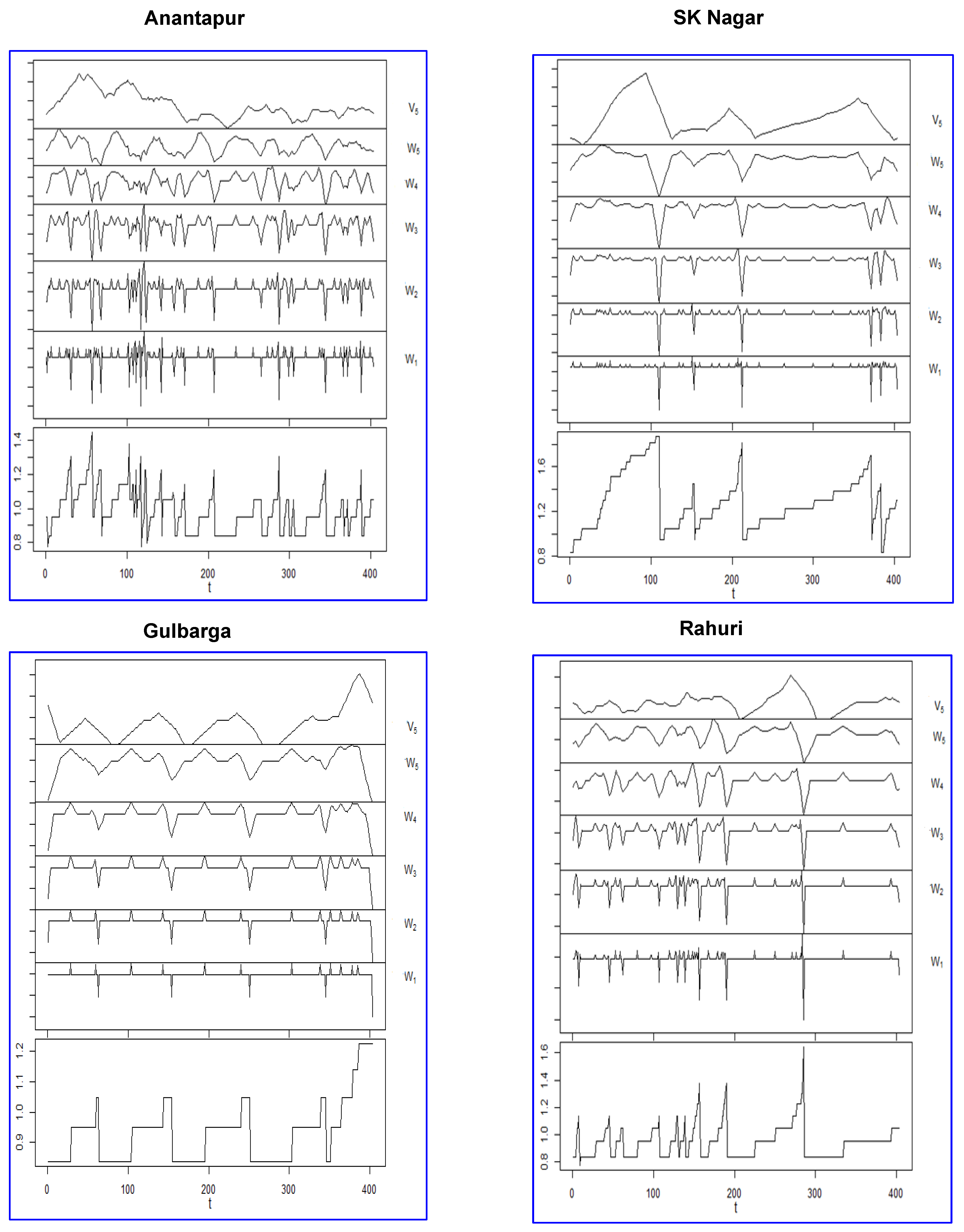
Let us assume that data consist of $N$ observations of response variable $Y$ and $p$ predictors, $X_1,X_2,\dots ,X_p$. The relationship between $Y$ and $X_1,X_2,\dots ,X_p$ is formulated as a linear model

$$Y={\beta }_0+{\beta }_1{X}_1+\dots +{\beta }_p{X}_p+\epsilon .$$

where ${\beta }_0,{\beta }_1,\dots {\beta }_p$ are constants referred to as the regression coefficients and $\epsilon$ is a random disturbance or error which is assumed to follow the normal distribution with mean zero and a constant variance. It is assumed that $Y$ is a linear function of $X$, and the disparity in that approximation is measured [25]. The most widely-used selection techniques for selecting the important variables in the model are Forward, Backward, and Stepwise selection. The significant variables in the model were chosen using a stepwise selection process in the current study.

2.3. Wavelets

Assuming that, $\psi (.)$ is a real-valued function defined on $\left(-\infty ,\infty \right)$ and it satisfies the properties: (i)${{\displaystyle \int }}_{-\infty }^{\infty }\psi \left(u\right) \mathrm{du} =0$ and (ii) ${{\displaystyle \int }}_{-\infty }^{\infty }{\psi }^2\left(u\right) \mathrm{du} =1$, then the function $\psi (.)$ is called a wave. The details of wavelets and their application in time series can be found in [26,27,28].

There are mainly two types of wavelet transform: (i) continuous wavelet transform (CWT), designed to work with series defined on $\left(-\infty ,\infty \right)$; (ii) discrete wavelet transform (DWT) which deals with series defined essentially over a range of integers. DWT is used to capture high- and low-frequency components of a signal which, in turn, would enable modeling of series through computation of inverse DWT. However, DWT requires length of time series ($N$) to be a multiple of 2^J, where J is a positive integer and denotes of the level of decomposition. Therefore, the maximal overlap DWT (MODWT), which differs from DWT in the sense that it is a highly redundant, non-orthogonal transform and well-defined for all sample sizes $N$, is used in the present investigation [27]. For complete decomposition of a series of length $N=2^J$ using DWT, the maximum number of levels in the decomposition is J. In practice, a partial decomposition of level $J_0$≤ J suffices for many applications. In general, the largest level is commonly selected such that $J_0\le { \log }_2\left(N\right)$ in order to preclude decomposition at scales longer than total length of the time series.

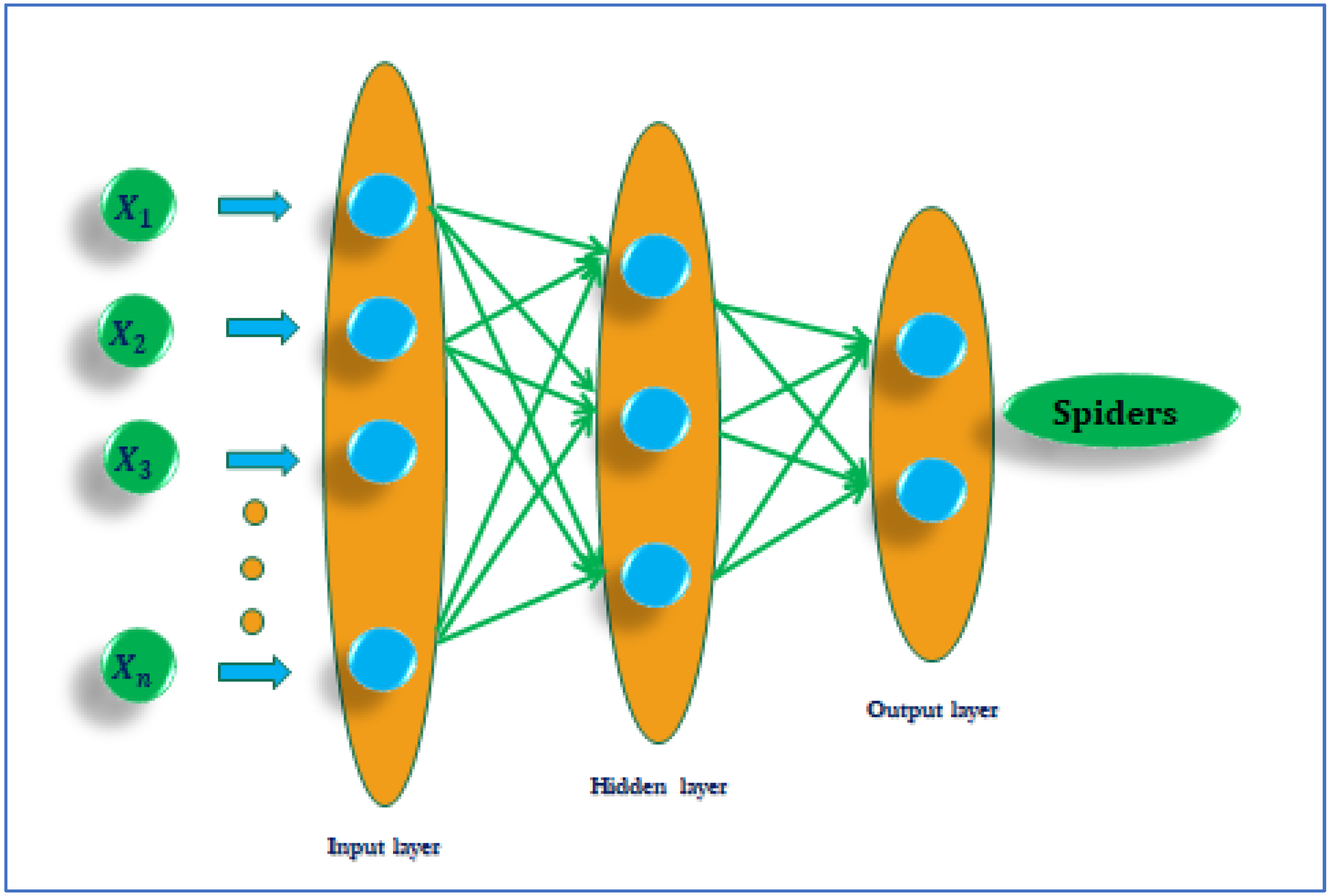
2.4. Artificial Neural Network (ANN)

ANNs are a type of nonlinear data-driven self-adaptive technique that can be used to model a variety of problems, particularly when the underlying data relationship is unknown. The adaptive nature of these networks, in which “learning by example” replaces “programming” in problem solving, is a key characteristic. The neural networks are made up of layers of neurons that are connected in such a way that one layer takes input from the previous layer and transfers the output to the next one. The multi-layer perceptron (MLP), a type of feed-forward neural network, is the most widely-used ANN. There are at least three levels of nodes in MLP. Each node, with the exception of the input nodes, is a neuron with a nonlinear activation function. For training, MLP employs a supervised learning approach. MLP is distinguished from a linear perceptron by its numerous layers and non-linear activation, which discriminate data that is not linearly separable. Figure 2 shows a graphical representation of MLP.

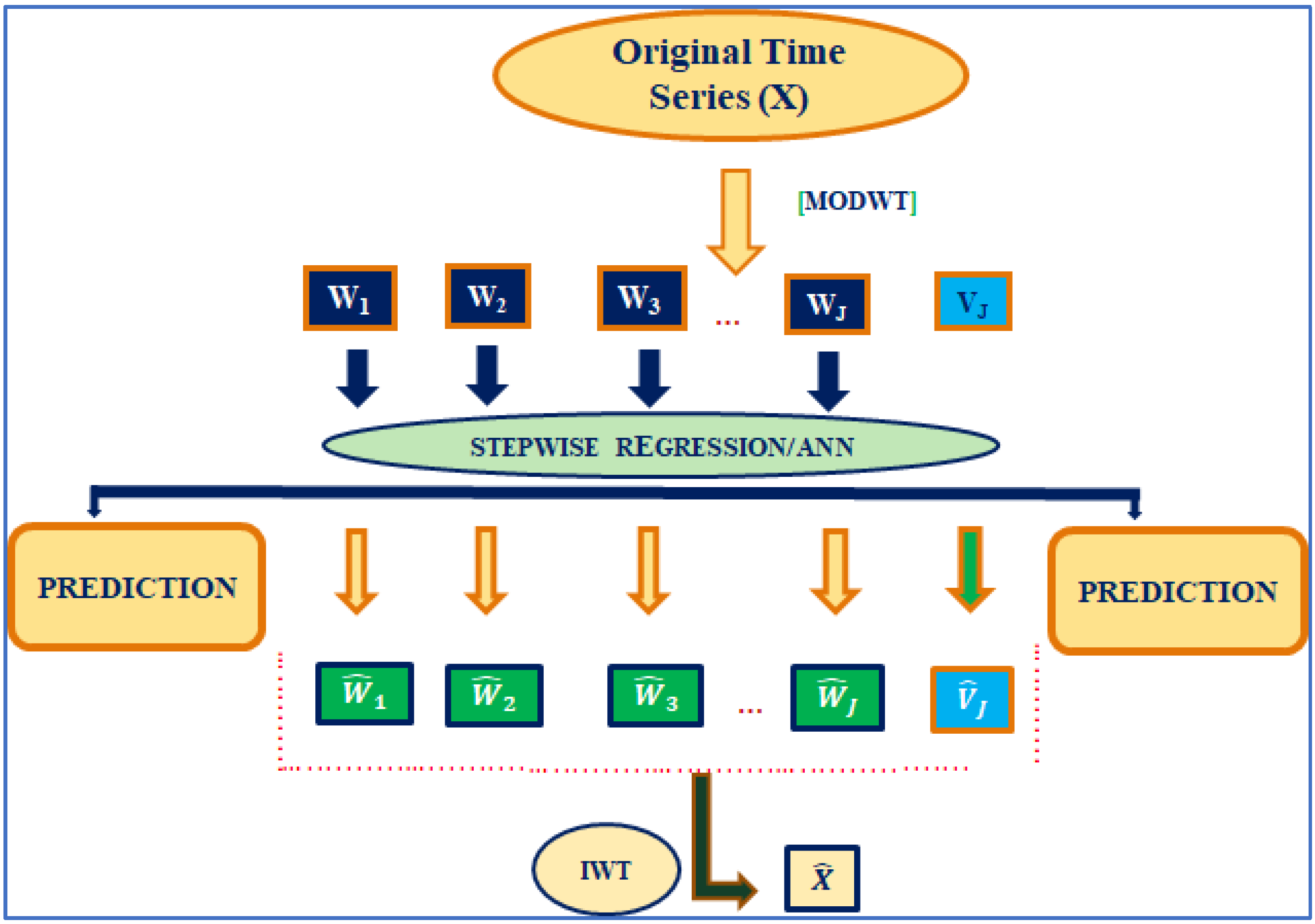
2.5. Wavelet–Linear Regression (W–LR) Approach

Wavelet decomposition followed by application of LR is carried out. In the first step, the original time-series is decomposed into a certain number of sub-series (W₁, W₂, …, W_J, V_J) by non-decimated wavelet transform (MODWT) using an appropriate level of decomposition. W₁, W₂, …, W_J are wavelet detail components, and V_J is a smooth component. These play different role in the original time series and the behavior of each sub-series is distinct from others.

In the second step, the stepwise selection technique is advocated to select the weather variables for developing regression model for each of the decomposed sub-series

Third step: prediction for each sub series is obtained by the model developed in the third step.

Fourth step: prediction of actual series is obtained by means of inverse wavelet transform.

2.6. Wavelet–ANN (W–ANN) Approach

The algorithm as proposed for W–LR approach will remain same for the W–ANN approach, except for the second step.

In the second step, instead of a stepwise regression model, ANN is applied for developing the model on each of the decomposed series. The key of the W–ANN hybrid model is wavelet decomposition of time series and the construction of ANN.

The schematic representation of W–LR and W–ANN algorithm is given in Figure 3. Figure 3 illustrates the procedure to obtain the forecasts employing wavelets and ANN. Multi-time scale and an observed highly nonlinear pattern in the transformed series led to application of ANN for prediction purposes. When the original series has much nonlinearity as its property, the MODWT simplifies it by breaking it into its sub-frequencies. Therefore, the ANN can now model the details and approximate components sufficiently so that the accuracy of the forecasting process is improved to a marked extent. Wavelet analysis can effectively diagnose a signal’s main frequency component and abstract local information of the time-series. For computation purposes, one R package, WaveletANN, has been developed and is available at https://CRAN.R-project.org/package=WaveletANN (accessed on 2 January 2022) [29].

2.7. Validation

Prior to analysis, the dataset was divided into two sets, i.e., an estimation set and validation set. Proportionally, 80% of the observations were used for estimation purpose and the remaining 20% of the observations were kept for validation. Comparative assessment of prediction performance of different models, namely LR, W–LR, and W–ANN, was carried out in terms of mean absolute percentage error (MAPE) by the following formula:

$$\mathrm{MAPE}=1/h{{\displaystyle \sum }}_{i=1}^h\left\{\left|y_{t+i}-{\widehat{y}}_{t+i}\right|/y_{t+i}\right\}\times 100$$

(1)

where h denotes the number of observations for validation, $y_i$ is the observed value, and ${\widehat{y}}_i$ is the predicted one. Diebold Mariano test [23] was also conducted for different pairs of models to test for the significant difference in predictive accuracy between two competing models.

3. Results and Discussion

3.1. Spiders of Pigeon Pea Ecosystem and Description of Study Locations

Each insect in a given agroecosystem usually has numerous natural enemies [30], which could also have enemies [31] along trophic levels. A plant affected by an insect might produce volatiles which attracts natural enemies of this particular insect [32,33,34,35], but the same chemicals may also attract more insects [36]. Spiders are efficient predators; their good searching ability, wide host range, adaptation, low metabolic rate, energy conservation mechanism, and polyphagous nature make them model predatory fauna of pigeon pea ecosystems. Three species, i.e., lynx spider (Oxyopus sp.), sac spider (Clubiona sp.), and orb weaver spider (Araneus sp.), predominantly predate the lepidopterous larvae of pigeon pea insects, viz., Lampides boeticus, Excelatis atomosa, and Grapholita critica. Two spider species, Lycosa sp. and Paradosa sp., are commonly reported at Gujarat. Considering that the species-wise record of spiders is cumbersome in the farms and that spiders are general predators in all ecosystems, the present investigation recorded mainly web-spinning and jumping categories of spiders together, at all study locations. Details of ACZ and agro-ecological region (AER) with geographical coordinates of each location, along with the duration of the pigeon-pea-growing period in terms of standard meteorological weeks (SMW), are furnished in

Table 1. Details of study locations.

Location	Agro-Ecological Region	Agro-Climate Zone	GPS Co-Ordinates	Study Period	Crop Season (SMW)
Anantapur	Deccan plateau and central highland, hot arid ecoregion	Southern Plateau and Hills Region	14°43′ N, 77°40′ E	2013–2016	30–52
SK Nagar	Western plain, Kachhh and part of Kathiawar peninsula, hot arid ecoregion	Gujarat Plains and Hills Region	21°10′ N, 72°51′ E	2011–2016	37–52
Gulbarga	Deccan plateau Aravallis, hot semi-arid ecoregion	Southern Plateau and Hills Region	17°21′ N, 76°48′ E	2012–2016	28–52
Jabalpur	Central highland (Malwa, Bundelkhand, and eastern Satpura), hot semi-humid ecoregion	Central Plateau and Hills Region	23°10′ N, 79°59′ E	2011,12,15 &16	26–51
Rahuri	Deccan plateau Aravallis, hot semi-arid ecoregion	Western Plateau and Hills Region	19°22′ N, 74°39′ E	2011–2013	31–52
Vamban	Eastern ghat, TN upland and decan plateau, hot semi-arid ecoregion	East Coast Plains and Hills Region	10°21′ N, 78°54′ E	2011–2017	30–52
Warangal	Decan plateau and eastern ghat, hot semi-arid ecoregion	Southern Plateau and Hills Region	18°00′ N, 79°36′ E	2011–2017	33–52

. The occurrence of spiders (spiders/plant) was considered as the response variable and the weather variables namely maximum temperature (MaxT), minimum temperature (MinT), relative humidity morning (RHM), relative humidity evening (RHE), sunshine (SS), rainfall (RF), no. of rainy days (RD), and wind speed (Wind) were the explanatory variables.

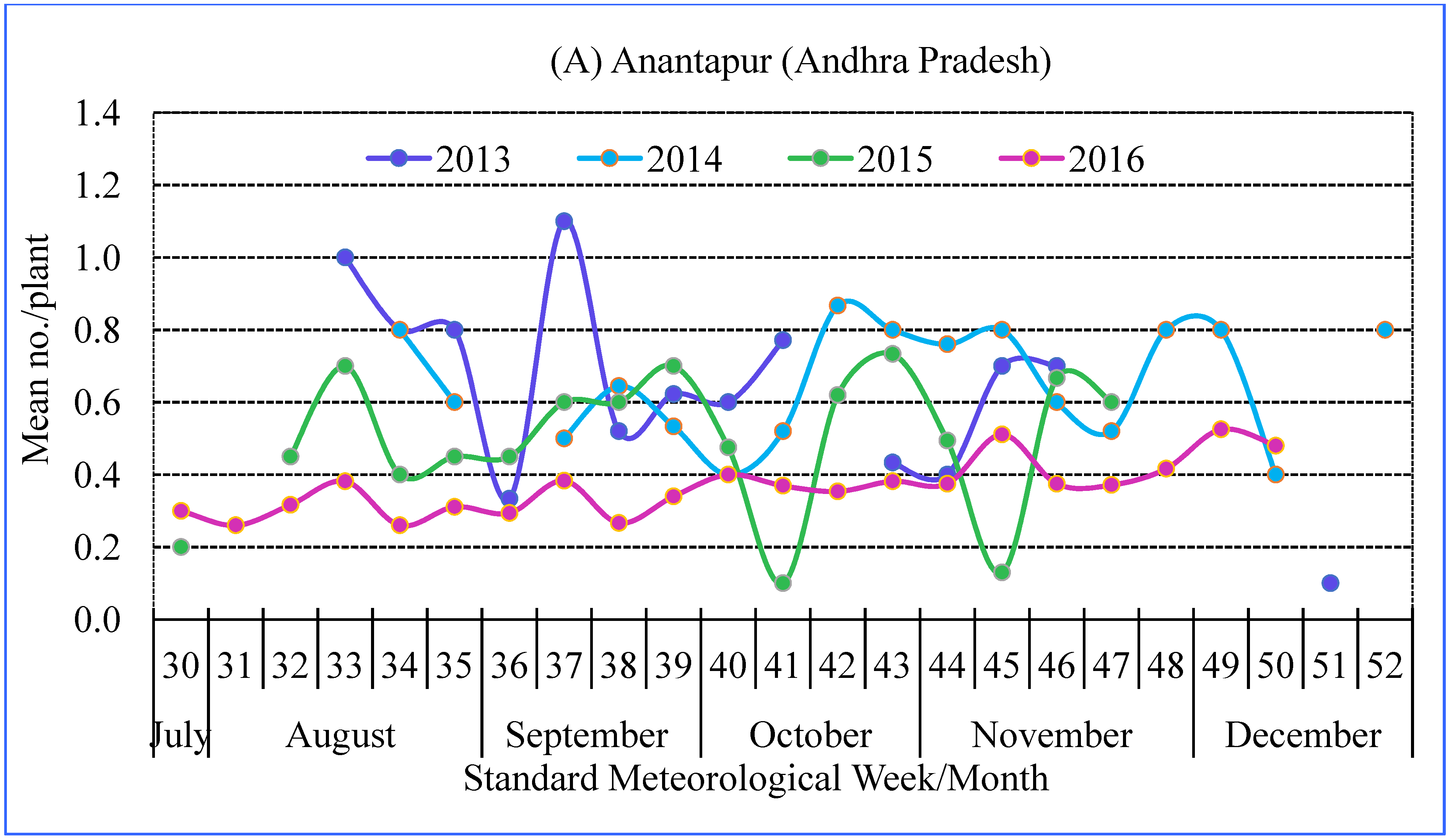
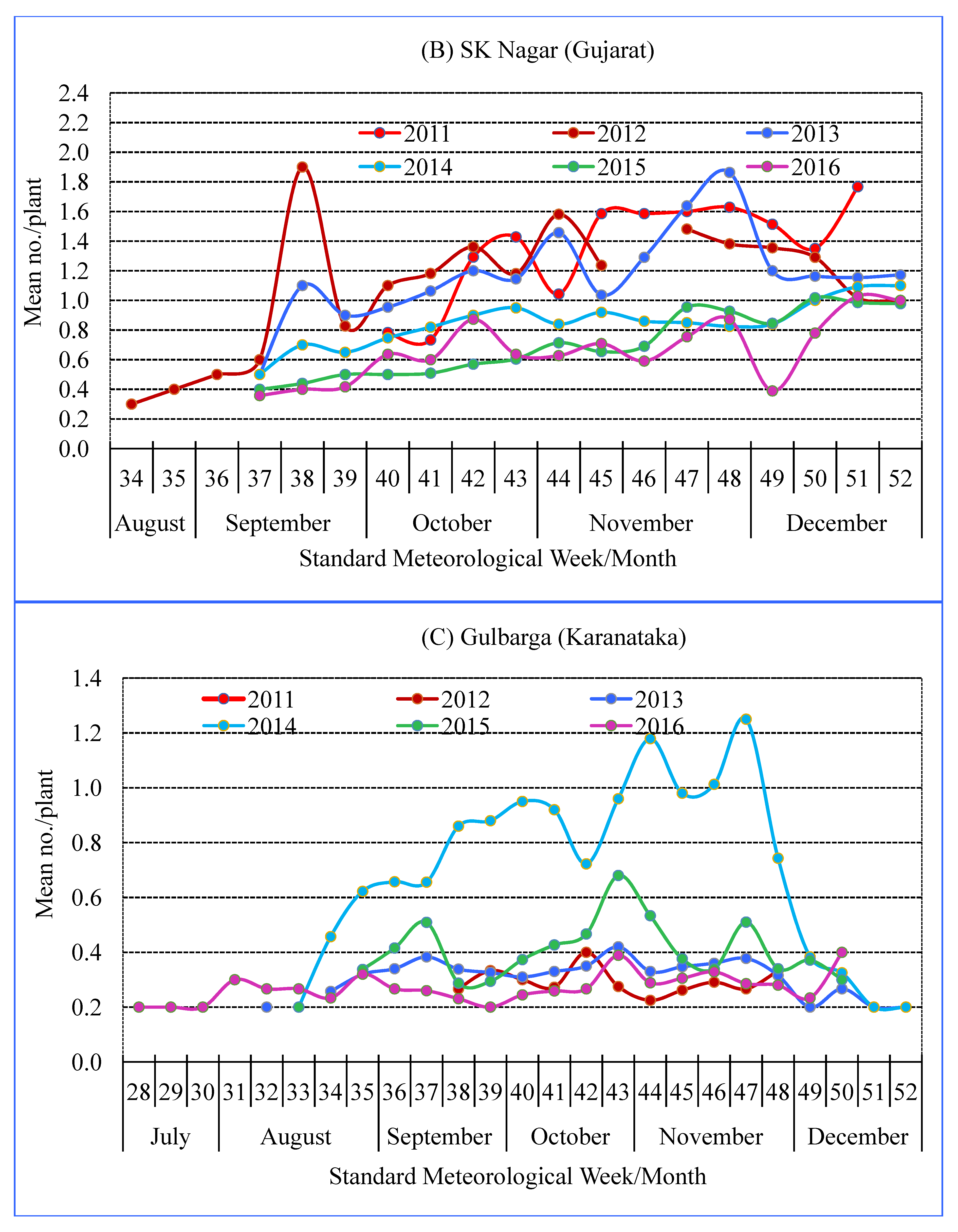
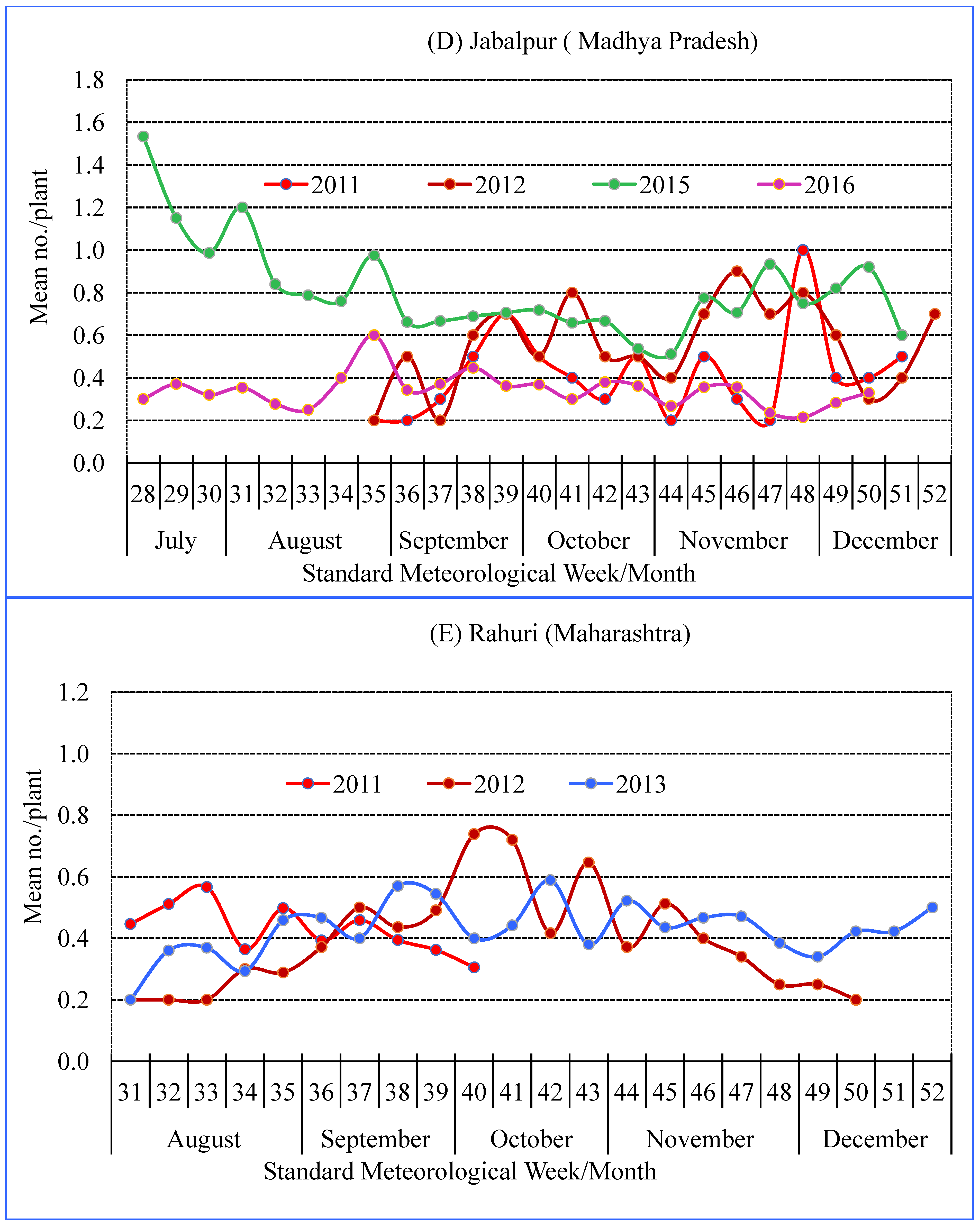
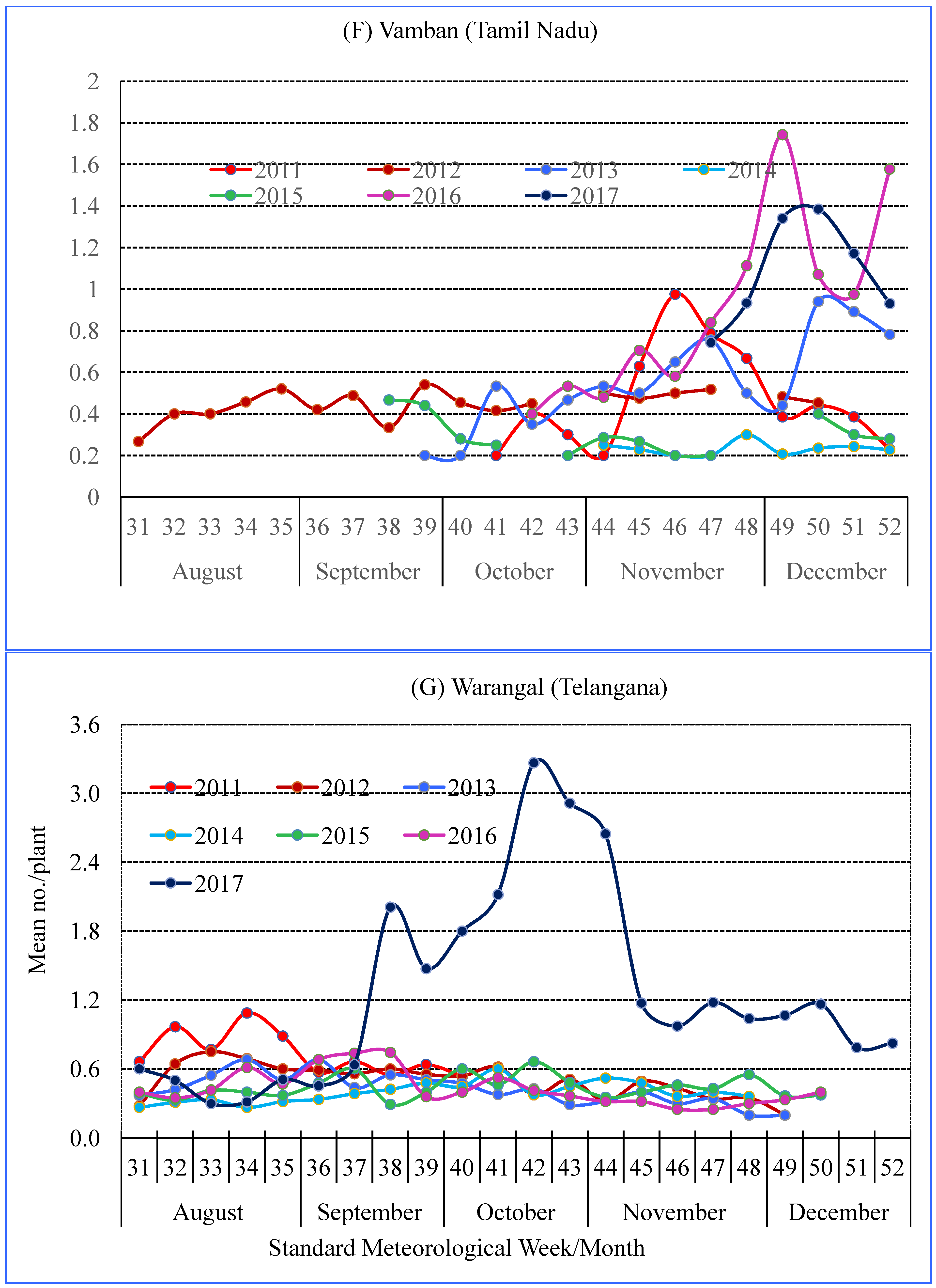
3.2. Seasonality of Spiders

The seasonal dynamics of spider populations are depicted in Figure 4A–G. The spider population at Anantapur remained low (<1) during 2013–2016, except 2013 when population (mean number/plant) crossed >1 at 37 SMW (Figure 4A). However, at SK Nagar, spider population remained high (>1) during 2011–2013, while during 2014–2016, the population was lower (Figure 4B); at Gulbarga, spider population crossed 1 during the crop period 2014, with the highest recorded during 47 SMW in 2014 (Figure 4C). At Jabalpur, spider population remained low (<1) during the crop period 2011–2016, except 2015, when the population crossed 1 (Figure 4D). In Rahuri, the population remained <1 during the entire crop season of 2011–2015 (Figure 4E). At Vamban, the spider population remained >1/plant during 2016–2017 (Figure 4F), and in Warangal, almost the whole crop season of 2017 (Figure 4G).

The general rule adopted for management decisions relying on the insect/pest and defender ratio is 2:1 [37]. Based on the criteria, all the seasons and time periods having a mean spider level of more than one/plant at each study location can be said to provide natural regulation of a single or multiple insects occurring on pigeon pea farms. Although it is beyond the scope of the current investigation to make associations with the insect spectrum at each of the locations, the varied abundance across seasons within a given location and across locations for a given season indicated the differing potential of spiders as predators, justifying the need for a good location-specific model for forecasting spiders.

3.3. Descriptive Statistics of Spider Occurrence

The descriptive statistics of spider occurrence have been reported in

Table 2. Descriptive statistics of response variable.

Statistical Measures	Spiders (Response Variable)
	Anantapur (AP)	SK Nagar (GJ)	Gulbarga (KA)	Jabalpur (MP)	Rahuri (MH)	Vamban (TN)	Warangal (TS)
Mean	0.76	0.89	0.50	0.74	0.50	0.63	0.77
Median	0.60	0.80	0.40	0.60	0.40	0.40	0.60
Maximum	5.40	5.20	5.40	5.60	6.00	7.00	10.20
Minimum	0.10	0.20	0.20	0.20	0.10	0.10	0.20
SD #	0.54	0.65	0.45	0.54	0.44	0.56	0.68
CV # (%)	71.64	73.69	89.95	73.10	87.83	88.42	88.90
Skewness	2.54	1.43	4.00	2.34	4.63	3.64	5.73
Kurtosis	12.17	2.84	4.00	10.70	38.48	25.35	59.45

# SD: standard deviation; CV: coefficient of variation.

. Table 2 indicates that, in all the locations, spiders showed positively skewed and leptokurtic distribution. Variability in spider population measured in terms of coefficient of variation (CV) was higher, ranging from 71.6% in Anantapur to 89.9% in Gulbarga over 2011–17. Maximum spider population varied from 5.2 (mean no./plant) in S K Nagar to 10.2 in Warangal, with minimum records of 0.1 to 0.2 at various locations during different time periods (Table 2).

Before further analysis, a normality check was carried out by means of Kolmogorov–Smirnov test and Anderson–Darling test; it was observed that the spider population in all the locations significantly deviated from normality (

Table 3. Goodness-of-Fit Tests for Normal Distribution.

Location	Kolmogorov–Smirnov		Anderson–Darling
	Statistic	p-Value	Statistic	p-Value
Anantapur	0.16	<0.010	33.05	<0.005
SK Nagar	0.16	<0.010	31.03	<0.005
Gulbarga	0.28	<0.010	82.83	<0.005
Jabalpur	0.17	<0.001	36.66	<0.005
Rahuri	0.24	<0.010	68.80	<0.005
Vamban	0.25	<0.010	63.76	<0.005
Warangal	0.20	<0.010	52.52	<0.005

) [38]. Non-normality of the data triggered a nonparametric method for modeling spider occurrence based on climatic variables.

3.4. Spider–Weather Relations

The range of weather variables across all studied locations have been reported in

Table 4. Range of weather variables during study seasons.

Location	MaxT (°C)	MinT (°C)	RHM (%)	RHE (%)	RF (mm)	SS (h/day)	Wind (km/h)	RD (No. of Days)
Anantapur	35.66–28.46	25.5–14.11	99–71.86	68.29–21.71	168.3–0	19.43–0.29	19.57–2	6–0
SK Nagar	38.84–25.21	27.14–4.94	95.25–8.9	89.43–18	383.6–0	10.14–10.43	14.1–0.38	5–0
Gulbarga	33.19–26.26	26.93–9.46	94.04–53.07	80.17–24.27	195–0	Not available	52.29–0	5–0
Jabalpur	35.1–23.36	24.54–4.18	9571–77.71	88.86–22	221.6–0	9.71–0	8.43–1.43	7–0
Rahuri	33.66–28.23	22.63–7.40	87.57–46.29	70.57–24.86	118.6–0	9.86–2.14	8.14–0.14	5–0
Vamban	38.36–27.00	25.86–16.20	96.25–72.43	92–59.86	256–0	8.29–0	6–0.71	6–0
Warangal	32.86–27.88	24.93–12.75	91.86–82	73.14–38.75	117.4–0	7.86–1	-	4–0

MaxT: maximum temperature; MinT: minimum temperature, RHM: relative humidity morning; RHE: relative humidity evening; SS: sunshine; RF: rainfall; RD: number of rainy days and Wind: wind speed.

. Correlation analysis (Pearson method) of spider occurrence with weather variables lagged by one week (

Table 5. Correlation coefficients between spiders with weather factors, lagged by one week ^# (aggregate years).

Weather Parameters	Anantapur	SK Nagar	Gulbarga	Jabalpur	Rahuri	Vamban	Warangal
MaxT-1	−0.11 *	−0.11 ***	0.12 ***	0.15 ***	0.01	−0.14 ***	0.29 ***
MinT-1	−0.18 ***	−0.28 ***	0.20 ***	0.19 ***	0.09 *	0.10 **	0.15 ***
RHM-1	−0.09 *	−0.05 *	−0.04	−0.19 **	0.10 **	−0.05	0.07 **
RHE-1	−0.001	−0.35 ***	−0.10 **	0.12 **	0.08 *	0.13 ***	−0.01
RF-1	−0.01	−0.03	−0.04	0.07 *	0.16 ***	−0.09 **	−0.001
SS-1	−0.33 ***	0.22 ***	−	−0.09 *	−0.03	0.12 **	−0.13 ***
Wind-1	−0.06	0.02	0.28 ***	0.19 ***	−0.09 *	−0.08 *	−
RD-1	−0.03	−0.08 **	0.06 *	0.08 *	0.17 ***	0.001	0.005

^# The suffix 1 denotes the lag in weeks of weather relating to spider occurrence considered for correlations. ***: significant at p < 0.001; **: significant at p < 0.01; *: significant at p < 0.05.

) on data sets aggregated over the study seasons of each location indicated significant and negative influence of MaxT, MinT, RHM, and SS at Anantapur. Elevated temperature basically favors adult hunting insects and spiders, and it seems that the lethal temperature of many spiders is much above the temperature expected by climate change [39], a positive attribute from the ecological perspective. For S K Nagar, all the weather variables under consideration except RF and Wind were found to be significant with the occurrence of spiders; amongst them, only SS had positive influence while all other variables had negative influence. At Gulbarga, RHE had significant negative correlation with spider occurrence, whereas MaxT, MinT, Wind, and RD all had positive influence. All the weather variables were found to be positively significant, except RHM and SS, in determining occurrence of spiders at Jabalpur; RHM and SS have negative influence in this location. At Rahuri, Wind was negatively correlated with spider occurrence whereas, MinT, RHM, RHE, RF, and RD had positive influence. MaxT, RF, and Wind had negative association, while MinT, RHE, and SS had positive association with spider occurrence at Vamban. At Warangal, MaxT, MinT, and RHM have positive correlation, whereas SS has negative correlation with the occurrence of spiders.

3.5. Modeling of Spiders

A stepwise LR model was applied for forecasting spider occurrence at each of the seven respective locations based on eight weather variables. The final equations of the LR models are specified in

Table 6. Stepwise regression models for prediction of spiders.

Location	Model Equation
Anantapur	1.09 2212 0.014 MaxT-1 − 0.009 SS-1
SK Nagar	1.64 − 0.014 MaxT-1 − 0.005 RHE-1 + 0.005 RF-1 + 0.03 RD-1 + 0.004 SS-1 + 0.05 Wind-1
Gulbarga	0.21 + 0.01 MaxT-1 + 0.003 MinT-1 + 0.01 RF-1 + 0.005 Wind-1
Jabalpur	1.65 + 0.01 MinT-1 − 0.007 RHM-1 − 0.003 RHE-1 − 0.0003 RF-1 − 0.01 SS-1 + 0.02 Wind-1
Rahuri	0.91 + 0.002 MinT-1 + 0.01 RD-1 − 0.01 Wind-1
Vamban	1.20 − 0.02 MaxT-1 + 0.02 MinT-1 − 0.01 RD-1 + 0.01 SS-1
Warangal	−0.38 + 0.04 MaxT-1 +0.008 RHM-1 − 0.001 RHE-1 − 0.06 RD-1 − 0.05SS-1

. The climatic variables appeared in the equation were all significant at 5% level of significance.

Time series data on spider occurrence were decomposed by Haar wavelet filter. The maximum level of possible decomposition was taken as $J_0\le { \log }_2\left(N\right)$ in the present study, while the level of decomposition chosen was 5 in order to visualize the local as well as global pattern in the spider occurrence for Anantapur. A total of six series, namely W1, W2, W3, W4, W5, and V5 were generated. Similarly, at SK Nagar, Gulbarga, Jabalpur, and Warangal, the level of decomposition chosen was 7 and therefore, a total of eight series, namely W1, W2, W3, W4, W5, W6, W7, and V7, were generated. The level of decomposition chosen was 6 in Rahuri and Vamban, thus generating a total of seven series, namely W1, W2, W3, W4, W5, W6, and V6. The pattern of decomposition for each location is presented in Figure 5.

As discussed in the methodology section, a stepwise regression model was applied to predict individual components of the decomposed series. Similarly, for the W–ANN model, ANN was applied on each of the decomposed series. The best architecture selected for individual series in terms of no. of input lags and hidden nodes based on minimum mean square error are reported in

Table 7. Selection of W–ANN model based on RMSE.

Location	W1		W2		W3		W4		W5		V
	# L	# HN	# L	# HN	# L	# HN	# L	# HN	# L	# HN	# L	# HN
Anantapur	1	1	1	1	1	1	4	2	4	2	6	3
SK Nagar	1	1	1	1	1	1	3	4	3	4	1	1
Gulbarga	1	1	1	1	1	1	1	1	1	1	1	1
Jabalpur	1	1	2	1	2	1	1	1	1	1	1	1
Rahuri	1	1	1	1	1	1	1	1	1	1	1	1
Vamban	1	1	1	1	2	1	4	1	4	1	1	1
Warangal	1	1	1	1	1	1	1	1	1	1	1	1

^# L: no. of lags; ^# HN: no. of hidden nodes.

.

3.6. Validation

After estimation of the models, forecasts were obtained for the validation data set. The performance of predictions of spider occurrence in pigeon pea through various models, viz., regression (LR), ANN, wavelet–regression and wavelet–ANN, were tested using RMSE and MAPE (

Table 8. RMSE values in relation to Linear Regression (LR), Wavelet–Linear Regression (W–LR) and Wavelet–ANN (W–ANN) models predicting of spiders.

Location	No. of Observations Used for		RMSE				MAPE (%)
	Estimation	Validation	LR	ANN	W–LR	W–ANN	LR	ANN	W–LR	W–ANN
Anantapur	363	40	0.079	0.801	0.079	0.064	9.3	9.2	9.1	8.0
SK Nagar	1427	159	0.117	0.113	0.106	0.104	8.6	8.5	8.5	7.3
Gulbarga	981	109	0.112	0.110	0.108	0.065	11.2	11.0	10.5	6.4
Jabalpur	659	73	0.147	0.143	0.141	0.134	8.5	8.2	8.1	6.3
Rahuri	545	61	0.138	0.135	0.133	0.105	11.3	11.1	11.0	7.4
Vamban	690	77	0.391	0.386	0.381	0.185	20.8	20.3	19.8	10.1
Warangal	1600	178	0.666	0.664	0.663	0.625	31.1	31.0	30.9	27.5

). Both the RMSE and MAPE values of wavelet–ANN model are less in comparison to other competing models. LR had the largest RMSE and MAPE over other models and hence distantly precise over all other models. The accuracy of prediction is in the order of W–ANN > W–LR > ANN > LR. Since wavelet and ANN are nonparametric in nature and could model the non-normal variates more precisely, the model captured the nonlinearity present in the dataset of spiders. Residuals diagnostics carried out for testing the adequacy of fitted models revealed that there were no autocorrelations.

Further, Diebold-Mariano test [34] was applied to compare forecasting performance among W–LR, W–ANN, ANN and LR models. The null hypothesis for the test was set as: the predictive accuracy of any two competing models is equal. Different combinations of comparison, their specific alternative hypothesis along with test statistics and their significance are reported in

Table 9. Testing predictive accuracy by D–M test.

Combinations	Alternative Hypothesis	D-M Statistic	p-Value
Anantapur
ANN and LR	Predictive accuracy of LR is less than that of ANN	0.70	0.76
W–LR and LR	Predictive accuracy of LR is less than that of W–LR	6.64	>0.99
W–LR and ANN	Predictive accuracy of ANN is less than that of W–LR	7.02	>0.99
W–ANN and LR	Predictive accuracy of LR is less than that of W–ANN	0.33	0.63
W–ANN and ANN	Predictive accuracy of ANN is less than that of W–ANN	−0.64	0.26
W–ANN and W–LR	Predictive accuracy of W–LR is less than that of W–ANN	−6.62	<0.0001
SK Nagar
ANN and LR	Predictive accuracy of LR is less than that of ANN	−1.70	0.05
W–LR and LR	Predictive accuracy of LR is less than that of W–LR	−1.72	0.04
W–LR and ANN	Predictive accuracy of ANN is less than that of W–LR	1.63	0.95
W–ANN and LR	Predictive accuracy of LR is less than that of W–ANN	−2.02	0.02
W–ANN and ANN	Predictive accuracy of ANN is less than that of W–ANN	−1.72	0.04
W–ANN and W–LR	Predictive accuracy of W–LR is less than that of W–ANN	−1.89	0.02
Gulbarga
ANN and LR	Predictive accuracy of LR is less than that of ANN	4.60	>0.99
W–LR and LR	Predictive accuracy of LR is less than that of W–LR	3.44	0.99
W–LR and ANN	Predictive accuracy of ANN is less than that of W–LR	5.17	>0.99
W–ANN and LR	Predictive accuracy of LR is less than that of W–ANN	−5.89	<0.0001
W–ANN and ANN	Predictive accuracy of ANN is less than that of W–ANN	−4.92	<0.0001
W–ANN and W–LR	Predictive accuracy of W–LR is less than that of W–ANN	−5.97	<0.0001
Jabalpur
ANN and LR	Predictive accuracy of LR is less than that of ANN	−1.94	0.03
W–LR and LR	Predictive accuracy of LR is less than that of W–LR	−2.03	0.02
W–LR and ANN	Predictive accuracy of ANN is less than that of W–LR	1.72	0.96
W–ANN and LR	Predictive accuracy of LR is less than that of W–ANN	−1.59	0.05
W–ANN and ANN	Predictive accuracy of ANN is less than that of W–ANN	1.55	0.94
W–ANN and W–LR	Predictive accuracy of W–LR is less than that of W–ANN	−0.96	0.16
Rahuri
ANN and LR	Predictive accuracy of LR is less than that of ANN	−0.30	0.38
W–LR and LR	Predictive accuracy of LR is less than that of W–LR	0.004	0.50
W–LR and ANN	Predictive accuracy of ANN is less than that of W–LR	0.28	0.61
W–ANN and LR	Predictive accuracy of LR is less than that of W–ANN	−4.93	<0.0001
W–ANN and ANN	Predictive accuracy of ANN is less than that of W–ANN	−1.78	0.04
W–ANN and W–LR	Predictive accuracy of W–LR is less than that of W–ANN	−6.99	<0.0001
Vamban
ANN and LR	Predictive accuracy of LR is less than that of ANN	−9.59	<0.0001
W–LR and LR	Predictive accuracy of LR is less than that of W–LR	−7.38	<0.0001
W–LR and ANN	Predictive accuracy of ANN is less than that of W–LR	9.36	>0.99
W–ANN and LR	Predictive accuracy of LR is less than that of W–ANN	−6.48	<0.0001
W–ANN and ANN	Predictive accuracy of ANN is less than that of W–ANN	−4.91	<0.0001
W–ANN and W–LR	Predictive accuracy of W–LR is less than that of W–ANN	−6.35	<0.0001
Warangal
ANN and LR	Predictive accuracy of LR is less than that of ANN	10.93	>0.99
W–LR and LR	Predictive accuracy of LR is less than that of W–LR	−5.07	<0.0001
W–LR and ANN	Predictive accuracy of ANN is less than that of W–LR	−11.92	<0.0001
W–ANN and LR	Predictive accuracy of LR is less than that of W–ANN	−13.07	<0.0001
W–ANN and ANN	Predictive accuracy of ANN is less than that of W–ANN	−17.56	<0.0001
W–ANN and W–LR	Predictive accuracy of W–LR is less than that of W–ANN	−12.97	<0.0001

. It was observed that, in Anantapur, the predictive accuracy of W–LR was lesser than W–ANN model whereas in other comparisons i.e., ANN vs. LR W–LR vs. LR, W–LR vs. ANN, W–ANN vs. ANN and W–ANN vs. LR, the test was not significant, implying absence of statistically significant differences in predictive accuracy in the pair of comparisons. In SK Nagar, Gulbarga, Jabalpur, Rahuri, Vamban, and Warangal, the model accuracy was of the following order: W–ANN > W–LR = ANN > LR, W–ANN > W–LR = ANN = LR, W–ANN = W–LR = ANN > LR, W–ANN > W–LR = ANN = LR, W–ANN > W–LR = ANN > LR, and W–ANN > W–LR > ANN = LR, respectively.

4. Conclusions

The decomposition approach of wavelet analysis coupled with machine learning techniques, viz., ANN and multiple regression models (LR), applied for modeling and forecasting the occurrence of spiders for different pigeon pea growing locations was the first of its kind in India. Wavelet decomposition carried out based on MODWT using Haar filter and levels of decomposition chosen based on the number of observations gave better results. The supremacy of W–ANN model on the basis of RMSE, MAPE, and Diebold-Mariano test was inferred. From the applied perspective, implementation of the spider forecasts using W–ANN model, at least in pigeon pea growing locations possessing a higher population (>1) for most periods of the growing season and many seasons, would be of immense use in the context of changing climate. More focus on propelling conservation biological control built around spiders would reduce insecticide use on pigeon pea, resulting in a residue-free commodity offering a safe and secure food system. Application of a similar approach to other candidate species (insects as well as diseases) of pigeon pea and in different crops stands out as an action point of recommendation in the area of plant protection.

References

1. Food and Agriculture Organization, Statistical Database 2003. Available online: https://www.fao.org/documents/card/en/c/19d2a310-cee0-5bfd-bdfe-3b3e64e789ed/ (accessed on 24 January 2022).
2. Food and Agriculture Organization. statistical database 2014. Mushrooms and Truffles. Rome: Food and Agriculture Organization of the United Nations. Available online: http://faostat3.fao.org/ (accessed on 1 August 2014).
3. Reddy, M.V.; Nene, Y.L. Estimation of yield loss in Pigeon pea due to sterility mosaic. In Proceedings of the International Workshop on Pigeon Pea, Patancheru, AP, India, 15–19 December 1980; The International Crops Research Institute for the Semi-Arid Tropics Center: Patancheru, India; pp. 305–312. [Google Scholar]
4. Laxman, S. Production as-pects of Pigeon pea and future prospects. In Uses of Tropical Grain Legumes, Proceedings of the Consultants Meeting, Patancheru, India, 27–30 March 1989; Laxman, S., Silim, S.N., Ariyanayagam, R.P., Reddy, M.V., Eds.; The International Crops Research Institute for the Semi-Arid Tropics Center: Patancheru, India, 1991; pp. 27–121. [Google Scholar]
5. Kannaiyan, J.; Nene, Y.L.; Reddy, M.V.; Ryan, J.G.; Raju, T.N. Prevalence of Pigeon pea disease and associated crop losses in Asia, Africa and the Americas. Tropical. Pest Manag. 1984, 30, 62–71. [Google Scholar] [CrossRef] [Green Version]
6. Ganapathy, K.N.; Gnanesh, B.N.; Gowda, B.M.; Venkatesha, S.C.; Gomashe, S.S.; Channamallikarjuna, V. AFLP analysis in Pigeon pea (Cajanus cajan (L.) Mill sp.) revealed close relationship of cultivated genotypes with some of its wild relatives. Genet. Resour. Crop Evol. 2011, 58, 837–847. [Google Scholar] [CrossRef]
7. Varshney, R.K.; Penmetsa, R.V.; Dutta, S.; Kulwal, P.L.; Saxena, R.K.; Datta, S.; Sharma, T.R.; Rosen, B.N.; Carrasquilla-Garcia, N.; Farmer, A.D.; et al. Pigeon pea genomics initiative (PGI): An international effort to improve crop productivity of Pigeon pea (Cajanus cajan L.). Mol. Breed. 2010, 26, 393. [Google Scholar] [CrossRef] [Green Version]
8. Srilaxmi, K.; Paul, R. Diversity of insect pests of Pigeon pea [Cajanus cajan (L.) Millsp.] and their succession in relation to crop phenology in Gulbarga, Karnataka. Ecoscan 2010, 4, 273–276. [Google Scholar]
9. Shanower, T.G.; Romeis, J.E.; Minja, M. Insect Pests of Pigeon pea and Their Management. Annu. Rev. Entomol. 1999, 44, 77–96. [Google Scholar] [CrossRef] [Green Version]
10. Ghosh, S.K.; Kada, R.; Subbiah, J.; Ahsan, C.R.; Bari, L.; Mai, D.S.; Suong, N.K. Asian Food Safety and Security Association, Dhaka, Bangladesh. In Proceedings of the 2nd AFSSA Conference on Food Safety and Food Security, Dong Nai University of Technology, Bien Hoa, Vietnam, 15–18 August 2014; pp. 66–71. [Google Scholar]
11. Patel, M.L.; Patel, K.G.; Pandya, H.V. Navbharath Enterprises, Bangalore, India. Insect Environ. 2005, 11, 23–25. [Google Scholar]
12. Box, G.E.P.; Jenkins, G. Time Series Analysis, Forecasting and Control; Holden-Day: San Francisco, CA, USA, 1970. [Google Scholar]
13. Paul, R.K.; Das, M.K. Statistical modelling of inland fish production in India. J. Inland Fish. Soc. India 2010, 42, 1–7. [Google Scholar]
14. Paul, R.K.; Prajneshu, G.H. Wavelet frequency domain approach for modelling and forecasting of Indian monsoon rainfall time-series data. J. Indian Soc. Agric. Stat. 2013, 67, 319–327. [Google Scholar]
15. Paul, R.K.; Alam, W.; Paul, A.K. Prospects of livestock and dairy production in India under time series framework. Indian J. Anim. Sci. 2014, 84, 130–134. [Google Scholar]
16. Paul, R.K.; Ghosh, H.; Prajneshu. Development of out-of-sample forecast formulae for ARIMAX-GARCH model and their application. J. Indian Soc. Agric. Stat. 2014, 68, 85–92. [Google Scholar]
17. Arya, P.; Paul, R.K.; Kumar, A.; Singh, K.; Sivaramne, N.; Chaudhary, P. Predicting pest population using weather variables: An ARIMAX time series framework. Int. J. Agric. Stat. Sci. 2015, 11, 381–386. [Google Scholar]
18. Kim, Y.; Yoo, S.; Gu, Y.; Lim, J.; Han, D.; Baik, S. Crop pests prediction method using Regression and machine learning technology: Survey. IERI Procedia 2014, 6, 52–56. [Google Scholar] [CrossRef] [Green Version]
19. Paul, R.K.; Vennila, S.; Yadav, S.K.; Bhat, M.N.; Kumar, M.; Chandra, P.; Paul, A.K.; Prabhakar, M. Weather based Forecasting of Sterility Mosaic Disease in Pigeon pea using Machine Learning Techniques and Hybrid Models. Indian J. Agric. Sci. 2020, 90, 1952–1958. [Google Scholar]
20. Paul, R.K.; Vennila, S.; Bhat, M.N.; Yadav, S.K.; Sharma, V.K.; Nisar, S.; Panwar, S. Prediction of early blight severity in tomato (Solanum lycopersicum) by machine learning technique. Indian J. Agric. Sci. 2019, 89, 169–175. [Google Scholar]
21. Paul, R.K.; Garai, S. Performance comparison of wavelets-based machine learning technique for forecasting agricultural commodity prices. Soft Comput. 2021, 25, 12857–12873. [Google Scholar] [CrossRef]
22. Paul, R.K.; Paul, A.K.; Bhar, L.M. Wavelet-based combination approach for modeling sub-divisional rainfall in India. Theor. Appl. Climatol. 2020, 139, 949–963. [Google Scholar] [CrossRef]
23. Calvo, L.; Guzmán, M.; Guzmán, J. Considerations about Application of Machine Learning to the Prediction of Sigatoka Disease. In Proceedings of the World Conference on Computers in Agriculture and Natural Resources, University of Costa Rica, San Jose, Costa Rica, 27–30 July 2014; Available online: http://CIGRProceedings.org (accessed on 10 January 2022).
24. Diebold, F.X.; Mariano, R.S. Comparing predictive accuracy. J. Bus. Econ. Stat. 1995, 13, 253–263. [Google Scholar]
25. Chatterjee, S.; Hadi, A.S. Sensitivity Analysis in Linear Regression; John Wiley and Sons, Inc.: New York, NY, USA, 1988. [Google Scholar]
26. Daubechies, I. Ten Lectures on Wavelets; SIAM: Philadelphia, PA, USA.
27. Percival, D.B.; Walden, A.T. Wavelet Methods for Time-Series Analysis; Cambridge University Press: Cambridge, UK, 2000. [Google Scholar]
28. Ogden, T. Essential Wavelets for Statistical Applications and Data Analysis; Birkhauser: Boston, MA, USA, 1997. [Google Scholar]
29. Paul, R.K. WaveletANN: Wavelet ANN Model. R Package Version 0.1.0. 2019. Available online: https://CRAN.R-project.org/package=WaveletANN (accessed on 2 January 2022).
30. Hunter, M.D. Trophic promiscuity, intraguild predation and the problem of omnivores. Agric. For. Entomol. 2009, 11, 125–131. [Google Scholar] [CrossRef]
31. CPC. Crop Protection Compendium. CAB International. 2009. Available online: http://www.cabi.org/compendia/cpc/ (accessed on 4 January 2022).
32. Takabayashi, J.; Sabelis, W.M.; Janssen, A.; Shiojiri, K.; van Wijk, M. Can plants betray the presence of multiple herbivore species to predators and parasitoids? The role of learning in phytochemical information networks. Ecol. Res. 2006, 21, 3–8. [Google Scholar] [CrossRef] [Green Version]
33. Khan, Z.R.; James, D.G.; Midega, C.A.O.; Pickett, J.A. Chemical ecology and conservation biological control. Biol. Control. 2008, 45, 210–224. [Google Scholar] [CrossRef]
34. Schnee, C.; Köllner, T.G.; Held, M.; Turlings, T.C.J.; Gershenzon, J.; Degenhardt, J. The products of a single maize sesquiterpene synthase form a volatile defense signal that attracts natural enemies of maize herbivores. Proc. Natl. Acad. Sci. USA 2013, 103, 1129–1134. [Google Scholar] [CrossRef] [Green Version]
35. Degenhardt, J. Indirect Defense Responses to Herbivory in Grasses. Plant Physiol. 2009, 149, 96–102. [Google Scholar] [CrossRef] [Green Version]
36. Unsicker, S.B.; Kunert, G.; Gershenzon, J. Protective perfumes: The role of vegetative volatiles in plant defense against herbivores. Curr. Opin. Plant Biol. 2009, 12, 479–485. [Google Scholar] [CrossRef]
37. Satyagopal, K.; Sushil, S.N.; Jeyakumar, P.; Shankar, G.; Sharma, O.P.; Boina, D.R.; Sain, S.K.; Lavanya, N.; Sunanda, B.S.; Ram, A.; et al. AESA Based IPM Package for Redgram; Directorate of Plant Protection: Faridabad, India, 2014; p. 42.
38. Anderson, T.W.; Darling, D.A. Asymptotic theory of certain “goodness of fit” criteria based on stochastic processes. Ann. Math. Stat. 1952, 23, 193–212. [Google Scholar] [CrossRef]
39. Hanna, C.J.; Cobb, V.A. Critical Thermal Maximum of the Green Lynx Spider, Peucetia viridans (Araneae, Oxyopidae). J. Arachnol. 2007, 35, 193–196. [Google Scholar] [CrossRef]
Figure 1. Study locations.
Agronomy 12 01429 g001
Figure 2. A multilayer perceptron (MLP) architecture with one hidden layer.
Agronomy 12 01429 g002
Figure 3. Schematic representation of W–LR and W–ANN algorithm (MODWT: Maximal overlap discrete wavelet transform; IWT: Inverse wavelet transform).
Agronomy 12 01429 g003
Figure 4. (AG): Seasonal variation of spider occurrence.
Agronomy 12 01429 g004aAgronomy 12 01429 g004bAgronomy 12 01429 g004cAgronomy 12 01429 g004d
Figure 5. Maximal overlap discrete wavelet transform (MODWT) of spider occurrence across the locations.
Agronomy 12 01429 g005aAgronomy 12 01429 g005b