
Digital Mapping of Soil Organic Matter and Cation Exchange Capacity in a Low Relief Landscape Using LiDAR Data

 ,
,  and
and 
Abstract
:- In a low relief environment, SOM and CEC variation were captured using lidar elevation data
- Universal kriging, random forest, and cubits predictive models performed similarly
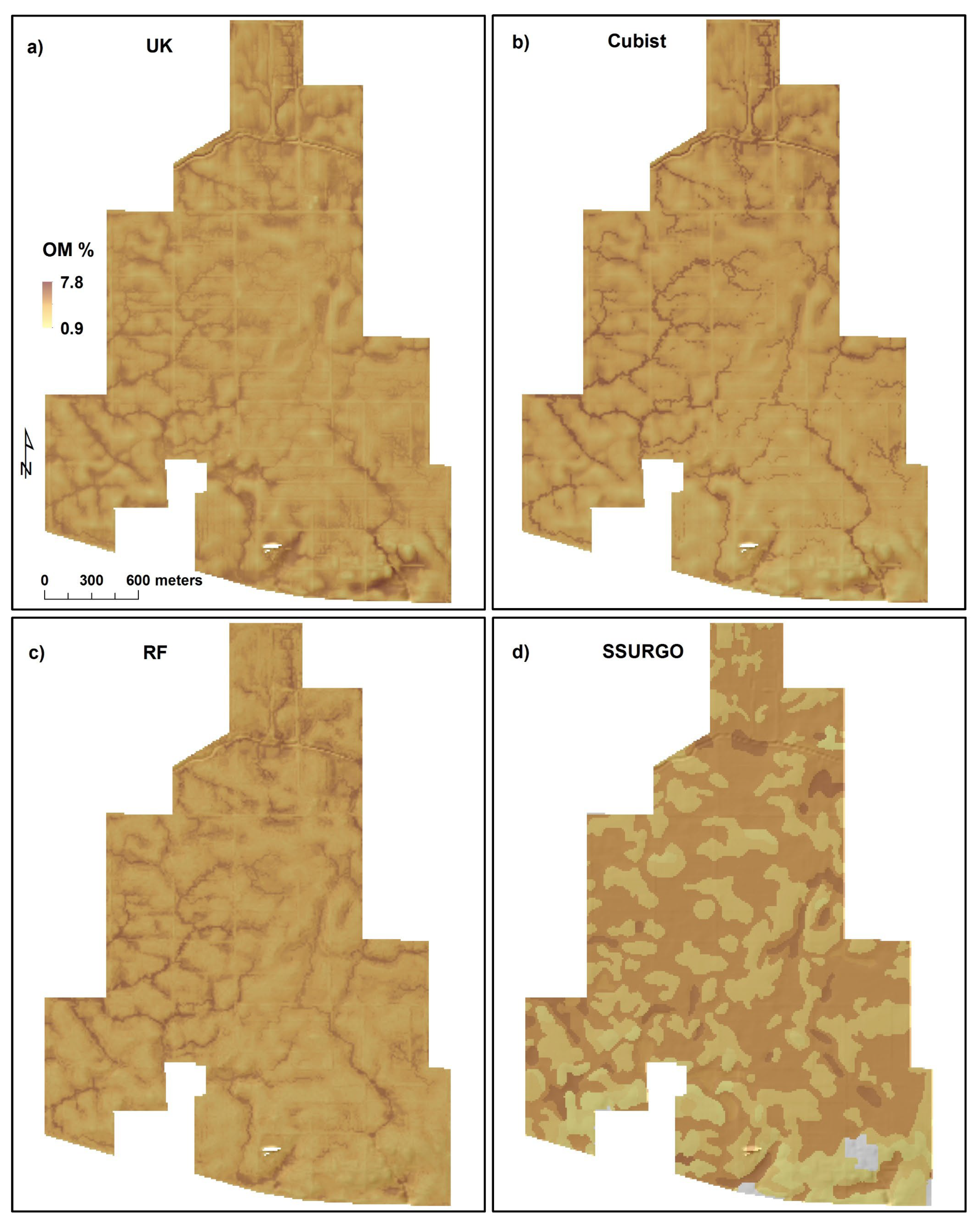
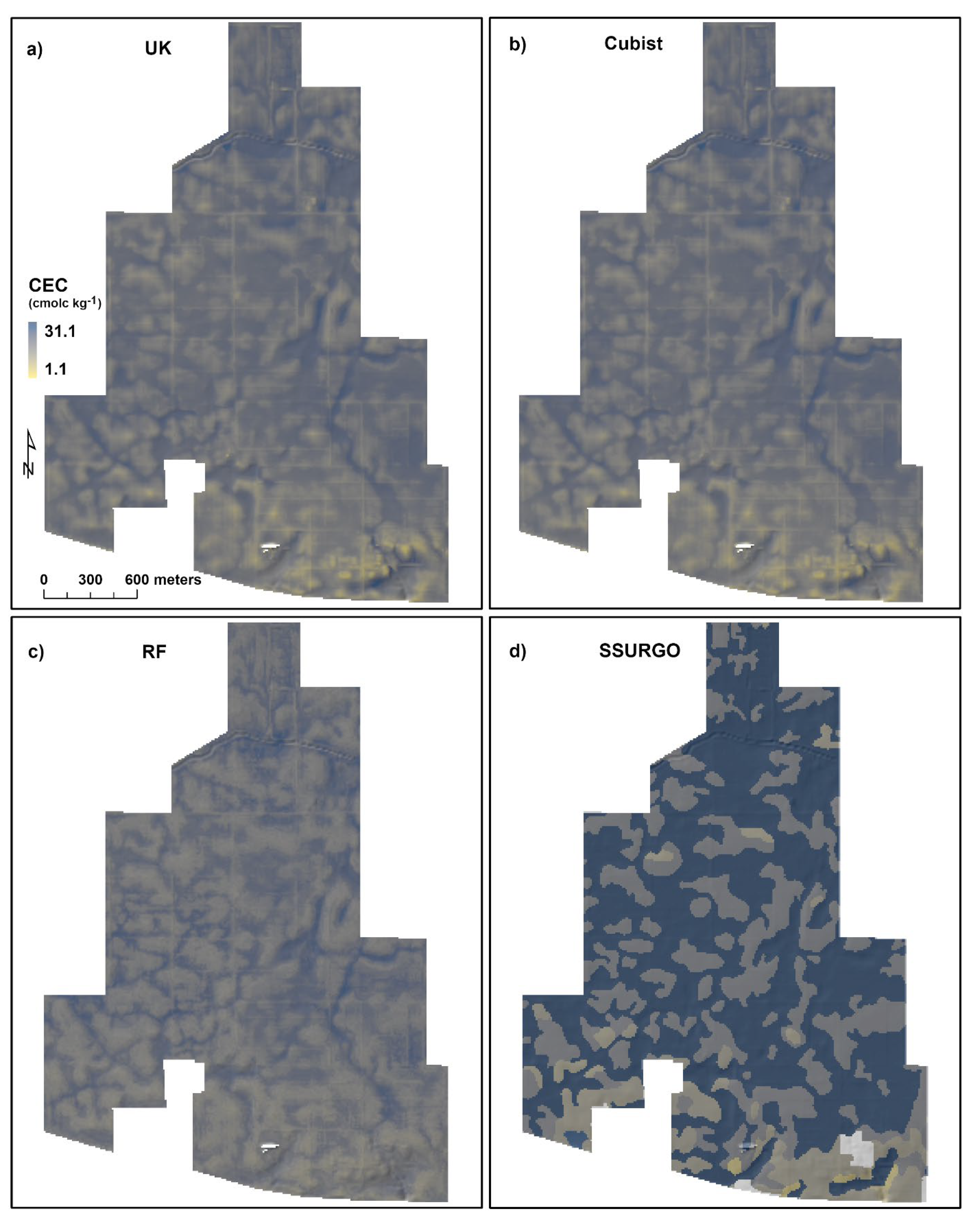
- Predictive models provided more detailed spatial distribution of SOM and CEC compared to SSURGO
1. Introduction
2. Materials and Methods
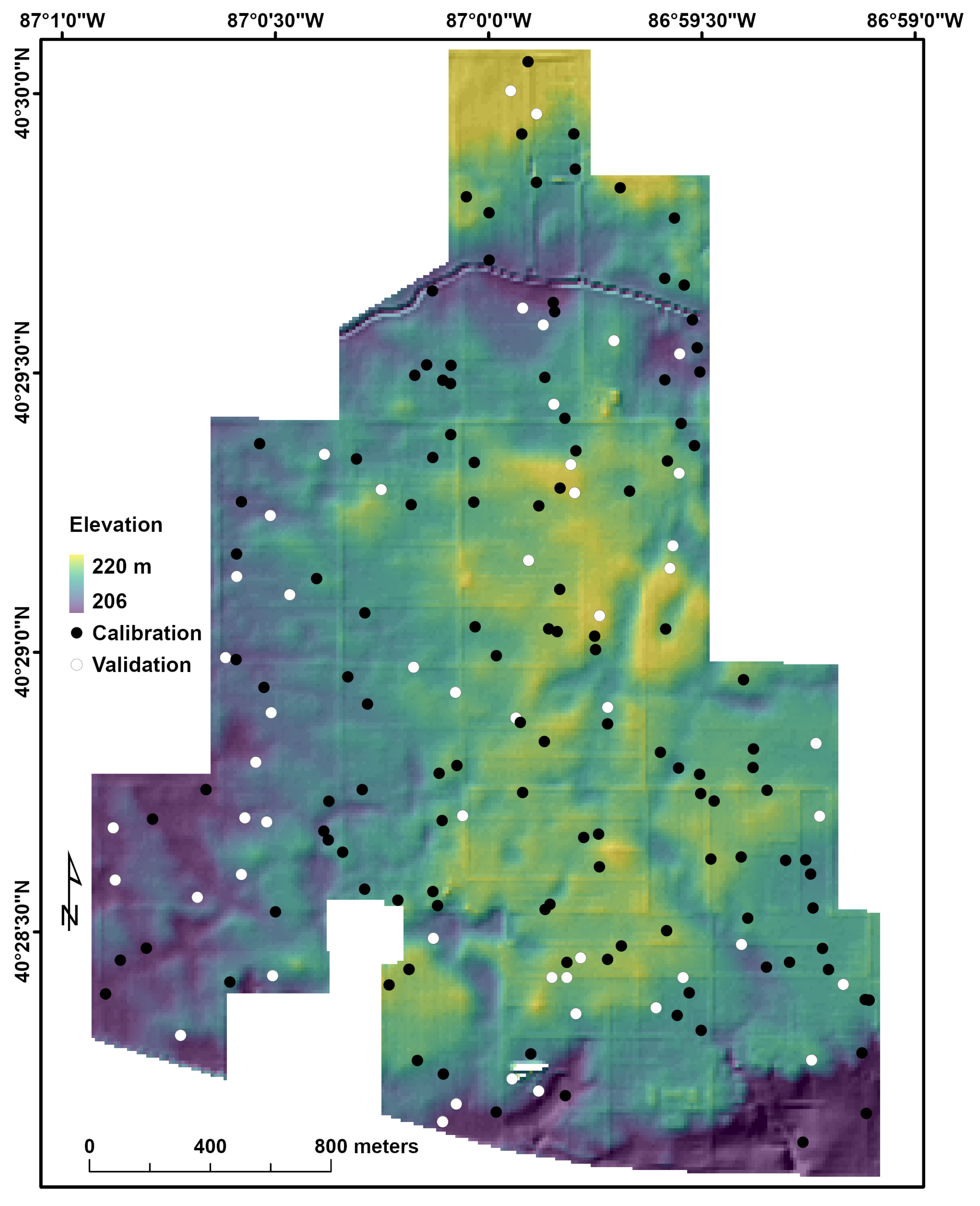
2.1. The Study Area
2.2. Soil Sampling and Analysis
2.3. Digital Elevation Model and Terrain Attributes
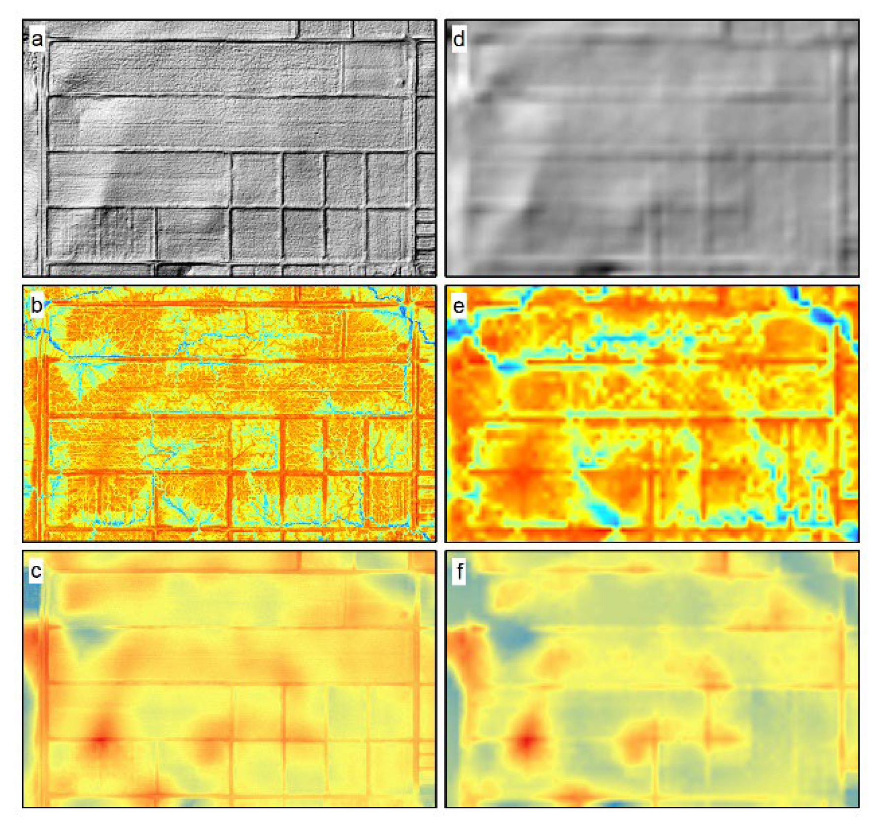
2.3.1. Digital Elevation Model
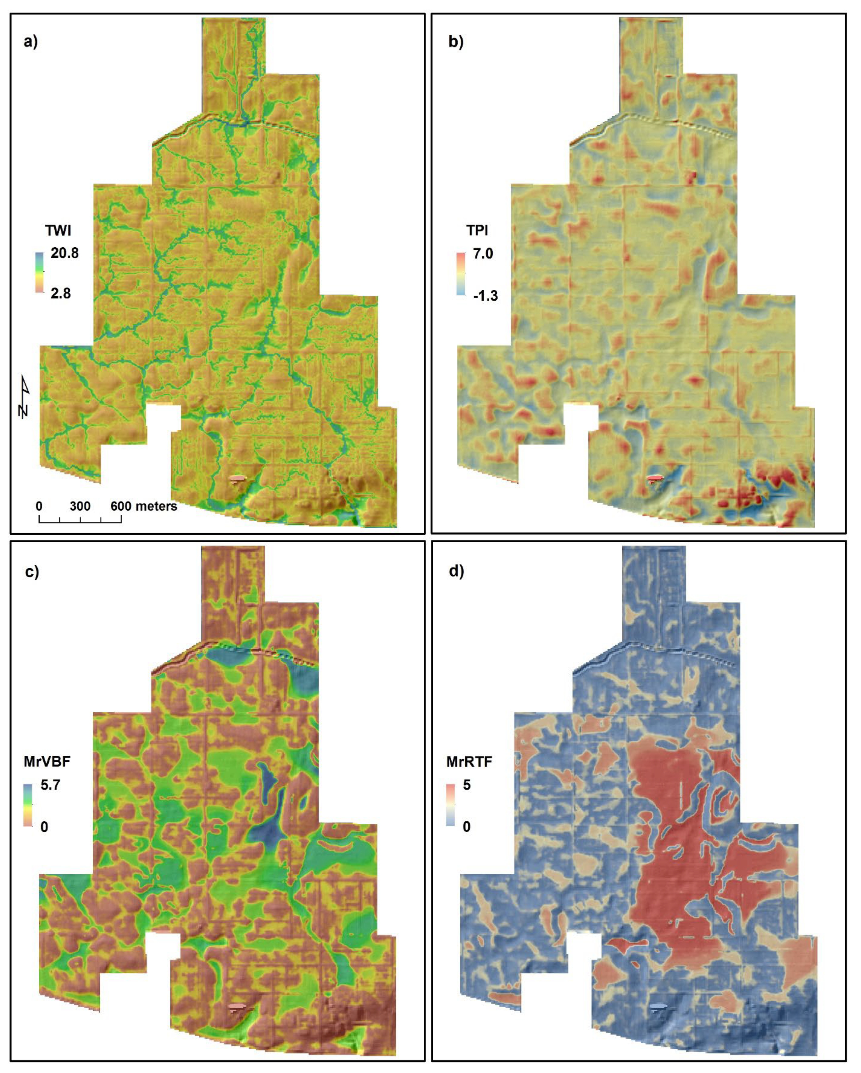
2.3.2. Terrain Attributes
Topographic Wetness Index
Topographic Position Index
Multiresolution Valley Bottom Flatness and Multiresolution Ridge Top Flatness
2.4. Data from the Soil Survey Geographic Database
2.5. Spatial Prediction Models
2.6. Validation of Model Performance
3. Results and Discussion
3.1. Descriptive Statistics
3.2. Spatial Trend Modeling
3.3. Variogram of Model Residuals
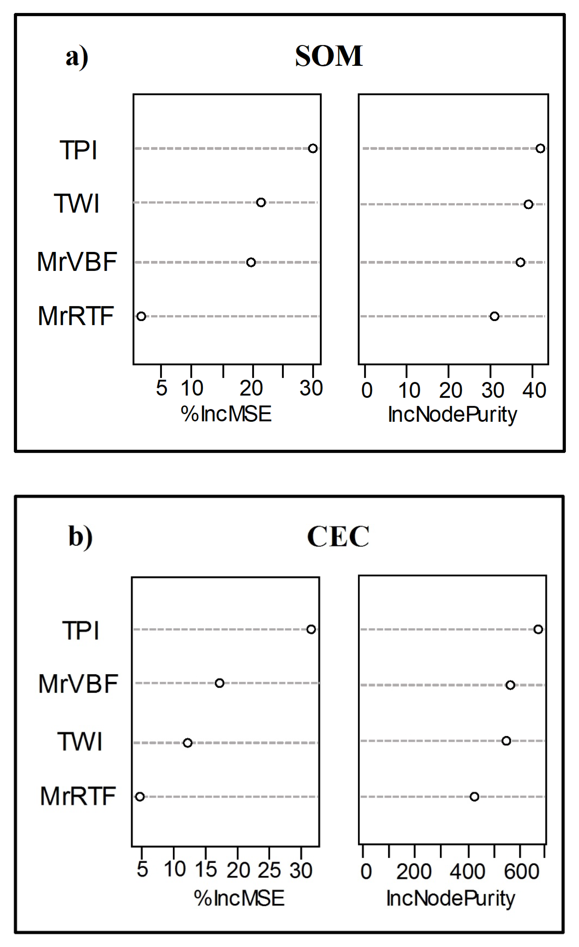
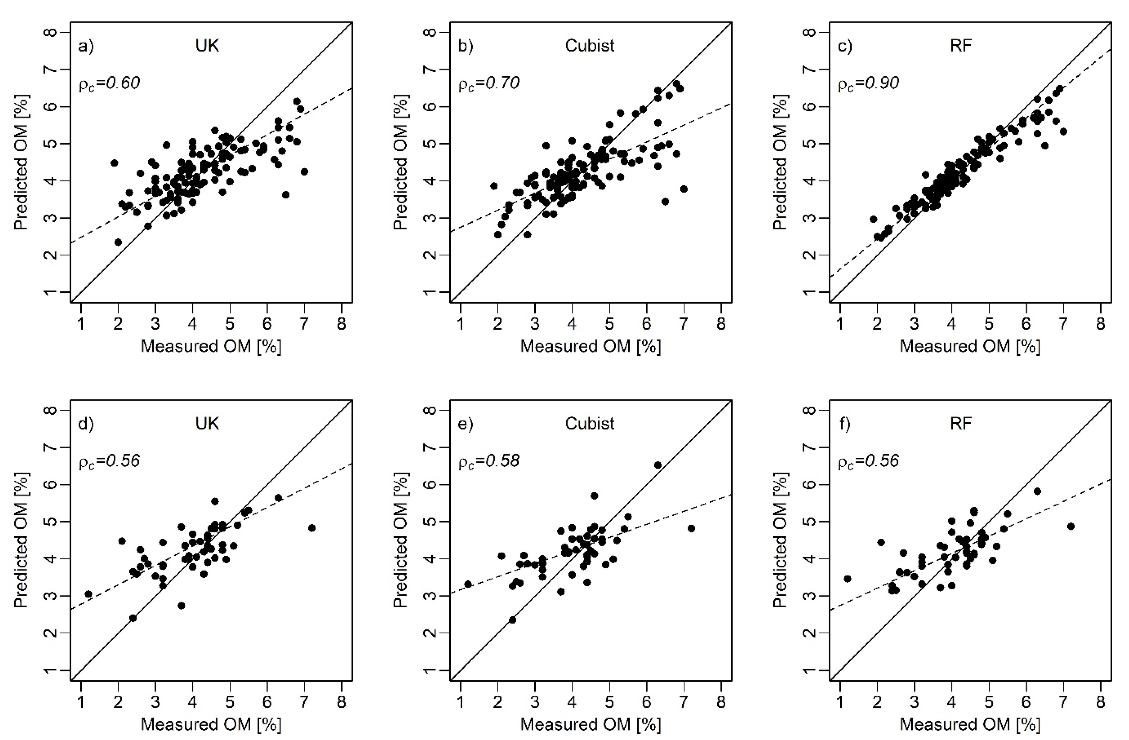
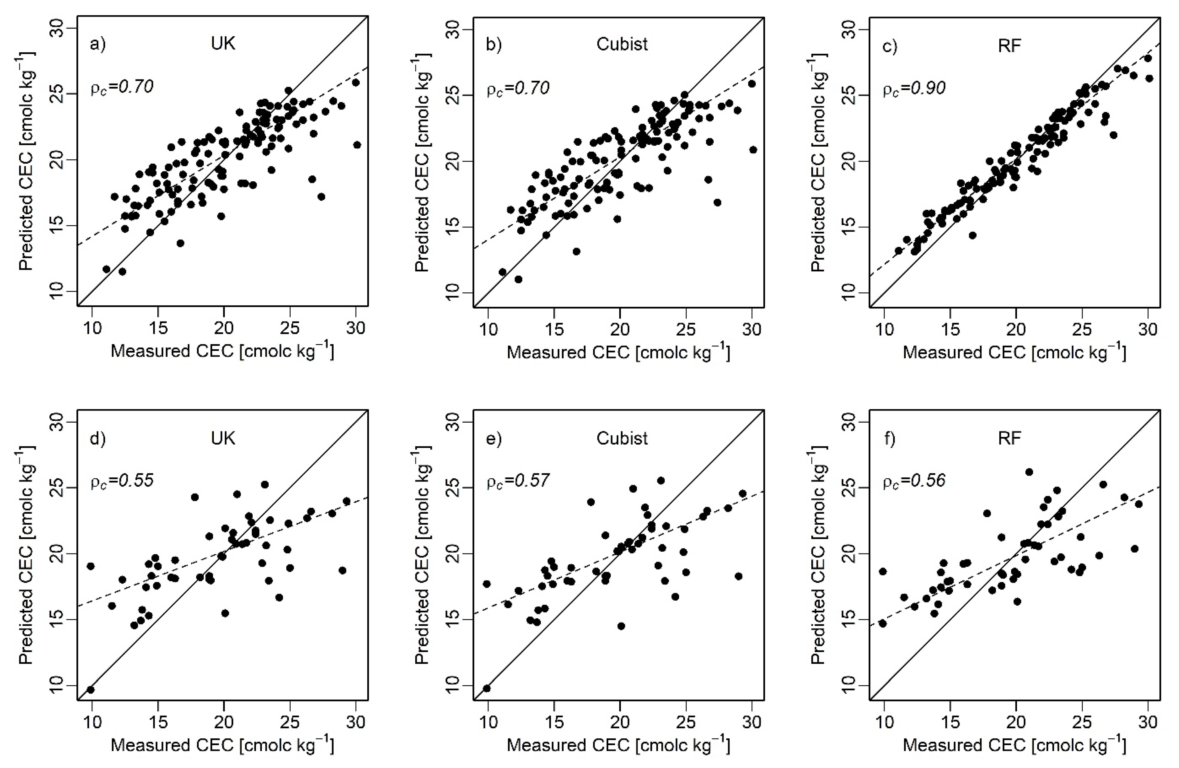
3.4. Predictive Model Performance
3.5. Organic Matter Content and Cation Exchange Capacity Distribution in the Landscape
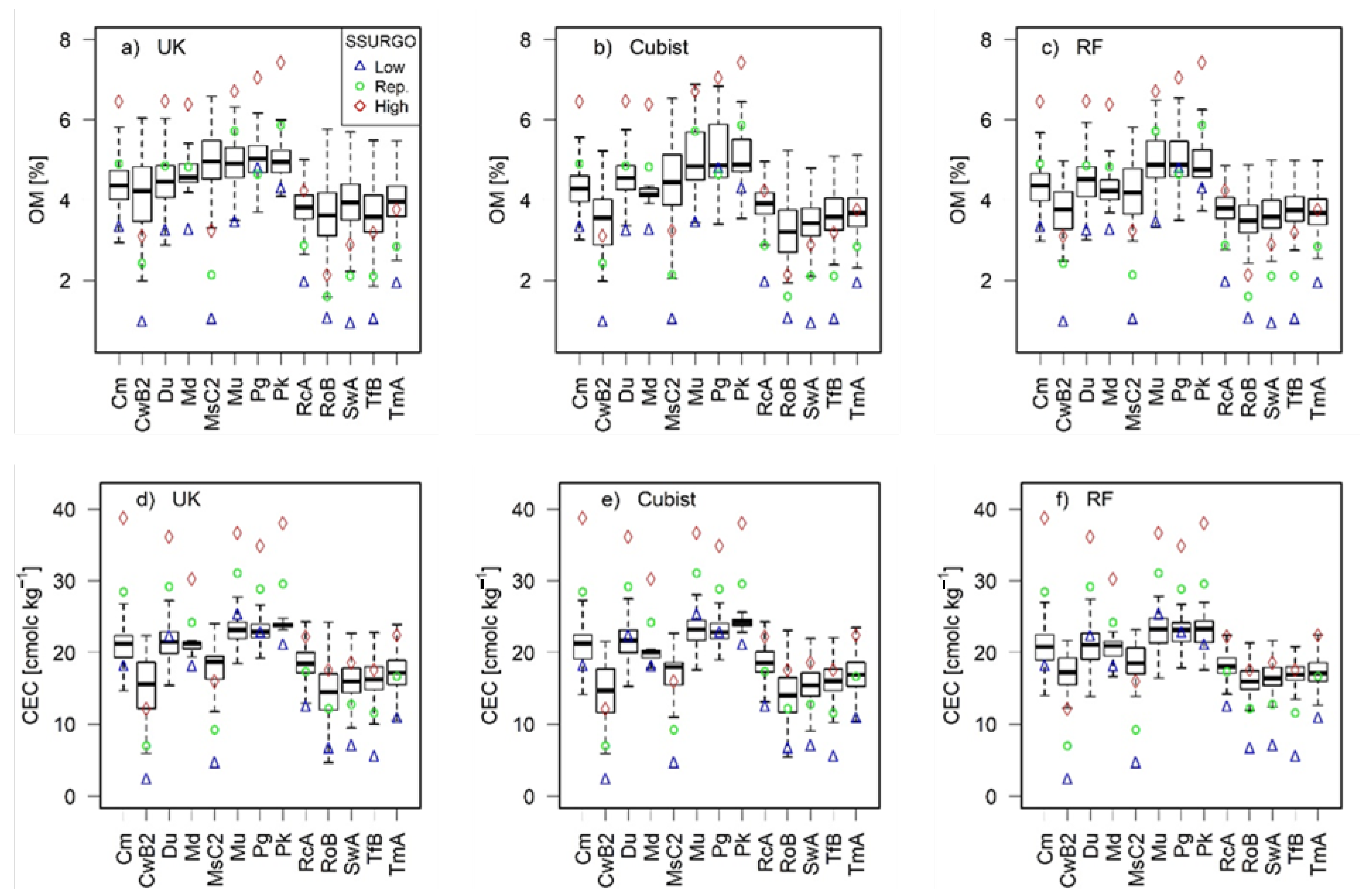
3.6. Predictive Models versus SSURGO
4. Conclusions
Author Contributions
Funding
Data Availability Statement
Acknowledgments
Conflicts of Interest
Abbreviations
References
- Jenny, H. Factors of Soil Formation: A System of Quantitative Pedology, 1st ed.; McGraw-Hill Publications in the Agricultural Sciences; McGraw-Hill: New York, NY, USA, 1941. [Google Scholar]
- Milne, G. Some suggested units of classification and mapping particularly for East African soils. Soil Res. Vitoria 1935, 4, 183–198. [Google Scholar]
- Soil Survey Staff. Natural Resources Conservation Service, United States Department of Agriculture. Soil Survey Geographic (SSURGO) Database. Available online: https://sdmdataaccess.sc.egov.usda.gov (accessed on 21 May 2021).
- Nauman, T.W.; Thompson, J.A.; Odgers, N.P.; Libohova, Z. Fuzzy disaggregation of conventional soil maps using database knowledge extraction to produce soil property maps. In Digital Soil Assessments and Beyond; Minasny, B., Malone, B.P., McBratney, A.B., Eds.; Taylor & Francis Group of CRC Press: London, UK, 2012; pp. 203–208. [Google Scholar]
- McBratney, A.B.; Santos, M.M.; Minasny, B. On digital soil mapping. Geoderma 2003, 117, 3–52. [Google Scholar] [CrossRef]
- Minasny, B.; McBratney, A.B.; Malone, B.P.; Wheeler, I. Digital mapping of soil carbon. Adv. Agron. 2013, 118, 1–47. [Google Scholar] [CrossRef]
- Arrouays, D.; Vion, I.; Kicin, J.L. Spatial analysis and modeling of topsoil carbon storage in temperate forest humic loamy soils of France. Soil Sci. 1995, 159, 191–198. [Google Scholar] [CrossRef]
- Lacoste, M.; Minasny, B.; McBratney, A.; Michot, D.; Viaud, V.; Walter, C. High resolution 3D mapping of soil organic carbon in a heterogeneous agricultural landscape. Geoderma 2014, 213, 296–311. [Google Scholar] [CrossRef]
- Grigal, D.F.; Vance, E.D. Influence of soil organic matter on forest productivity. N. Z. J. For. Sci. 2000, 30, 169–205. [Google Scholar]
- Florinsky, I.V.; Eilers, R.G.; Manning, G.R.; Fuller, L.G. Prediction of soil properties by digital terrain modelling. Environ. Model. Softw. 2002, 17, 295–311. [Google Scholar] [CrossRef]
- Grimm, R.; Behrens, T.; Märker, M.; Elsenbeer, H. Soil organic carbon concentrations and stocks on Barro Colorado Island—Digital soil mapping using Random Forests analysis. Geoderma 2008, 146, 102–113. [Google Scholar] [CrossRef]
- McKenzie, N.J.; Austin, M.P. A quantitative Australian approach to medium and small scale surveys based on soil stratigraphy and environmental correlation. Geoderma 1993, 57, 329–355. [Google Scholar] [CrossRef]
- Adhikari, K.; Hartemink, A.E. Soil organic carbon increases under intensive agriculture in the Central Sands, Wisconsin, USA. Geoderma Reg. 2017, 10, 115–125. [Google Scholar] [CrossRef]
- Chagas, C.D.S.; Carvalho Júnior, W.D.; Pinheiro, H.S.K.; Xavier, P.A.M.; Bhering, S.B.; Pereira, N.R.; Calderano Filho, B. Mapping soil cation exchange capacity in a semiarid region through predictive models and covariates from remote sensing data. Rev. Bras. Ciência Solo 2018, 42. [Google Scholar] [CrossRef]
- Mosleh, Z.; Salehi, M.H.; Jafari, A.; Borujeni, I.E.; Mehnatkesh, A. The effectiveness of digital soil mapping to predict soil properties over low-relief areas. Environ. Monit. Assess. 2016, 188, 195. [Google Scholar] [CrossRef]
- Malone, B.P.; McBratney, A.B.; Minasny, B.; Laslett, G.M. Mapping continuous depth functions of soil carbon storage and available water capacity. Geoderma 2009, 154, 138–152. [Google Scholar] [CrossRef]
- John, K.; Abraham, I.I.; Michael, K.N.; Okon, A.E.; Chapman, A.P.; Marcus, A.S. Using machine learning algorithms to estimate soil organic carbon variability with environmental variables and soil nutrient indicators in an alluvial soil. Land 2020, 9, 487. [Google Scholar] [CrossRef]
- Behrens, T.; Förster, H.; Scholten, T.; Steinrücken, U.; Spies, E.D.; Goldschmitt, M. Digital soil mapping using artificial neural networks. J. Plant Nutr. Soil. Sci. 2005, 168, 21–33. [Google Scholar] [CrossRef]
- Fathololoumi, S.; Vaezi, A.R.; Alavipanah, S.K.; Ghorbani, A.; Saurette, D.; Biswas, A. Improved digital soil mapping with multitemporal remotely sensed satellite data fusion: A case study in Iran. Sci. Total Environ. 2020, 721, 137703. [Google Scholar] [CrossRef] [PubMed]
- Mendes, W.D.S.; Demattê, J.A.M.; Salazar, D.F.U.; Amorim, M.T.A. Geostatistics or machine learning for mapping soil attributes and agricultural practices. Rev. Ceres 2020, 67, 330–336. [Google Scholar] [CrossRef]
- Zhang, G.L.; Feng, L.I.U.; Song, X.D. Recent progress and future prospect of digital soil mapping: A review. J. Integr. Agric. 2017, 16, 2871–2885. [Google Scholar] [CrossRef]
- Minasny, B.; McBratney, A.B. A conditioned Latin hypercube method for sampling in the presence of ancillary information. Comput. Geosci. 2006, 32, 1378–1388. [Google Scholar] [CrossRef]
- Peng, Y.; Xiong, X.; Adhikari, K.; Knadel, M.; Grunwald, S.; Greve, M.H. Modeling soil organic carbon at regional scale by combining multi-spectral images with laboratory spectra. PLoS ONE 2015, 10, e0142295. [Google Scholar] [CrossRef] [Green Version]
- USDA–NRCS. Soil Survey of Tippecanoe County, Indiana; United States Department of Agriculture, Natural Resources Conservation Service: Washington, DC, USA, 1998.
- Roudier, P.; Beaudette, D.E.; Hewitt, A.E. A conditioned Latin hypercube sampling algorithm incorporating operational constraints. In Digital Soil Assessments and Beyond; CRC Press: Boca Raton, FL, USA, 2012; pp. 227–231. [Google Scholar]
- R Core Team. R: A Language and Environment for Statistical Computing; R Foundation for Statistical Computing: Vienna, Austria, 2018; Available online: https://www.R-project.org/ (accessed on 30 May 2022).
- NCR. Recommended Chemical Soil Test Procedure for the North Central Region; North Central Region Publication No. 221; Missouri Agriculture Experiment Station: Columbia, MO, USA, 1998. [Google Scholar]
- Woolpert. Indiana Statewide Lidar 2017 B17 West–Airborne Lidar Report. Available online: https://lidar.jinha.org/ (accessed on 10 June 2021).
- INDOT. Indiana Geospatial Coordinate System, Version 1.05; Indiana Department of Transportation (INDOT), Aerial and Land Survey Office: Indianapolis, IN, USA, 2016.
- Winzeler, H.E.; Owens, P.R.; Joern, B.C.; Camberato, J.J.; Lee, B.D.; Anderson, D.E.; Smith, D.R. Potassium fertility and terrain attributes in a Fragiudalf drainage catena. Soil. Sci. Soc. Am. J. 2008, 72, 1311–1320. [Google Scholar] [CrossRef] [Green Version]
- Redlands, California, USA, C.E.S.R.I. ArcGIS Desktop: Release 10.6. 2011. Available online: https://esri.com (accessed on 30 May 2022).
- Soil Science Division Staff. Soil survey manual. In USDA Handbook 18; Ditzler, C., Scheffe, K., Monger, H.C., Eds.; Government Printing Office: Washington, DC, USA, 2017. [Google Scholar]
- Suleymanov, A.; Abakumov, E.; Suleymanov, R.; Gabbasova, I.; Komissarov, M. The Soil Nutrient Digital Mapping for Precision Agriculture Cases in the Trans-Ural Steppe Zone of Russia Using Topographic Attributes. ISPRS Int. J. Geo-Inf. 2021, 10, 243. [Google Scholar] [CrossRef]
- Conrad, O.; Bechtel, B.; Bock, M.; Dietrich, H.; Fischer, E.; Gerlitz, L.; Wehberg, J.; Wichmann, V.; Böhner, J. System for automated geoscientific analyses (SAGA) v. 2.1.4. Geosci. Model. Dev. Discuss. 2015, 8, 2271–2312. [Google Scholar] [CrossRef] [Green Version]
- Weiss, A. Topographic position and landforms analysis. In Proceedings of the Annual Meeting of ESRI User Conference, San Diego, CA, USA, 9–13 July 2001; Available online: http://www.jennessent.com/downloads/tpi-poster-tnc18×22.pdf (accessed on 12 December 2020).
- Gallant, J.C.; Dowling, T.I. A multiresolution index of valley bottom flatness for mapping depositional areas. Water Resour. Res. 2003, 39. [Google Scholar] [CrossRef]
- Soil Survey Staff. Natural Resources Conservation Service, United States Department of Agriculture. Web Soil Survey. Available online: https://websoilsurvey.nrcs.usda.gov/ (accessed on 12 December 2020).
- Libohova, Z.; Odgers, N.P.; Ashtekar, J.; Owens, P.R.; Thompson, J.A.; Hempel, J. Some challenges on quantifying soil property predictions uncertainty for the GlobalSoilMap using legacy data. In Digital Soil Mapping Across Paradigms, Scales and Boundaries; Zhang, G.L., Brus, D., Liu, F., Song, X.D., Lagacherie, P., Eds.; Springer: Singapore, 2016; pp. 131–140. [Google Scholar] [CrossRef]
- Franzmeier, D.P.; Steinhardt, G.C.; Crum, J.R.; Norton, L.D. Soil Characterization in Indiana: I. Field and Laboratory Procedures; West Lafayette, Indiana with cooperation of the Soil Conservation Service, U.S. Department of Agriculture. Research Bulletin No. 943; Department of Agronomy, Agriculture Experiment Stations, Purdue University: West Lafayette, IN, USA, 1977. [Google Scholar]
- Soil Survey Staff. Kellogg Soil Survey Laboratory Methods Manual; Soil Survey Investigations Report No. 42, Version 5.0.; Burt, R., Soil Survey Staff, Eds.; U.S. Department of Agriculture, Natural Resources Conservation Service: Washington, DC, USA, 2014.
- R Package, Version 1.0. Ithir: Soil Data and Some Useful Associated Functions, R Package: Sydney, Australia, 2018.
- Malone, B.P.; Minasny, B.; McBratney, A.B. Using R for Digital Soil Mapping; Springer International Publishing: Basel, Switzerland, 2017. [Google Scholar] [CrossRef]
- Adhikari, K.; Hartemink, A.E.; Minasny, B.; Bou Kheir, R.; Greve, M.B.; Greve, M.H. Digital mapping of soil organic carbon contents and stocks in Denmark. PLoS ONE 2014, 9, e105519. [Google Scholar] [CrossRef]
- Bishop, T.F.; McBratney, A.B.; Laslett, G.M. Modelling soil attribute depth functions with equal-area quadratic smoothing splines. Geoderma 1991, 91, 27–45. [Google Scholar] [CrossRef]
- Hengl, T.; Heuvelink, G.B.; Rossiter, D.G. About regression-kriging: From equations to case studies. Comput. Geosci. 2007, 33, 1301–1315. [Google Scholar] [CrossRef]
- Gräler, B.; Pebesma, E.; Heuvelink, G. Spatio-Temporal Interpolation using gstat. RFID J. 2016, 8, 204–218. [Google Scholar] [CrossRef]
- Quinlan, J.R. Learning with continuous classes. In Proceedings of the Australian Joint Conference on Artificial Intelligence, Hobart, Australia, 16–18 November 1992; pp. 343–348. [Google Scholar]
- Kuhn, M.; Quinlan, R. Cubist: Rule and Instance Based Regression Modeling. R Package Version 0.2.2. Available online: https://CRAN.R-project.org/package=Cubist (accessed on 12 December 2020).
- Breiman, L. Random forests. Mach. Learn. 2001, 45, 5–32. [Google Scholar] [CrossRef] [Green Version]
- Forkuor, G.; Hounkpatin, O.K.; Welp, G.; Thiel, M. High resolution mapping of soil properties using remote sensing variables in south-western Burkina Faso: A comparison of machine learning and multiple linear regression models. PLoS ONE 2017, 12, e0170478. [Google Scholar] [CrossRef]
- Liaw, A.; Wiener, M. Classification and regression by random Forest. R News 2002, 2, 18–22. [Google Scholar]
- Lawrence, I.; Lin, K. A concordance correlation coefficient to evaluate reproducibility. Biometrics 1989, 45, 255–268. [Google Scholar] [CrossRef]
- McBride, G.B. A Proposal for Strength-of-Agreement Criteria for Lin’s; Concordance Correlation Coefficient; National Institute of Water and Atmospheric Research Ltd.: Hamilton, New Zealand, 2005; Available online: https://www.medcalc.org/download/pdf/McBride2005.pdf (accessed on 12 December 2020).
- Wiesmeier, M.; Barthold, F.; Blank, B.; Kögel-Knabner, I. Digital mapping of soil organic matter stocks using Random Forest modeling in a semi-arid steppe ecosystem. Plant Soil 2011, 340, 7–24. [Google Scholar] [CrossRef]
- Cambardella, C.A.; Moorman, T.B.; Novak, J.M.; Parkin, T.B.; Karlen, D.L.; Turco, R.F.; Konopka, A.E. Field-scale variability of soil properties in central Iowa soils. Soil Sci. Soc. Am. J. 1994, 58, 1501–1511. [Google Scholar] [CrossRef]
- Keskin, H.; Grunwald, S. Regression kriging as a workhorse in the digital soil mapper’s toolbox. Geoderma 2018, 326, 22–41. [Google Scholar] [CrossRef]
- Rossi, J.; Govaerts, A.; De Vos, B.; Verbist, B.; Vervoort, A.; Poesen, J.; Muys, B.; Deckers, J. Spatial structures of soil organic carbon in tropical forests—A case study of Southeastern Tanzania. Catena 2009, 77, 19–27. [Google Scholar] [CrossRef]
- Greve, M.H.; Greve, M.B.; Kheir, R.B.; Bøcher, P.K.; Larsen, R.; McCloy, K. Comparing decision tree modeling and indicator Kriging for mapping the extent of organic soils in Denmark. In Digital Soil Mapping; Springer: Dordrecht, The Netherlands, 2010; pp. 267–280. [Google Scholar]
- Nabiollahi, K.; Eskandari, S.; Taghizadeh-Mehrjardi, R.; Kerry, R.; Triantafilis, J. Assessing soil organic carbon stocks under land-use change scenarios using random forest models. Carbon Manag. 2019, 10, 63–77. [Google Scholar] [CrossRef]
- Nussbaum, M.; Spiess, K.; Baltensweiler, A.; Grob, U.; Keller, A.; Greiner, L.; Schaepman, M.E.; Papritz, A. Evaluation of digital soil mapping approaches with large sets of environmental covariates. Soil 2018, 4, 1–22. [Google Scholar] [CrossRef] [Green Version]
- Rentschler, T.; Werban, U.; Ahner, M.; Behrens, T.; Gries, P.; Scholten, T.; Teuber, S.; Schmidt, K. 3D mapping of soil organic carbon content and soil moisture with multiple geophysical sensors and machine learning. Vadose Zone J. 2020, 19, e20062. [Google Scholar] [CrossRef]
- Rossel, R.V.; Walvoort, D.J.J.; McBratney, A.B.; Janik, L.J.; Skjemstad, J.O. Visible, near infrared, mid infrared or combined diffuse reflectance spectroscopy for simultaneous assessment of various soil properties. Geoderma 2006, 131, 59–75. [Google Scholar] [CrossRef]
- Guillaume, T.; Bragazza, L.; Levasseur, C.; Libohova, Z.; Sinaj, S. Long-term soil organic carbon dynamics in temperate cropland-grassland systems. Agric. Ecosyst. Environ. 2021, 305, 107184. [Google Scholar] [CrossRef]
- Caley, G.K.; Hengl, T.; Gräler, B.; Meyer, H.; Magney, T.S.; Brown, D.J. Spatio-temporal interpolation of soil water, temperature, and electrical conductivity in 3D+ T: The Cook Agronomy Farm data set. Spat. Stat. 2015, 14, 70–90. [Google Scholar] [CrossRef]
- Schöning, I.; Totsche, K.U.; Kögel-Knabner, I. Small scale spatial variability of organic carbon stocks in litter and solum of a forested Luvisol. Geoderma 2006, 136, 631–642. [Google Scholar] [CrossRef]
- Trangmar, B.B.; Yost, R.S.; Uehara, G. Application of geostatistics to spatial studies of soil properties. Adv. Agron. 1985, 38, 45–94. [Google Scholar] [CrossRef]
- Mason, E.; Sulaeman, Y. Comparison of three models for predicting the spatial distribution of soil organic carbon in Boalemo Regency, Sulawesi. J. Ilmu. Tanah. Dan. Lingkung. 2016, 18, 42–48. [Google Scholar] [CrossRef]
- Pouladi, N.; Møller, A.B.; Tabatabai, S.; Greve, M.H. Mapping soil organic matter contents at field level with Cubist, Random Forest and kriging. Geoderma 2019, 342, 85–92. [Google Scholar] [CrossRef]
- Nauman, T.W.; Thompson, J.A. Semi-automated disaggregation of conventional soil maps using knowledge driven data mining and classification trees. Geoderma 2014, 213, 385–399. [Google Scholar] [CrossRef]
- Geza, M.; McCray, J.E. Effects of soil data resolution on SWAT model stream flow and water quality predictions. J. Environ. Manag. 2008, 88, 393–406. [Google Scholar] [CrossRef]
- De Vos, B.; Lettens, S.; Muys, B.; Deckers, J.A. Walkley–Black analysis of forest soil organic carbon: Recovery, limitations and uncertainty. Soil Use Manag. 2007, 23, 221–229. [Google Scholar] [CrossRef]
- Shamrikova, E.V.; Kondratenok, B.M.; Tumanova, E.A.; Vanchikova, E.V.; Lapteva, E.M.; Zonova, T.V.; Lu-Lyan-Min, E.I.; Davydova, A.P.; Libohova, Z.; Suvannang, N. Transferability between soil organic matter measurement methods for database harmonization. Geoderma 2022, 412, 115547. [Google Scholar] [CrossRef]
- Bot, A.; Benites, J. The Importance of Soil Organic Matter: Key to Drought-Resistant Soil and Sustained Food Production; Food and Agriculture Organization of the United Nations: Rome, Italy, 2005; Volume 80. [Google Scholar]
- Toni, L.R.M.; de Santana, H.; Zaia, C.T.B.V.; Zaia, D.A.M. Seasonal and depth effects on some parameters of a forest soil. Semin. Exact Technol. Sci. 2009, 30, 19–32. [Google Scholar] [CrossRef] [Green Version]
- Libohova, Z.; Seybold, C.; Adhikari, K.; Wills, S.; Beaudette, D.; Peaslee, S.; Lindbo, D.; Owens, P.R. The anatomy of uncertainty for soil pH measurements and predictions: Implications for modelers and practitioners. Eur. J. Soil Sci. 2019, 70, 185–199. [Google Scholar] [CrossRef] [Green Version]


| SSURGO Soil Map Unit | SOM | CEC | ||||||
|---|---|---|---|---|---|---|---|---|
| Area | Low | Rep. | High | Low | Mean | High | ||
| % | % | cmolc kg−1 | ||||||
| Cm | Chalmers silty clay loam | 33.9 | 3.5 | 4.9 | 6.5 | 18.2 | 28.5 | 38.8 |
| CwB2 | Crosby-Miami silt loams | 0.4 | 1.0 | 2.4 | 3.1 | 2.5 | 7.0 | 12.2 |
| Du | Drummer soils | 17.6 | 3.3 | 4.9 | 6.5 | 22.4 | 29.2 | 36.2 |
| Md | Mahalasville-Treaty complex | 0.2 | 3.3 | 4.8 | 6.4 | 18.2 | 24.2 | 30.3 |
| MsC2 | Miami silt loam | 0.2 | 1.1 | 2.1 | 3.3 | 4.7 | 9.2 | 16.0 |
| Mu | Milford silty clay loam | 4.2 | 3.5 | 5.7 | 6.7 | 25.4 | 31.1 | 36.7 |
| Pg | Pella silty clay loam | 1.6 | 4.8 | 4.7 | 7.1 | 22.9 | 28.9 | 34.9 |
| Pk | Peotone silty clay loam | 0.6 | 4.3 | 5.9 | 7.4 | 21.2 | 29.6 | 38.1 |
| RcA | Raub-Brenton complex | 22.1 | 1.9 | 2.9 | 4.2 | 12.5 | 17.4 | 22.3 |
| RoB | Rockfield silt loam | 4.6 | 1.1 | 1.6 | 2.1 | 6.7 | 12.2 | 17.6 |
| SwA | Starks-Fincastle complex | 3.6 | 0.9 | 2.1 | 2.9 | 7.1 | 12.8 | 18.6 |
| TfB | Throckmorton silt loam | 1.4 | 1.1 | 2.1 | 3.2 | 5.6 | 11.6 | 17.6 |
| TmA | Toronto-Millbrook complex | 8.7 | 1.9 | 2.9 | 3.8 | 10.9 | 16.7 | 22.5 |
| Ua * | Udorthents, loamy | 0.9 | - | - | - | - | - | - |
| Statistical Index | SOM | CEC | ||||
|---|---|---|---|---|---|---|
| Whole Dataset | Calibration | Validation | Whole Dataset | Calibration | Validation | |
| % | cmolc kg−1 | |||||
| Minimum | 1.2 | 1.9 | 1.2 | 9.9 | 11.1 | 9.9 |
| 1st Quartile | 3.5 | 3.5 | 3.2 | 16.2 | 16.5 | 14.9 |
| Median | 4.0 | 4.0 | 4.2 | 20.1 | 20.1 | 20.1 |
| Mean | 4.2 | 4.2 | 4.0 | 19.9 | 20.1 | 19.5 |
| 3rd Quartile | 4.8 | 4.9 | 4.6 | 23.2 | 23.3 | 23.0 |
| Maximum | 7.2 | 7.0 | 7.2 | 30.1 | 30.1 | 29.3 |
| Standard Deviation | 1.1 | 1.2 | 1.1 | 4.6 | 4.5 | 4.9 |
| Terrain Attributes | Dataset | Statistical Index | ||||||
|---|---|---|---|---|---|---|---|---|
| Minimum | 1st Quartile | Median | Mean | 3rd Quartile | Maximum | Standard Deviation | ||
| TWI | Whole dataset | 5.29 | 7.37 | 8.69 | 9.39 | 10.71 | 18.73 | 2.64 |
| Calibration | 5.29 | 7.37 | 8.72 | 9.58 | 10.81 | 18.73 | 2.84 | |
| Validation | 6.04 | 7.51 | 8.41 | 8.93 | 10.25 | 15.31 | 2.04 | |
| TPI | Whole dataset | −0.46 | −0.11 | −0.03 | −0.01 | 0.09 | 0.71 | 0.18 |
| Calibration | −0.45 | −0.11 | −0.04 | 0.00 | 0.09 | 0.62 | 0.18 | |
| Validation | −0.46 | −0.10 | −0.03 | −0.01 | 0.07 | 0.71 | 0.19 | |
| MrVBF | Whole dataset | 0.00 | 0.37 | 1.60 | 1.62 | 2.75 | 5.24 | 1.33 |
| Calibration | 0.00 | 0.46 | 1.74 | 1.72 | 2.80 | 4.96 | 1.28 | |
| Validation | 0.01 | 0.17 | 0.65 | 1.39 | 2.63 | 5.24 | 1.44 | |
| MrRTF | Whole dataset | 0.00 | 0.14 | 0.74 | 1.64 | 2.98 | 4.99 | 1.76 |
| Calibration | 0.00 | 0.15 | 1.16 | 1.84 | 3.65 | 4.99 | 1.84 | |
| Validation | 0.00 | 0.12 | 0.47 | 1.18 | 1.50 | 4.99 | 1.47 | |
| Soil Property | DSM Model | Semi-Variogram Model | Nugget | Sill | Nugget:Sill | Range (m) |
|---|---|---|---|---|---|---|
| SOM | UK | Spherical | 0.22 | 0.43 | 0.51 | 126.12 |
| Cubist | Exponential | 0.18 | 0.39 | 0.46 | 175.00 | |
| RF | Exponential | 0.08 | 0.11 | 0.72 | 176.29 | |
| CEC | UK | Spherical | 5.46 | 5.70 | 0.96 | 229.00 |
| Cubist | Spherical | 5.23 | 5.86 | 0.89 | 307.60 | |
| RF | Spherical | 1.16 | 1.41 | 0.82 | 405.50 |
| Prediction Model | SOM | CEC | |||||||
|---|---|---|---|---|---|---|---|---|---|
| R2 | Bias | RMSE | R2 | Bias | RMSE | ||||
| % | cmolc kg−1 | ||||||||
| UK | Calibration | 0.50 | 0.00 | 0.80 | 0.60 | 0.60 | 0.00 | 2.80 | 0.70 |
| Validation | 0.44 | 0.22 | 0.83 | 0.56 | 0.39 | 0.05 | 3.74 | 0.55 | |
| Cubist | Calibration | 0.50 | 0.00 | 0.80 | 0.70 | 0.60 | 0.00 | 2.80 | 0.70 |
| Validation | 0.45 | 0.17 | 0.80 | 0.58 | 0.41 | 0.00 | 3.68 | 0.57 | |
| RF | Calibration | 0.90 | 0.00 | 0.40 | 0.90 | 0.90 | 0.00 | 1.40 | 0.90 |
| Validation | 0.45 | 0.17 | 0.80 | 0.56 | 0.44 | 0.17 | 3.62 | 0.56 | |
| SSURGO | Calibration | 0.31 | −0.14 | 1.11 | 0.56 | 0.51 | 3.88 | 6.06 | 0.53 |
| Validation | 0.40 | −0.03 | 0.99 | 0.62 | 0.56 | 3.85 | 5.78 | 0.58 | |
| Statistical Index | SOM | CEC | ||||||
|---|---|---|---|---|---|---|---|---|
| UK | Cubist | RF | SSURGO | UK | Cubist | RF | SSURGO | |
| % | cmolc kg−1 | |||||||
| Minimum | 0.9 | 1.9 | 2.4 | 1.6 | 1.1 | 5.2 | 11.9 | 7.0 |
| 1st Quartile | 3.8 | 3.8 | 3.7 | 2.9 | 17.7 | 17.6 | 17.5 | 17.4 |
| Median | 4.2 | 4.2 | 4.1 | 4.9 | 20.0 | 19.9 | 19.4 | 28.5 |
| Mean | 4.2 | 4.2 | 4.2 | 4.0 | 19.6 | 19.6 | 19.7 | 23.5 |
| 3rd Quartile | 4.7 | 4.6 | 4.6 | 4.9 | 22.0 | 22.1 | 21.8 | 28.5 |
| Maximum | 7.8 | 7.2 | 6.5 | 5.9 | 28.6 | 28.1 | 27.8 | 31.1 |
| Standard Deviation | 0.7 | 0.8 | 0.7 | 1.2 | 3.2 | 3.3 | 2.8 | 6.6 |
Publisher’s Note: MDPI stays neutral with regard to jurisdictional claims in published maps and institutional affiliations. |
© 2022 by the authors. Licensee MDPI, Basel, Switzerland. This article is an open access article distributed under the terms and conditions of the Creative Commons Attribution (CC BY) license (https://creativecommons.org/licenses/by/4.0/).
Share and Cite
Rahmani, S.R.; Ackerson, J.P.; Schulze, D.; Adhikari, K.; Libohova, Z. Digital Mapping of Soil Organic Matter and Cation Exchange Capacity in a Low Relief Landscape Using LiDAR Data. Agronomy 2022, 12, 1338. https://doi.org/10.3390/agronomy12061338
Rahmani SR, Ackerson JP, Schulze D, Adhikari K, Libohova Z. Digital Mapping of Soil Organic Matter and Cation Exchange Capacity in a Low Relief Landscape Using LiDAR Data. Agronomy. 2022; 12(6):1338. https://doi.org/10.3390/agronomy12061338
Chicago/Turabian StyleRahmani, Shams R., Jason P. Ackerson, Darrell Schulze, Kabindra Adhikari, and Zamir Libohova. 2022. "Digital Mapping of Soil Organic Matter and Cation Exchange Capacity in a Low Relief Landscape Using LiDAR Data" Agronomy 12, no. 6: 1338. https://doi.org/10.3390/agronomy12061338
APA StyleRahmani, S. R., Ackerson, J. P., Schulze, D., Adhikari, K., & Libohova, Z. (2022). Digital Mapping of Soil Organic Matter and Cation Exchange Capacity in a Low Relief Landscape Using LiDAR Data. Agronomy, 12(6), 1338. https://doi.org/10.3390/agronomy12061338