
A Flood Mapping Method for Land Use Management in Small-Size Water Bodies: Validation of Spectral Indexes and a Machine Learning Technique


Abstract
:1. Introduction
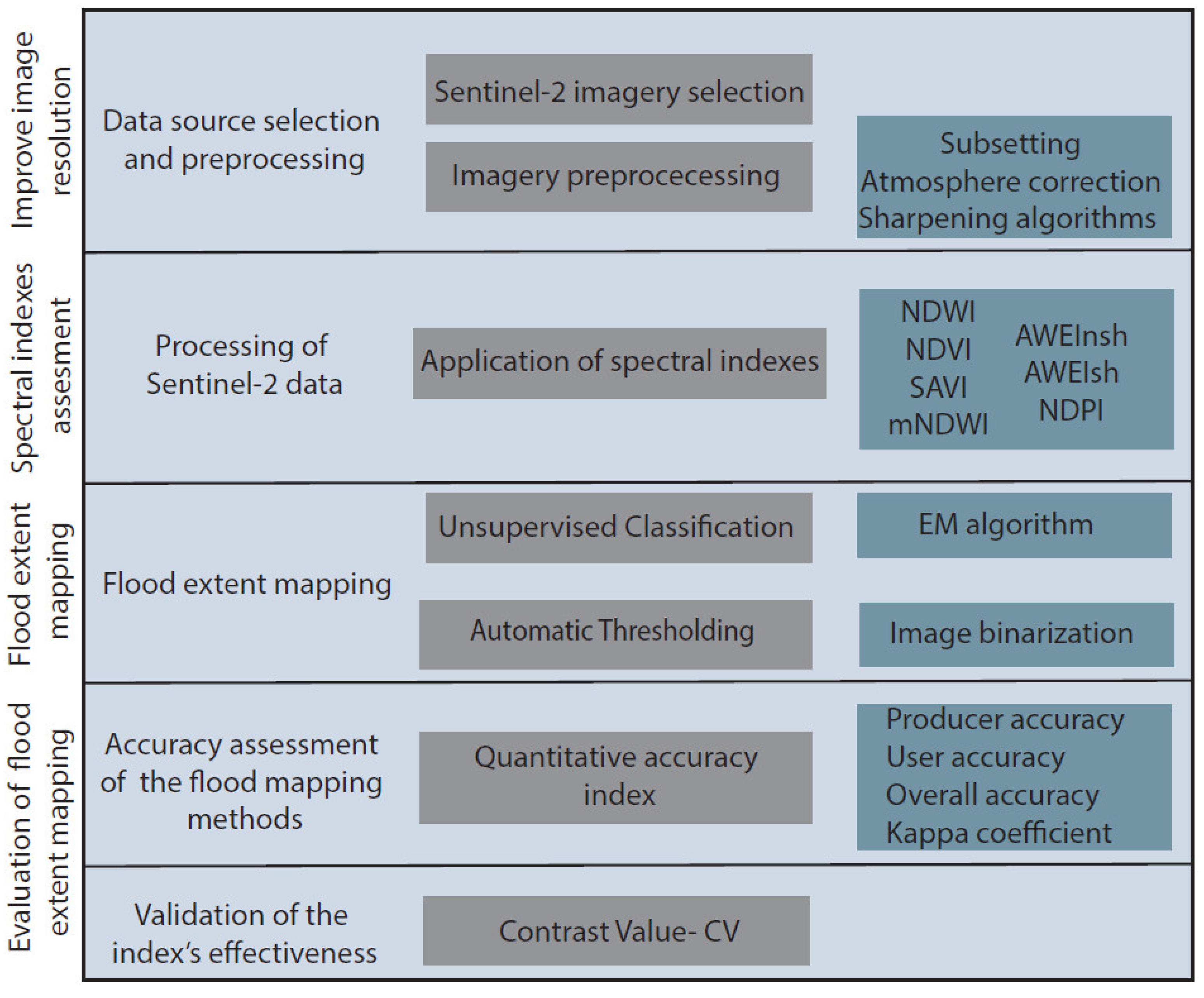
2. Methods
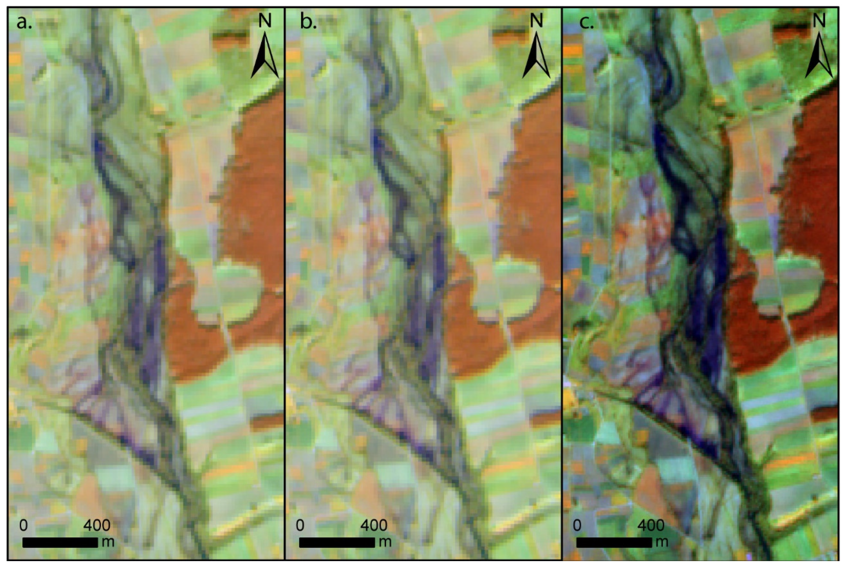
2.1. Data Source Selection and Pre-Processing
2.2. Processing of Sentinel-2 Data: Spectral Indices
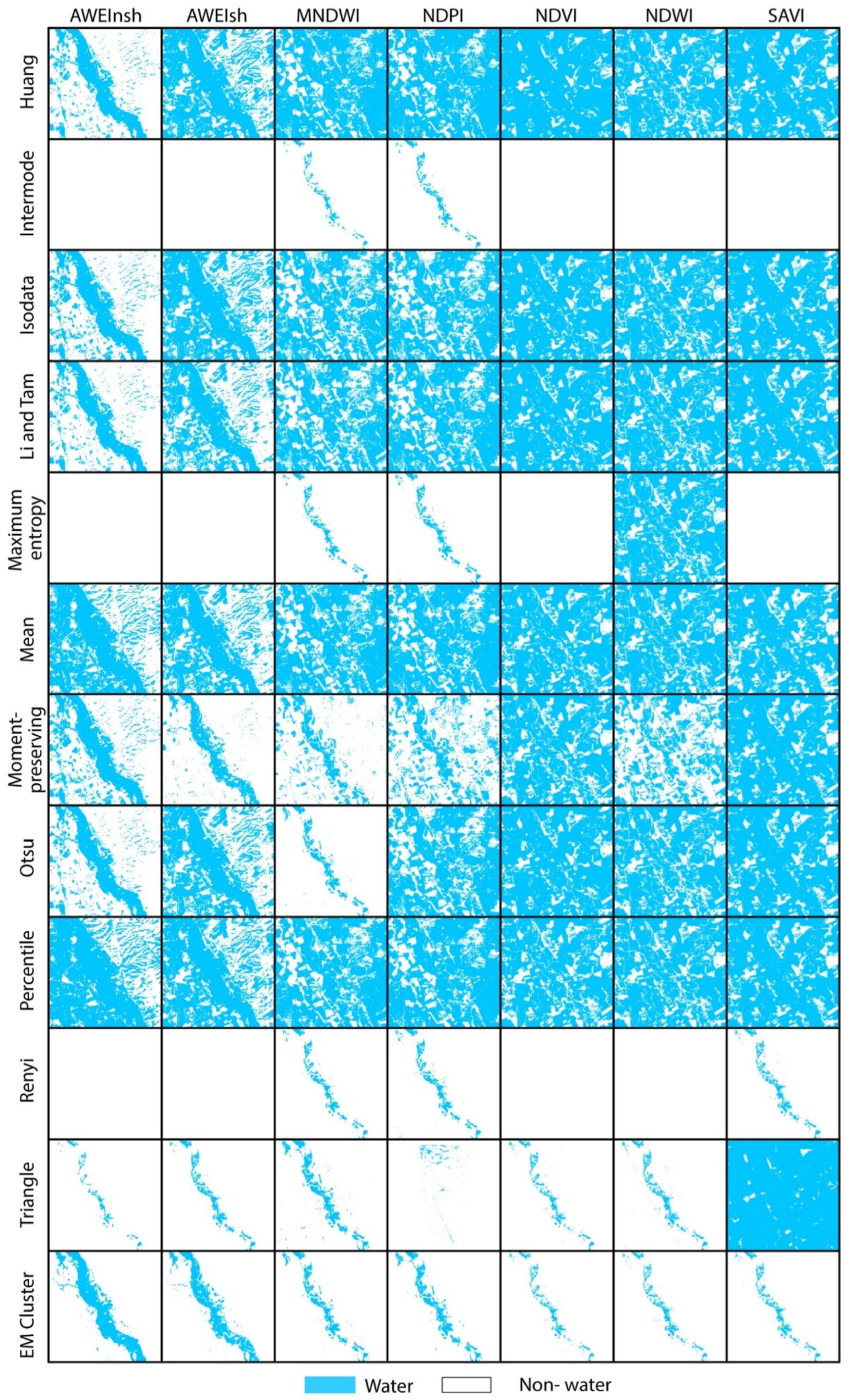
2.3. Flood Extent Mapping
2.4. Accuracy Assessment of the Flood Mapping Methods
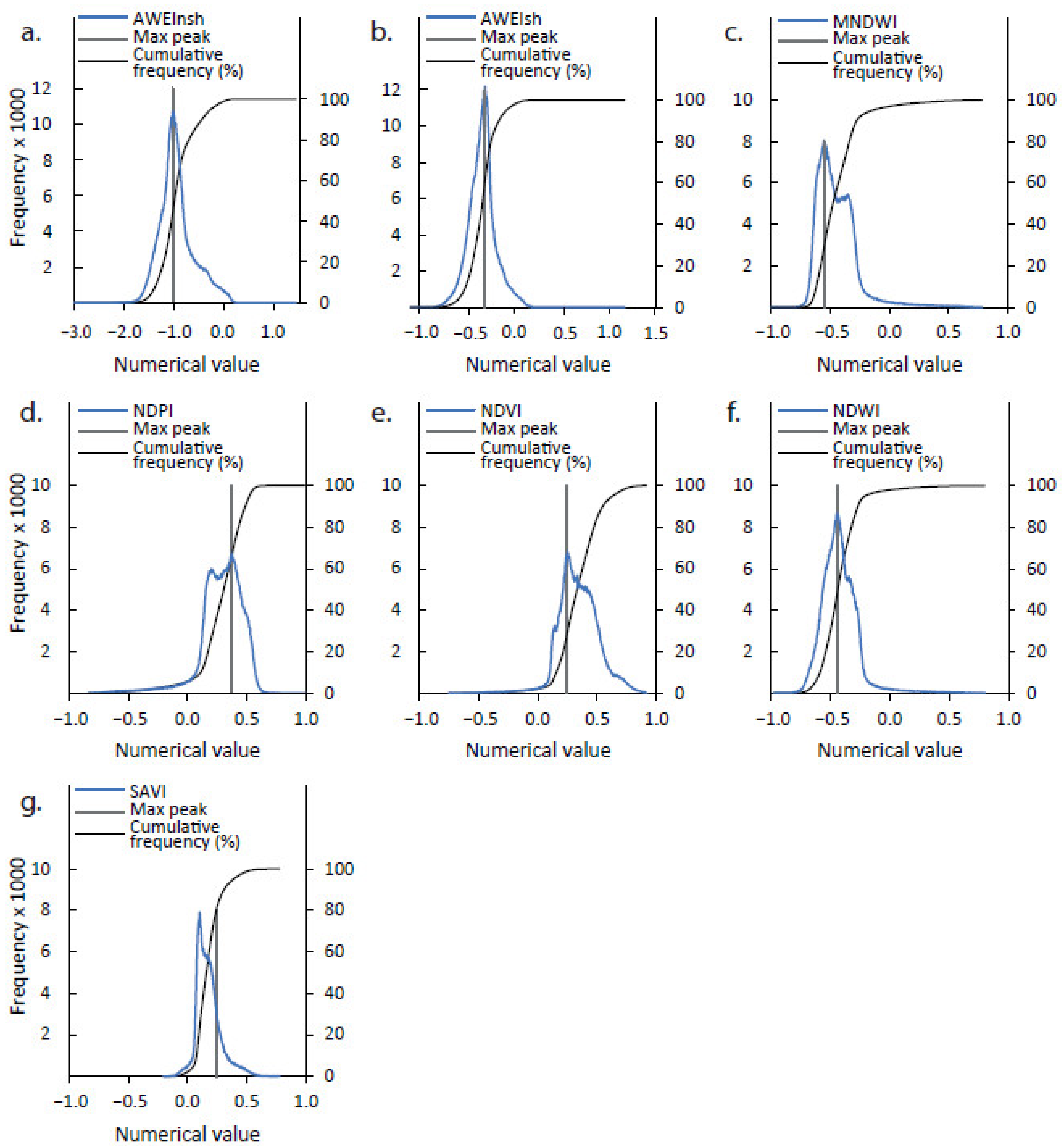
2.5. Validation of the Index’s Effectiveness
3. Results
3.1. Image Processing
3.2. Application of the Spectral Indices and Effectiveness Validation
3.3. Flood Extent Mapping Performance
4. Discussion
5. Conclusions
Author Contributions
Funding
Acknowledgments
Conflicts of Interest
Appendix A
References
- European Court of Auditors—ECA. Floods Directive: Progress in Assessing Risks, While Planning and Implementation Need to Improve; Special Report No 25, 2018; ECA: Luxembourg, 2019. [Google Scholar] [CrossRef]
- Alfieri, L.; Burek, P.; Feyen, L.; Forzieri, G. Global warming increases the frequency of river floods in Europe. Hydrol. Earth Syst. Sci. 2015, 19, 2247–2260. [Google Scholar] [CrossRef] [Green Version]
- Sofia, G.; Nikolopoulos, E.I. Floods and rivers: A circular causality perspective. Sci. Rep. 2020, 10, 5175. [Google Scholar] [CrossRef] [Green Version]
- Dong, Z.; Wang, G.; Amankwah, S.O.Y.; Wei, X.; Hu, Y.; Feng, A. Monitoring the summer flooding in the Poyang Lake area of China in 2020 based on Sentinel-1 data and multiple convolutional neural networks. Int. J. Appl. Earth Obs. Geoinf. 2021, 102, 102400. [Google Scholar] [CrossRef]
- Caballero, I.; Ruiz, J.; Navarro, G. Sentinel-2 satellites provide near-real time evaluation of catastrophic floods in the West Mediterranean. Water 2019, 11, 2499. [Google Scholar] [CrossRef] [Green Version]
- Goffi, A.; Stroppiana, D.; Brivio, P.A.; Bordogna, G.; Boschetti, M. Towards an automated approach to map flooded areas from Sentinel-2 MSI data and soft integration of water spectral features. Int. J. Appl. Earth Obs. Geoinf. 2020, 84, 101951. [Google Scholar] [CrossRef]
- Bijeesh, T.V.; Narasimhamurthy, K.N. Surface water detection and delineation using remote sensing images: A review of methods and algorithms. Sustain. Water Resour. Manag. 2020, 6, 68. [Google Scholar] [CrossRef]
- Sekertekin, A. Potential of global thresholding methods for the identification of surface water resources using Sentinel-2 satellite imagery and normalized difference water index. J. Appl. Remote Sens. 2019, 13, 044507. [Google Scholar] [CrossRef]
- European Space Agency. SENTINEL-2 User Handbook; European Space Agency: Paris, France, 2015; Available online: https://sentinel.esa.int/documents/247904/685211/Sentinel-2_User_Handbook (accessed on 30 July 2021).
- Jiang, W.; Ni, Y.; Pang, Z.; Li, X.; Ju, H.; He, G.; Lv, J.; Yang, K.; Fu, J.; Qin, X. An Effective Water Body Extraction Method with New Water Index for Sentinel-2 Imagery. Water 2021, 13, 1647. [Google Scholar] [CrossRef]
- Du, Y.; Zhang, Y.; Ling, F.; Wang, Q.; Li, W.; Li, X. Water Bodies’ Mapping from Sentinel-2 Imagery with Modified Normalized Difference Water Index at 10-m Spatial Resolution Produced by Sharpening the SWIR Band. Remote Sens. 2016, 8, 354. [Google Scholar] [CrossRef] [Green Version]
- Landuyt, L.; Verhoest, N.E.C.; Van Coillie, F.M.B. Flood Mapping in Vegetated Areas Using an Unsupervised Clustering Approach on Sentinel-1 and -2 Imagery. Remote Sens. 2020, 12, 3611. [Google Scholar] [CrossRef]
- Hu, P.; Zhang, Q.; Shi, P.; Chen, B.; Fang, J. Flood-induced mortality across the globe: Spatiotemporal pattern and influencing factors. Sci. Total Environ. 2018, 643, 171–182. [Google Scholar] [CrossRef]
- Zhou, Y.; Dong, J.; Xiao, X.; Xiao, T.; Yang, Z.; Zhao, G.; Zou, Z.; Qin, Y. Open Surface Water Mapping Algorithms: A Comparison of Water-Related Spectral Indices and Sensors. Water 2017, 9, 256. [Google Scholar] [CrossRef]
- Yue, H.; Li, Y.; Qian, J.; Liu, Y. A new accuracy evaluation method for water body extraction. Int. J. Remote Sens. 2020, 41, 7311–7342. [Google Scholar] [CrossRef]
- Wang, H.; Chu, Y.; Huang, Z.; Hwang, C.; Chao, N. Robust, Long-term Lake Level Change from Multiple Satellite Altimeters in Tibet: Observing the Rapid Rise of Ngangzi Co over a New Wetland. Remote Sens. 2019, 11, 558. [Google Scholar] [CrossRef] [Green Version]
- McFeeters, S.K. The use of the Normalized Difference Water Index (NDWI) in the delineation of open water features. Int. J. Remote Sens. 1996, 17, 1425–1432. [Google Scholar] [CrossRef]
- Xu, H. Modification of normalised difference water index (NDWI) to enhance open water features in remotely sensed imagery. Int. J. Remote Sens. 2006, 27, 3025–3033. [Google Scholar] [CrossRef]
- Feyisa, G.L.; Meilby, H.; Fensholt, R.; Proud, S.R. Automated Water Extraction Index: A new technique for surface water mapping using Landsat imagery. Remote Sens. Environ. 2014, 140, 23–35. [Google Scholar] [CrossRef]
- Rokni, K.; Ahmad, A.; Selamat, A.; Hazini, S. Water Feature Extraction and Change Detection Using Multitemporal Landsat Imagery. Remote Sens. 2014, 6, 4173–4189. [Google Scholar] [CrossRef] [Green Version]
- Otsu, N. Threshold selection method from gray-level histograms. IEEE Trans. Syst. Man Cybern. SMC 1979, 9, 62–66. [Google Scholar] [CrossRef] [Green Version]
- Huang, X.; Xie, C.; Fang, X.; Zhang, L. Combining Pixel-and Object-Based Machine Learning for Identification of Water-Body Types from Urban High-Resolution Remote-Sensing Imagery. IEEE J. Sel. Top. Appl. Earth Obs. Remote Sens. 2015, 8, 2097–2110. [Google Scholar] [CrossRef]
- Zhang, Q.; Zhang, P.; Hu, X. Unsupervised GRNN flood mapping approach combined with uncertainty analysis using bi-temporal Sentinel-2 MSI imageries. Int. J. Digit. Earth 2021, 14, 1561–1581. [Google Scholar] [CrossRef]
- Bhangale, U.; More, S.; Shaikh, T.; Patil, S.; More, N. Analysis of Surface Water Resources Using Sentinel-2 Imagery. Procedia Comput. Sci. 2020, 171, 2645–2654. [Google Scholar] [CrossRef]
- Acharya, T.D.; Subedi, A.; Lee, D.H. Evaluation of Water Indices for Surface Water Extraction in a Landsat 8 Scene of Nepal. Sensors 2018, 18, 2580. [Google Scholar] [CrossRef] [PubMed] [Green Version]
- Yang, X.; Zhao, S.; Qin, X.; Zhao, N.; Liang, L.; Kuenzer, C.; Mishra, D.R.; Huang, W.; Thenkabail, P.S. Mapping of Urban Surface Water Bodies from Sentinel-2 MSI Imagery at 10 m Resolution via NDWI-Based Image Sharpening. Remote Sens. 2017, 9, 596. [Google Scholar] [CrossRef] [Green Version]
- Lanaras, C.; Bioucas-Dias, J.; Galliani, S.; Baltsavias, E.; Schindler, K. Super-resolution of Sentinel-2 images: Learning a globally applicable deep neural network. ISPRS J. Photogramm. Remote Sens. 2018, 146, 305–319. [Google Scholar] [CrossRef] [Green Version]
- Gašparović, M.; Jogun, T. The effect of fusing Sentinel-2 bands on land-cover classification. Int. J. Remote Sens. 2017, 39, 822–841. [Google Scholar] [CrossRef]
- Brodu, N. Super-Resolving Multiresolution Images with Band-Independent Geometry of Multispectral Pixels. IEEE Trans. Geosci. Remote Sens. 2017, 55, 4610–4617. [Google Scholar] [CrossRef] [Green Version]
- Confederación Hidrográfica del Duero—CHD. Demarcación Hidrográfica del Duero—Revisión y Actualización de la Evaluación Preliminar del Riesgo de Inundación 2o Ciclo. Available online: https://www.chduero.es/documents/20126/704746/0_REVISION_EPRI_DUERO_MEMORIA.pdf/d42faee0-dd95-f352-f820-b150904a7131?t=1566469961152 (accessed on 20 August 2021).
- Lombana, L.; Martínez-Graña, A. Hydrogeomorphological analysis for hydraulic public domain definition: Case study in Carrión River (Palencia, Spain). Environ. Earth Sci. 2021, 80, 193. [Google Scholar] [CrossRef]
- Lombana, L.; Martínez-Graña, A. Multiscale Hydrogeomorphometric Analysis for Fluvial Risk Management. Application in the Carrión River, Spain. Remote Sens. 2021, 13, 2955. [Google Scholar] [CrossRef]
- Agencia Estatal de Meteorología—AEMET. Año Hidrológico 2019–2020. Available online: https://www.miteco.gob.es (accessed on 10 July 2021).
- Yan, L.; Roy, D.P.; Zhang, H.; Li, J.; Huang, H. An Automated Approach for Sub-Pixel Registration of Landsat-8 Operational Land Imager (OLI) and Sentinel-2 Multi Spectral Instrument (MSI) Imagery. Remote Sens. 2016, 8, 520. [Google Scholar] [CrossRef] [Green Version]
- Rouse, J.; Haas, R.; Schell, J.; Deering, D. Monitoring Vegetation Systems in the Great Plains with Erts. NASA Spec. Publ. 1974, 351, 309. [Google Scholar]
- Huete, A.R. A soil-adjusted vegetation index (SAVI). Remote Sens. Environ. 1988, 25, 295–309. [Google Scholar] [CrossRef]
- Lacaux, J.P.; Tourre, Y.M.; Vignolles, C.; Ndione, J.A.; Lafaye, M. Classification of ponds from high-spatial resolution remote sensing: Application to Rift Valley Fever epidemics in Senegal. Remote Sens. Environ. 2007, 106, 66–74. [Google Scholar] [CrossRef]
- Rouibah, K.; Belabbas, M. Applying Multi-Index Approach from Sentinel-2 Imagery to Extract Urban Areas in Dry Season (Semi-Arid Land in North East Algeria). Rev. Teledetec. 2020, 56, 89–101. [Google Scholar] [CrossRef]
- Landini, G. Auto Threshold. Available online: https://imagej.net/plugins/auto-threshold (accessed on 8 January 2022).
- Huang, L.K.; Wang, M.J.J. Image thresholding by minimizing the measures of fuzziness. Pattern Recognit. 1995, 28, 41–51. [Google Scholar] [CrossRef]
- Tsai, W.H. Moment-preserving thresolding: A new approach. Comput. Vis. Graph. Image Process. 1985, 29, 377–393. [Google Scholar] [CrossRef]
- Prewitt, J.M.S.; Mendelsohn, M.L. The Analysis of Cell Images. Ann. N. Y. Acad. Sci. 1966, 128, 1035–1053. [Google Scholar] [CrossRef]
- Ridler, T.W.; Calvard, S. Picture Thresholding Using an Iterative Selection Method. IEEE Trans. Syst. Man Cybern. 1978, 8, 630–632. [Google Scholar] [CrossRef]
- Doyle, W. Operations Useful for Similarity-Invariant Pattern Recognition. J. ACM (JACM) 1962, 9, 259–267. [Google Scholar] [CrossRef]
- Li, C.H.; Tam, P.K.S. An iterative algorithm for minimum cross entropy thresholding. Pattern Recognit. Lett. 1988, 19, 771–776. [Google Scholar] [CrossRef]
- Kapur, J.N.; Sahoo, P.K.; Wong, A.K.C. A new method for gray-level picture thresholding using the entropy of the histogram. Comput. Vis. Graph. Image Process. 1985, 29, 273–285. [Google Scholar] [CrossRef]
- Shanbhag, A.G. Utilization of Information Measure as a Means of Image Thresholding. CVGIP Graph. Models Image Process. 1994, 56, 414–419. [Google Scholar] [CrossRef]
- Glasbey, C.A. An Analysis of Histogram-Based Thresholding Algorithms. CVGIP Graph. Models Image Process. 1993, 55, 532–537. [Google Scholar] [CrossRef]
- Zack, G.W.; Rogers, W.E.; Latt, S.A. Automatic measurement of sister chromatid exchange frequency. J. Histochem. Cytochem. 1977, 25, 741–753. [Google Scholar] [CrossRef]
- Yen, J.C.; Chang, F.J.; Chang, S. A New Criterion for Automatic Multilevel Thresholding. IEEE Trans. Image Process. 1995, 4, 370–378. [Google Scholar] [CrossRef]


| Feature | Value |
|---|---|
| Name | S2A_MSIL2A_20191228T111451_N0213_R137_T30TUN_20191228T122432 |
| Sector | Superior |
| Cloud cover percentage | 14.108462 |
| Cloud shadow percentage | 2.133657 |
| Ingestion Date | 2019-12-28T20:40:54.449Z |
| Orbit number (start) | 23586 |
| Pass direction | Descending |
| Vegetation percentage | 29.200098 |
| Water percentage | 0.675628 |
| Index | Algorithms-Sentinel-2 * | Category |
|---|---|---|
| NDWI [17] | (B03 − B08)/(B03 + B08) | Water |
| NDVI [35] | (B08 − B04)/(B08 + B04) | Vegetation |
| SAVI [36] | (B08 − B04)/(B08 + B04 + 0.428) × (1.428) | Vegetation |
| mNDWI [18] | (B03 − B11)/(B03 + B11) | Water |
| AWEInsh [19] | 4 × (B03 − B11) − (0.25 × B08 + 2.75 × B11) | Water |
| AWEIsh [19] | B02 + 2.5 × B03 − 1.5 × (B08 + B11) − 0.25 × B12 | Water |
| NDPI [37] | (B12 − B03)/(B12 + B03) | Water |
| No | Threshold Automatic Algorithm | No | Threshold Automatic Algorithm |
|---|---|---|---|
| 1 | Huang and Wang’s [40] | 8 | Moment-preserving [41] |
| 2 | Intermode [42] | 9 | Otsu’s thresholding [21] |
| 3 | Isodata [43] | 10 | Percentile (p-tile) [44] |
| 4 | Li and Tam’s [45] | 11 | Renyi’s entropy [46] |
| 5 | Maximum entropy [46] | 12 | Shanbhang’s [47] |
| 6 | Mean [48] | 13 | Triangle [49] |
| 7 | Minimum [42] | 14 | Yen’s [50] |
| Reference Data | User | |||
|---|---|---|---|---|
| Water | Non-Water | |||
| Classified data | Water | TP | FP | TP + FP |
| Non-Water | FN | TN | FN + TN | |
| Producer | TP + FN | FP + TN | T = TP + FP + FN + TN | |
| Thresholding Methods | Threshold Value | ||||||
|---|---|---|---|---|---|---|---|
| AWEInsh | AWEIsh | MNDWI | NDPI | NDVI | NDWI | SAVI | |
| Huang and Wang’s (Hu) | −0.88 | −0.44 | −0.53 | 0.33 | 0.57 | −0.52 | 0.26 |
| Intermode (Int) | −3.92 | −1.37 | 0.1 | −0.21 | −0.05 | 0.05 | 0.05 |
| Isodata (Iso) | −0.93 | −0.44 | −0.48 | 0.27 | 0.5 | −0.52 | 0.26 |
| Li and Tam (Li) | −0.88 | −0.39 | −0.48 | 0.29 | 0.48 | −0.52 | 0.25 |
| Maximum entropy (Me) | 0.91 | 0.38 | −0.03 | −0.11 | 0.05 | −0.11 | 0.04 |
| Mean | −1.08 | −0.41 | −0.5 | 0.31 | 0.45 | −0.52 | 0.24 |
| Minimum (Min) | −6.31 | −2.26 | 0.39 | −0.47 | −0.25 | 0.36 | −0 |
| Moment-preserving (Mp) | −0.93 | −0.27 | −0.33 | 0.17 | 0.43 | −0.4 | 0.25 |
| Otsu (Ot) | −0.88 | −0.41 | −0.19 | 0.29 | 0.5 | −0.5 | 0.26 |
| Percentile (p-tile) (Per) | −1.13 | −0.44 | −0.52 | 0.32 | 0.43 | −0.52 | 0.23 |
| Renyi’s entropy (Ren) | 0.61 | 0.38 | −0.05 | −0.11 | 0.07 | −0.12 | 0.05 |
| Shanbhag’s (Sh) | 2.66 | 0.08 | 0.46 | −0.4 | 0.49 | 0.01 | 0.26 |
| Triangle (Tri) | −0.03 | −0.09 | −0.26 | 0.02 | 0.09 | −0.23 | 0.46 |
| Yen’ (Y) | 0.96 | 0.48 | 0 | −0.14 | 0.03 | −0.1 | 0.03 |
Publisher’s Note: MDPI stays neutral with regard to jurisdictional claims in published maps and institutional affiliations. |
© 2022 by the authors. Licensee MDPI, Basel, Switzerland. This article is an open access article distributed under the terms and conditions of the Creative Commons Attribution (CC BY) license (https://creativecommons.org/licenses/by/4.0/).
Share and Cite
Lombana, L.; Martínez-Graña, A. A Flood Mapping Method for Land Use Management in Small-Size Water Bodies: Validation of Spectral Indexes and a Machine Learning Technique. Agronomy 2022, 12, 1280. https://doi.org/10.3390/agronomy12061280
Lombana L, Martínez-Graña A. A Flood Mapping Method for Land Use Management in Small-Size Water Bodies: Validation of Spectral Indexes and a Machine Learning Technique. Agronomy. 2022; 12(6):1280. https://doi.org/10.3390/agronomy12061280
Chicago/Turabian StyleLombana, Lorena, and Antonio Martínez-Graña. 2022. "A Flood Mapping Method for Land Use Management in Small-Size Water Bodies: Validation of Spectral Indexes and a Machine Learning Technique" Agronomy 12, no. 6: 1280. https://doi.org/10.3390/agronomy12061280
APA StyleLombana, L., & Martínez-Graña, A. (2022). A Flood Mapping Method for Land Use Management in Small-Size Water Bodies: Validation of Spectral Indexes and a Machine Learning Technique. Agronomy, 12(6), 1280. https://doi.org/10.3390/agronomy12061280