
The Importance of Agronomic Knowledge for Crop Detection by Sentinel-2 in the CAP Controls Framework: A Possible Rule-Based Classification Approach

 ,
,  ,
,  ,
, 

Abstract
:1. Introduction
1.1. EU CAP
1.2. Supporting CAP Controls by Copernicus Satellite Data
2. Materials and Methods
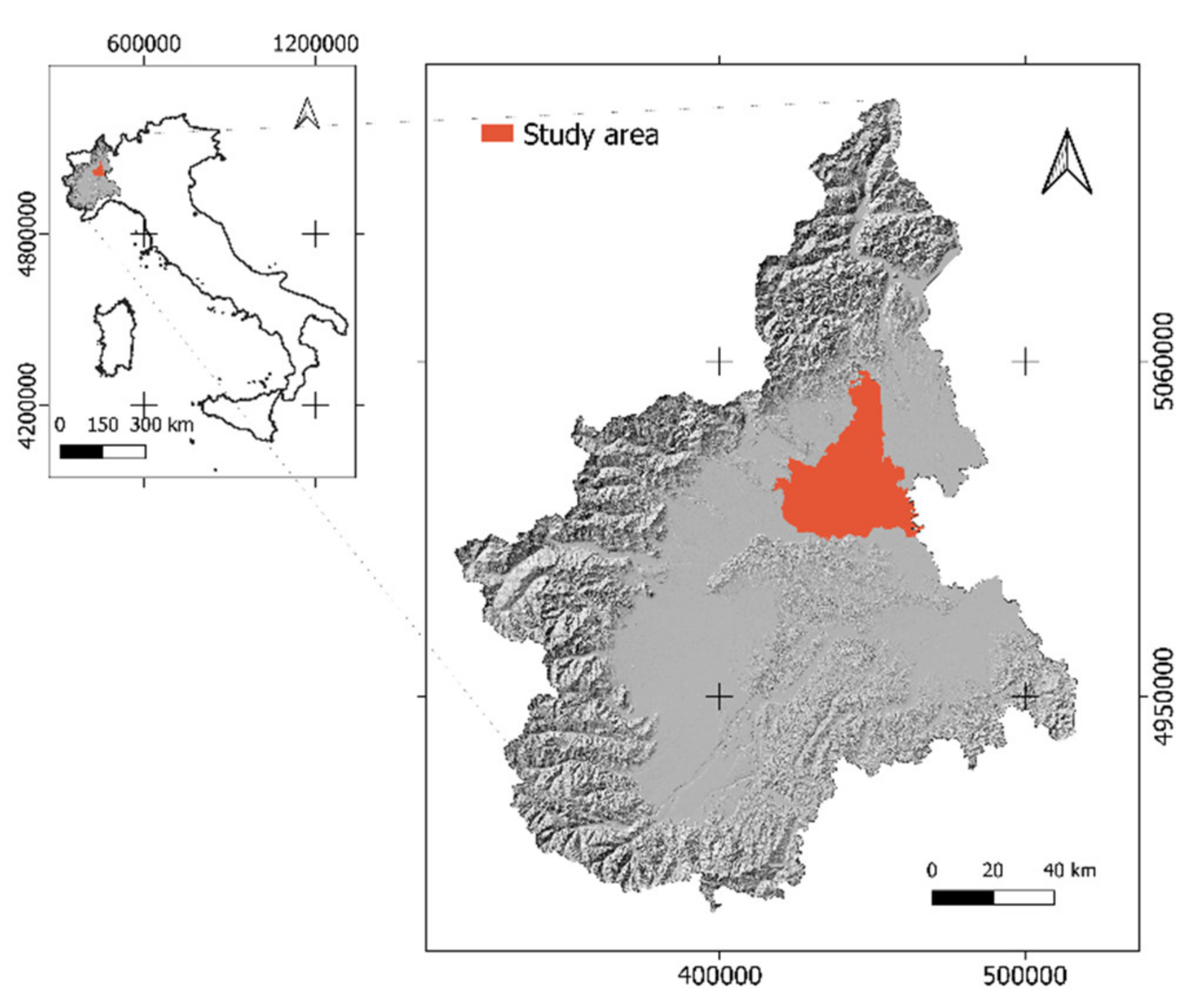
2.1. Study Area
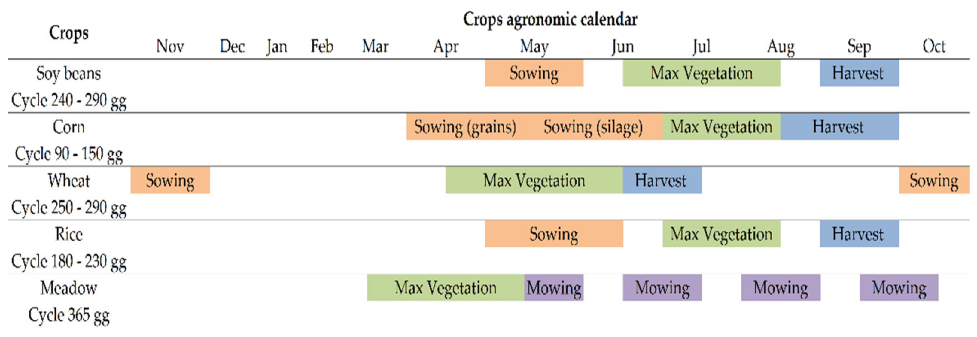
2.2. Crops of Interest
2.3. Copernicus Satellite Data
2.4. Farmers’ GSAA
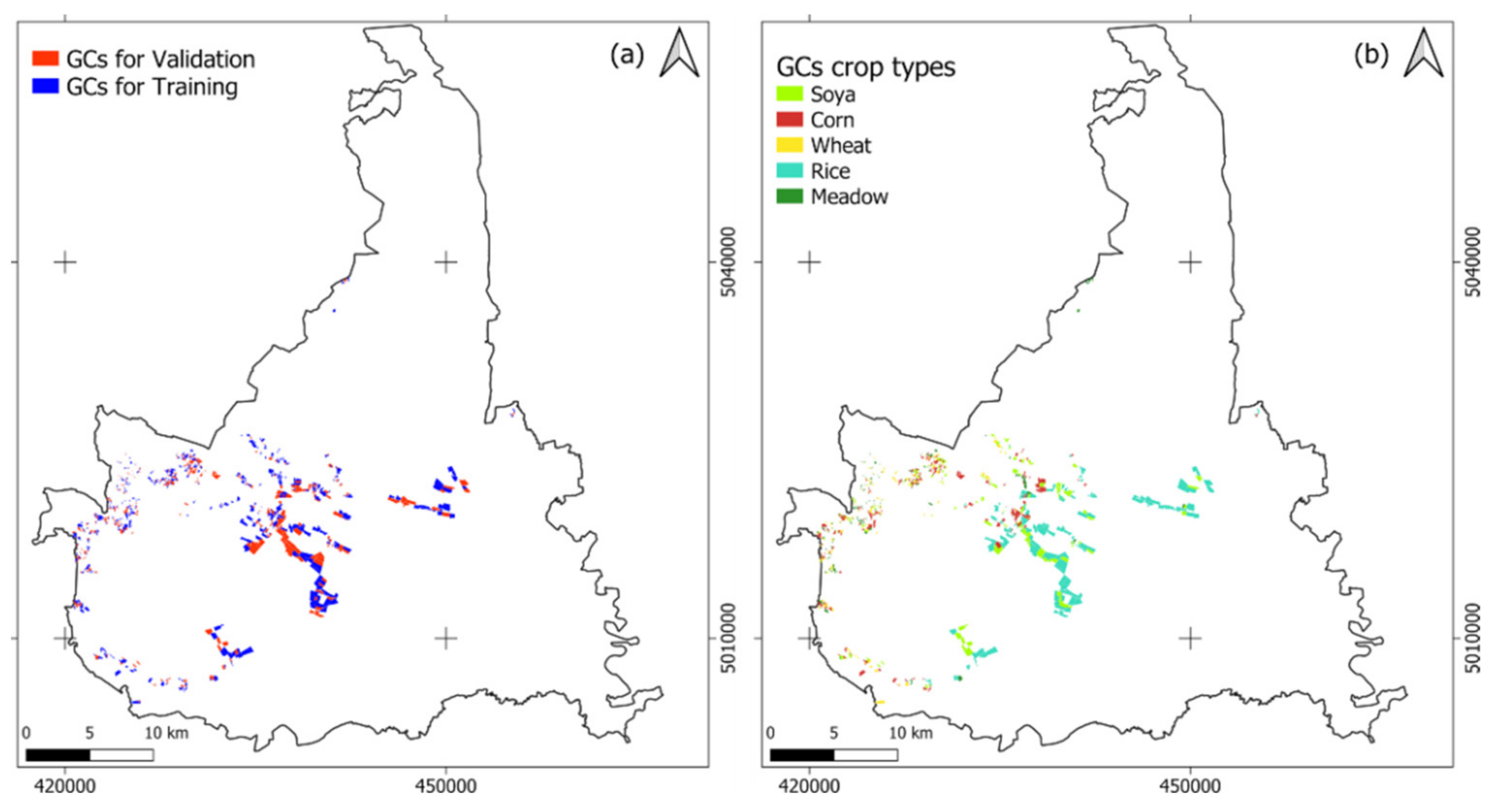
2.5. Ground Data
2.6. Data Processing
2.6.1. Compliance of GSAA with S2 Data
2.6.2. NDVI Image Time Series
2.6.3. Minimum Distance and Random Forest Classification of Crops
2.7. Rule-Based Hierarchical Classification
2.8. Meadow Detection
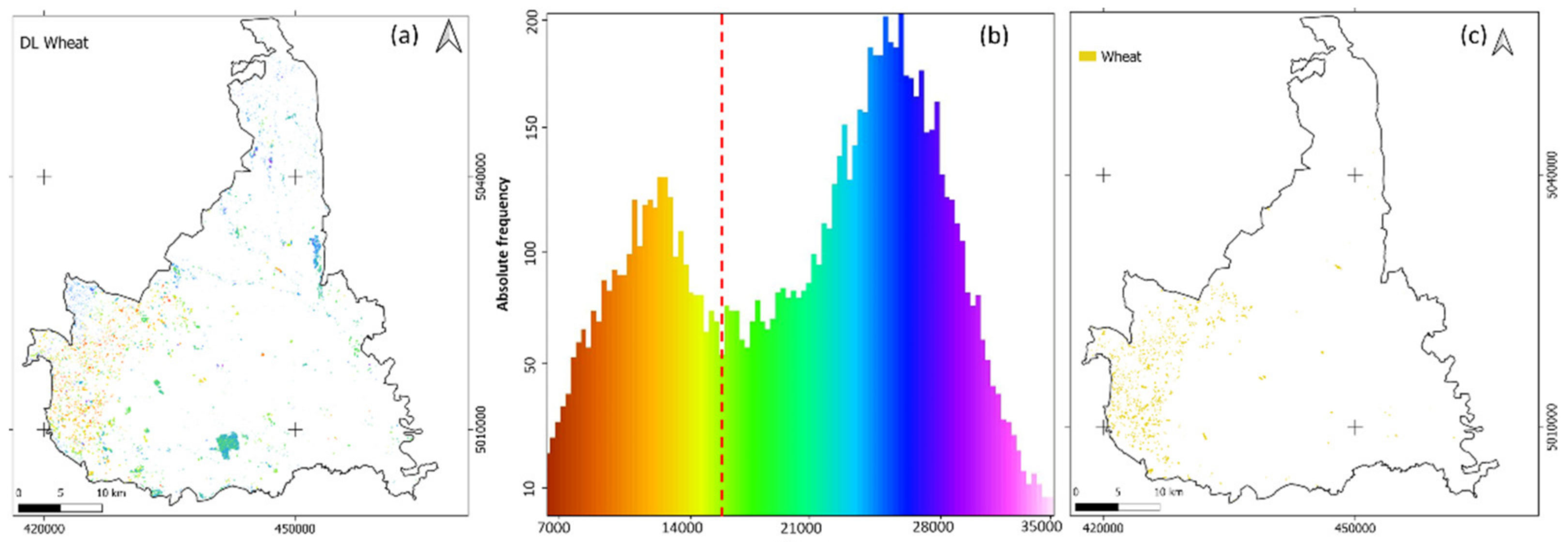
2.9. Wheat Detection
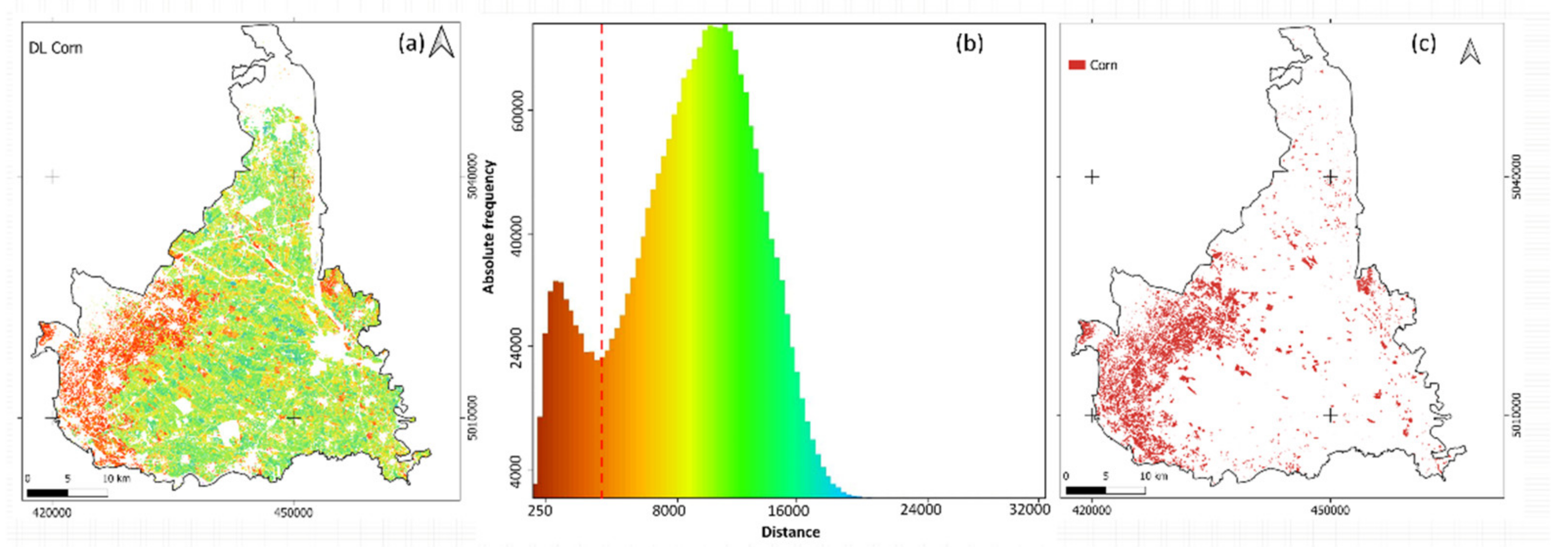
2.10. Corn Detection
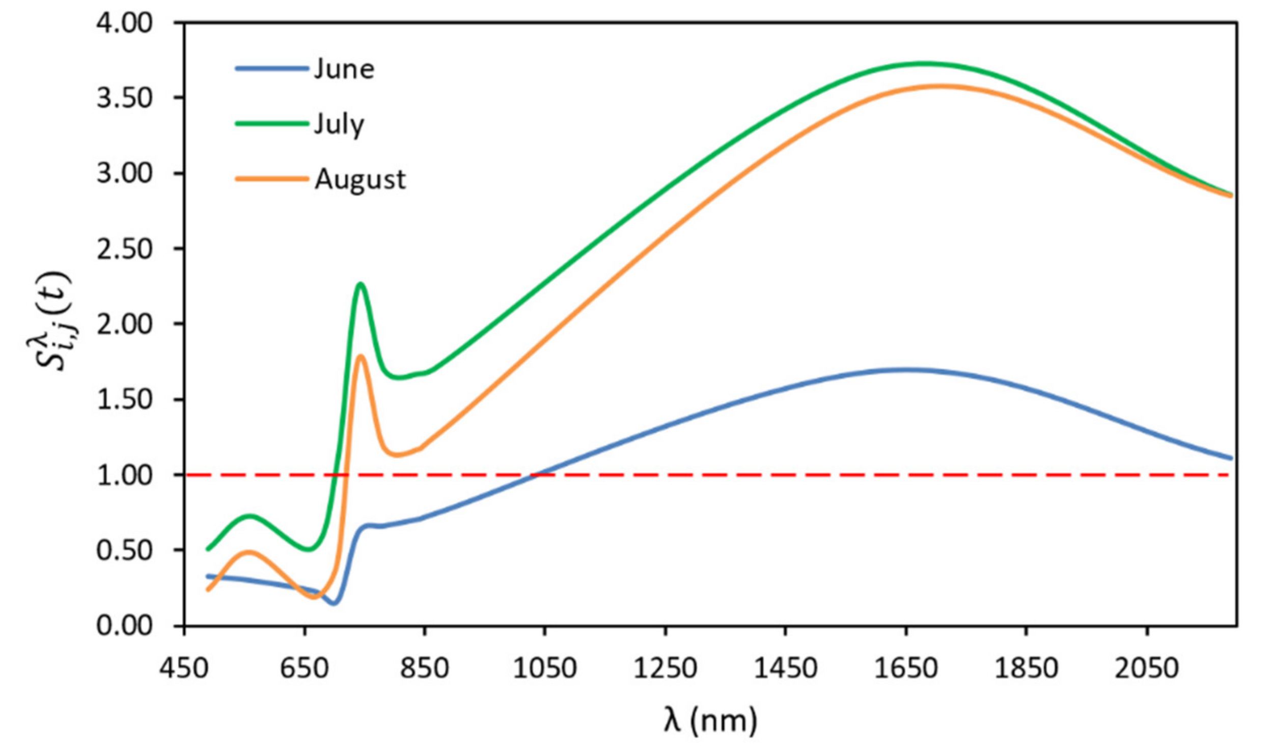
2.11. Soya and Rice Detection
2.12. Comparing HI with MDC and RF
3. Results and Discussion
3.1. Compliance of GSAA Geometry with S2 Data
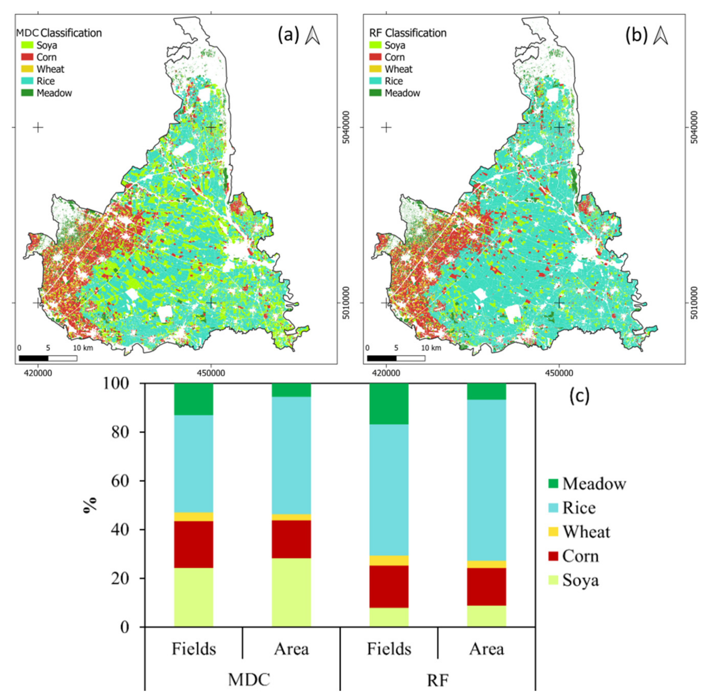
3.2. MDC and RF Classification
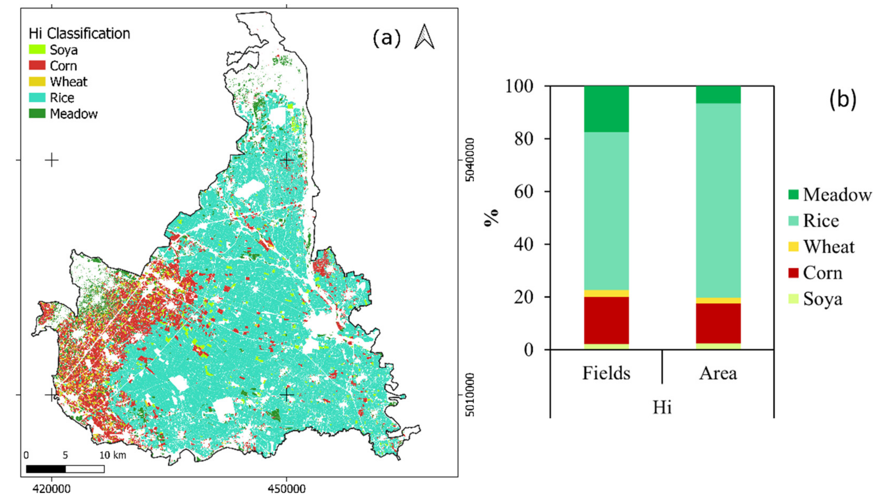
3.3. Rule-Based Hierarchical Classification
3.3.1. Meadow Detection
3.3.2. Wheat Detection
3.3.3. Corn Detection
3.3.4. Soya and Rice Detection
3.4. Comparing HI with MDC and RF
4. Conclusions
Author Contributions
Funding
Data Availability Statement
Acknowledgments
Conflicts of Interest
References
- Geiger, R.; Kotzur, M.; Khan, D.-E. European Union Treaties; Germany Beck: Munich, Germany, 2015. [Google Scholar]
- Dupraz, P.; Guyomard, H. Environment and Climate in the Common Agricultural Policy. EuroChoices 2019, 18, 18–25. [Google Scholar] [CrossRef] [Green Version]
- Shucksmith, M.; Thomson, K.J.; Roberts, D. The CAP and the Regions: The Territorial Impact of the Common Agricultural Policy; CABI Publishing: Wallingford, UK, 2005. [Google Scholar]
- Regulation, C. No 1257/1999 on Rural Development Support by Means of the European Agricultural Guarantee Fund (EAGGF). J. Rural Stud. 1999, 23, 416–429. [Google Scholar]
- Cagliero, R.; Henke, R. Evidence of CAP Support in Italy. Between First and Second Pillar [Common Agricultural Policy]. PAGRI-Politica Agric. Internazionale 2008, 5, 43–62. [Google Scholar]
- Dwyer, J.; Ward, N.; Lowe, P.; Baldock, D. European Rural Development under the Common Agricultural Policy’s ‘Second Pillar’: Institutional Conservatism and Innovation. Reg. Stud. 2007, 41, 873–888. [Google Scholar] [CrossRef]
- Regulation EU No. 809/2014 of the European Parliament and Council with Regard to the Integrated Administration and Control System; Rural Development Measures and Cross Compliance, EU: Maastricht, The Netherlands, 2014; pp. 7272–7286.
- Campinas, M.; Rosa, M.J. Assessing PAC Contribution to the NOM Fouling Control in PAC/UF Systems. Water Res. 2010, 44, 1636–1644. [Google Scholar] [CrossRef]
- Loudjani, P. G-Tech Supports a Common Agriculture Policy in Europe. Geospat. World 2013, 4, 38–40. [Google Scholar]
- Sarvia, F.; Xausa, E.; Petris, S.D.; Cantamessa, G.; Borgogno-Mondino, E. A Possible Role of Copernicus Sentinel-2 Data to Support Common Agricultural Policy Controls in Agriculture. Agronomy 2021, 11, 110. [Google Scholar] [CrossRef]
- Frison, P.-L.; Lardeux, C. Vegetation Cartography from Sentinel-1 Radar Images. QGIS Appl. Agric. For. 2018, 2, 181–213. [Google Scholar]
- Denize, J.; Hubert-Moy, L.; Betbeder, J.; Corgne, S.; Baudry, J.; Pottier, E. Evaluation of Using Sentinel-1 and-2 Time-Series to Identify Winter Land Use in Agricultural Landscapes. Remote Sens. 2018, 11, 37. [Google Scholar] [CrossRef] [Green Version]
- Borgogno-Mondino, E.; Lessio, A.; Gomarasca, M.A. A Fast Operative Method for NDVI Uncertainty Estimation and Its Role in Vegetation Analysis. Eur. J. Remote Sens. 2016, 49, 137–156. [Google Scholar] [CrossRef]
- Segarra, J.; Buchaillot, M.L.; Araus, J.L.; Kefauver, S.C. Remote Sensing for Precision Agriculture: Sentinel-2 Improved Features and Applications. Agronomy 2020, 10, 641. [Google Scholar] [CrossRef]
- Leprieur, C.; Verstraete, M.M.; Pinty, B. Evaluation of the Performance of Various Vegetation Indices to Retrieve Vegetation Cover from AVHRR Data. Remote Sens. Rev. 1994, 10, 265–284. [Google Scholar] [CrossRef]
- Filgueiras, R.; Mantovani, E.C.; Althoff, D.; Fernandes Filho, E.I.; Cunha, F.F. da Crop NDVI Monitoring Based on Sentinel 1. Remote Sens. 2019, 11, 1441. [Google Scholar] [CrossRef] [Green Version]
- Boori, M.S.; Choudhary, K.; Paringer, R.; Sharma, A.K.; Kupriyanov, A.; Corgne, S. Monitoring Crop Phenology Using NDVI Time Series from Sentinel 2 Satellite Data. In Proceedings of the 2019 5th International Conference on Frontiers of Signal Processing (ICFSP), Marseille, France, 18–20 September 2019; IEEE: Piscataway, NJ, USA, 2019; pp. 62–66. [Google Scholar]
- Sarvia, F.; De Petris, S.; Borgogno-Mondino, E. Exploring Climate Change Effects on Vegetation Phenology by MOD13Q1 Data: The Piemonte Region Case Study in the Period 2001–2019. Agronomy 2021, 11, 555. [Google Scholar] [CrossRef]
- Lambert, M.-J.; Traoré, P.C.S.; Blaes, X.; Baret, P.; Defourny, P. Estimating Smallholder Crops Production at Village Level from Sentinel-2 Time Series in Mali’s Cotton Belt. Remote Sens. Environ. 2018, 216, 647–657. [Google Scholar] [CrossRef]
- Sharifi, A. Using Sentinel-2 Data to Predict Nitrogen Uptake in Maize Crop. IEEE J. Sel. Top. Appl. Earth Obs. Remote Sens. 2020, 13, 2656–2662. [Google Scholar] [CrossRef]
- Zhao, Y.; Potgieter, A.B.; Zhang, M.; Wu, B.; Hammer, G.L. Predicting Wheat Yield at the Field Scale by Combining High-Resolution Sentinel-2 Satellite Imagery and Crop Modelling. Remote Sens. 2020, 12, 1024. [Google Scholar] [CrossRef] [Green Version]
- De Petris, S.; Sarvia, F.; Borgogno-Mondino, E. RPAS-Based Photogrammetry to Support Tree Stability Assessment: Longing for Precision Arboriculture. Urban For. Urban Green. 2020, 55, 126862. [Google Scholar] [CrossRef]
- Peters, A.J.; Griffin, S.C.; Viña, A.; Ji, L. Use of Remotely Sensed Data for Assessing Crop Hail Damage. PERS Photogramm. Eng. Remote Sens. 2000, 66, 1349–1355. [Google Scholar]
- Sarvia, F.; De Petris, S.; Borgogno-Mondino, E. Multi-Scale Remote Sensing to Support Insurance Policies in Agriculture: From Mid-Term to Instantaneous Deductions. GISci. Remote Sens. 2020, 57, 770–784. [Google Scholar] [CrossRef]
- Campos-Taberner, M.; García-Haro, F.J.; Martínez, B.; Sánchez-Ruíz, S.; Gilabert, M.A. A Copernicus Sentinel-1 and Sentinel-2 Classification Framework for the 2020+ European Common Agricultural Policy: A Case Study in València (Spain). Agronomy 2019, 9, 556. [Google Scholar] [CrossRef] [Green Version]
- Schmedtmann, J.; Campagnolo, M.L. Reliable Crop Identification with Satellite Imagery in the Context of Common Agriculture Policy Subsidy Control. Remote Sens. 2015, 7, 9325–9346. [Google Scholar] [CrossRef] [Green Version]
- Hao, P.; Zhan, Y.; Wang, L.; Niu, Z.; Shakir, M. Feature Selection of Time Series MODIS Data for Early Crop Classification Using Random Forest: A Case Study in Kansas, USA. Remote Sens. 2015, 7, 5347–5369. [Google Scholar] [CrossRef] [Green Version]
- Lebrini, Y.; Boudhar, A.; Htitiou, A.; Hadria, R.; Lionboui, H.; Bounoua, L.; Benabdelouahab, T. Remote Monitoring of Agricultural Systems Using NDVI Time Series and Machine Learning Methods: A Tool for an Adaptive Agricultural Policy. Arab. J. Geosci. 2020, 13, 796. [Google Scholar] [CrossRef]
- Bannerjee, G.; Sarkar, U.; Das, S.; Ghosh, I. Artificial Intelligence in Agriculture: A Literature Survey. Int. J. Sci. Res. Comput. Sci. Appl. Manag. Stud. 2018, 7, 1–6. [Google Scholar]
- Kim, N.; Ha, K.-J.; Park, N.-W.; Cho, J.; Hong, S.; Lee, Y.-W. A Comparison between Major Artificial Intelligence Models for Crop Yield Prediction: Case Study of the Midwestern United States, 2006–2015. ISPRS Int. J. Geo-Inf. 2019, 8, 240. [Google Scholar] [CrossRef] [Green Version]
- Tian, H.; Huang, N.; Niu, Z.; Qin, Y.; Pei, J.; Wang, J. Mapping Winter Crops in China with Multi-Source Satellite Imagery and Phenology-Based Algorithm. Remote Sens. 2019, 11, 820. [Google Scholar] [CrossRef] [Green Version]
- Veloso, A.; Mermoz, S.; Bouvet, A.; Le Toan, T.; Planells, M.; Dejoux, J.-F.; Ceschia, E. Understanding the Temporal Behavior of Crops Using Sentinel-1 and Sentinel-2-like Data for Agricultural Applications. Remote Sens. Environ. 2017, 199, 415–426. [Google Scholar] [CrossRef]
- Chakhar, A.; Ortega-Terol, D.; Hernández-López, D.; Ballesteros, R.; Ortega, J.F.; Moreno, M.A. Assessing the Accuracy of Multiple Classification Algorithms for Crop Classification Using Landsat-8 and Sentinel-2 Data. Remote Sens. 2020, 12, 1735. [Google Scholar] [CrossRef]
- Sun, R.; Chen, S.; Su, H.; Mi, C.; Jin, N. The Effect of NDVI Time Series Density Derived from Spatiotemporal Fusion of Multisource Remote Sensing Data on Crop Classification Accuracy. ISPRS Int. J. Geo-Inf. 2019, 8, 502. [Google Scholar] [CrossRef] [Green Version]
- Immitzer, M.; Vuolo, F.; Atzberger, C. First Experience with Sentinel-2 Data for Crop and Tree Species Classifications in Central Europe. Remote Sens. 2016, 8, 166. [Google Scholar] [CrossRef]
- Laborte, A.G.; Maunahan, A.A.; Hijmans, R.J. Spectral Signature Generalization and Expansion Can Improve the Accuracy of Satellite Image Classification. PLoS ONE 2010, 5, e10516. [Google Scholar] [CrossRef] [PubMed]
- Rauf, U.; Qureshi, W.S.; Jabbar, H.; Zeb, A.; Mirza, A.; Alanazi, E.; Khan, U.S.; Rashid, N. A New Method for Pixel Classification for Rice Variety Identification Using Spectral and Time Series Data from Sentinel-2 Satellite Imagery. Comput. Electron. Agric. 2022, 193, 106731. [Google Scholar] [CrossRef]
- Boccardo, P.; Mondino, E.B.; Tonolo, F.G. High Resolution Satellite Images Position Accuracy Tests. In Proceedings of the IGARSS 2003 IEEE International Geoscience and Remote Sensing Symposium. Proceedings (IEEE Cat. No. 03CH37477), Toulouse, France, 21–25 July 2003; IEEE: Piscataway, NJ, USA, 2003; Volume 4, pp. 2320–2322. [Google Scholar]
- Delwart, S. SENTINEL-2 User Handbook; European Space Agency: Paris, France, 2015; Available online: https://earth.esa.int/documents (accessed on 14 February 2022).
- Hodgson, M.E. On the Accuracy of Low-Cost Dual-Frequency GNSS Network Receivers and Reference Data. GISci. Remote Sens. 2020, 57, 907–923. [Google Scholar] [CrossRef]
- Xue, J.; Su, B. Significant Remote Sensing Vegetation Indices: A Review of Developments and Applications. J. Sens. 2017, 2017, 1353691. [Google Scholar] [CrossRef] [Green Version]
- Khanal, S.; KC, K.; Fulton, J.P.; Shearer, S.; Ozkan, E. Remote Sensing in Agriculture—Accomplishments, Limitations, and Opportunities. Remote Sens. 2020, 12, 3783. [Google Scholar] [CrossRef]
- Gomarasca, M.A.; Tornato, A.; Spizzichino, D.; Valentini, E.; Taramelli, A.; Satalino, G.; Vincini, M.; Boschetti, M.; Colombo, R.; Rossi, L. Sentinel for Applications in Agriculture. Int. Arch. Photogramm. Remote Sens. Spat. Inf. Sci. 2019, XLII-3/W6, 91–98. [Google Scholar]
- Vajsová, B.; Fasbender, D.; Wirnhardt, C.; Lemajic, S.; Devos, W. Assessing Spatial Limits of Sentinel-2 Data on Arable Crops in the Context of Checks by Monitoring. Remote Sens. 2020, 12, 2195. [Google Scholar] [CrossRef]
- Mondino, E.B.; Corvino, G. Land Tessellation Effects in Mapping Agricultural Areas by Remote Sensing at Field Level. Int. J. Remote Sens. 2019, 40, 7272–7286. [Google Scholar] [CrossRef]
- Conrad, O.; Bechtel, B.; Bock, M.; Dietrich, H.; Fischer, E.; Gerlitz, L.; Wehberg, J.; Wichmann, V.; Böhner, J. System for Automated Geoscientific Analyses (SAGA) v. 2.1. 4. Geosci. Model Dev. 2015, 8, 1991–2007. [Google Scholar] [CrossRef] [Green Version]
- Forman, R.T. Some General Principles of Landscape and Regional Ecology. Landsc. Ecol. 1995, 10, 133–142. [Google Scholar] [CrossRef]
- Rouse, J.W.; Haas, R.H.; Schell, J.A.; Deering, D.W.; Harlan, J.C. Monitoring the Vernal Advancement and Retrogradation (Green Wave Effect) of Natural Vegetation; NASA/GSFC Type III Final Report; US Government Public, Greenbelt, MD, USA, 1974; Volume 371.
- Chen, J.; Jönsson, P.; Tamura, M.; Gu, Z.; Matsushita, B.; Eklundh, L. A Simple Method for Reconstructing a High-Quality NDVI Time-Series Data Set Based on the Savitzky–Golay Filter. Remote Sens. Environ. 2004, 91, 332–344. [Google Scholar] [CrossRef]
- Mishra, A.; Lu, Y.; Meng, J.; Anderson, A.W.; Ding, Z. Unified Framework for Anisotropic Interpolation and Smoothing of Diffusion Tensor Images. NeuroImage 2006, 31, 1525–1535. [Google Scholar] [CrossRef] [PubMed]
- Corvino, G.; Lessio, A.; Borgogno-Mondino, E. Monitoring Rice Crops in Piemonte (Italy): Towards an Operational Service Based on Free Satellite Data. In Proceedings of the IGARSS 2018—2018 IEEE International Geoscience and Remote Sensing Symposium, Valencia, Spain, 22–27 July 2018; IEEE: Piscataway, NJ, USA, 2018; pp. 9070–9073. [Google Scholar]
- Pageot, Y.; Baup, F.; Inglada, J.; Baghdadi, N.; Demarez, V. Detection of Irrigated and Rainfed Crops in Temperate Areas Using Sentinel-1 and Sentinel-2 Time Series. Remote Sens. 2020, 12, 3044. [Google Scholar] [CrossRef]
- Solano-Correa, Y.T.; Bovolo, F.; Bruzzone, L.; Fernández-Prieto, D. Spatio-Temporal Evolution of Crop Fields in Sentinel-2 Satellite Image Time Series. In Proceedings of the 2017 9th International Workshop on the Analysis of Multitemporal Remote Sensing Images (MultiTemp), Brugge, Belgium, 27–29 June 2017; IEEE: Piscataway, NJ, USA, 2017; pp. 1–4. [Google Scholar]
- Akbari, M.; Mamanpoush, A.r.; Gieske, A.; Miranzadeh, M.; Torabi, M.; Salemi, H.R. Crop and Land Cover Classification in Iran Using Landsat 7 Imagery. Int. J. Remote Sens. 2006, 27, 4117–4135. [Google Scholar] [CrossRef]
- Ok, A.O.; Akar, O.; Gungor, O. Evaluation of Random Forest Method for Agricultural Crop Classification. Eur. J. Remote Sens. 2012, 45, 421–432. [Google Scholar] [CrossRef]
- Ustuner, M.; Esetlili, M.T.; Sanli, F.B.; Abdikan, S.; Kurucu, Y. Comparison of Crop Classification Methods for the Sustainable Agriculture Management. J. Environ. Prot. Ecol 2016, 17, 648–655. [Google Scholar]
- Tian, X.; Chen, E.; Li, Z.; Su, Z.B.; Ling, F.; Bai, L.; Wang, F. Comparison of Crop Classification Capabilities of Spaceborne Multi-Parameter SAR Data. In Proceedings of the 2010 IEEE International Geoscience and Remote Sensing Symposium, Honolulu, HI, USA, 25–30 July 2010; IEEE: Piscataway, NJ, USA, 2010; pp. 359–362. [Google Scholar]
- Shi, Y.; Li, J.; Ma, D.; Zhang, T.; Li, Q. Method for Crop Classification Based on Multi-Source Remote Sensing Data. In Proceedings of the IOP Conference Series: Materials Science and Engineering, Wuhan, China, 14–16 June 2019; IOP Publishing: Bristol, UK, 2019; Volume 592, p. 012192. [Google Scholar]
- Zhu, L.; Tateishi, R. Application of Linear Mixture Model to Time Series AVHRR NDVI Data. In Proceedings of the 22nd Asian Conference on Remote Sensing, Singapore, 5–9 November 2001; pp. 5–9. [Google Scholar]
- Wacker, A.G.; Landgrebe, D.A. Minimum Distance Classification in Remote Sensing. LARS Tech. Rep. 1972, 25. [Google Scholar]
- Pal, M. Random Forest Classifier for Remote Sensing Classification. Int. J. Remote Sens. 2005, 26, 217–222. [Google Scholar] [CrossRef]
- Liaw, A.; Wiener, M. Classification and Regression by RandomForest. R News 2002, 2, 18–22. [Google Scholar]
- Kaul, H.A.; Sopan, I. Land Use Land Cover Classification and Change Detection Using High Resolution Temporal Satellite Data. J. Environ. 2012, 1, 146–152. [Google Scholar]
- Kussul, N.; Lavreniuk, M.; Skakun, S.; Shelestov, A. Deep Learning Classification of Land Cover and Crop Types Using Remote Sensing Data. IEEE Geosci. Remote Sens. Lett. 2017, 14, 778–782. [Google Scholar] [CrossRef]
- Nguyen, T.T.; Hoang, T.D.; Pham, M.T.; Vu, T.T.; Nguyen, T.H.; Huynh, Q.-T.; Jo, J. Monitoring Agriculture Areas with Satellite Images and Deep Learning. Appl. Soft Comput. 2020, 95, 106565. [Google Scholar] [CrossRef]
- Lucas, R.; Rowlands, A.; Brown, A.; Keyworth, S.; Bunting, P. Rule-Based Classification of Multi-Temporal Satellite Imagery for Habitat and Agricultural Land Cover Mapping. ISPRS J. Photogramm. Remote Sens. 2007, 62, 165–185. [Google Scholar] [CrossRef]
- Wu, B.; Gommes, R.; Zhang, M.; Zeng, H.; Yan, N.; Zou, W.; Zheng, Y.; Zhang, N.; Chang, S.; Xing, Q. Global Crop Monitoring: A Satellite-Based Hierarchical Approach. Remote Sens. 2015, 7, 3907–3933. [Google Scholar] [CrossRef] [Green Version]
- Kolecka, N.; Ginzler, C.; Pazur, R.; Price, B.; Verburg, P.H. Regional Scale Mapping of Grassland Mowing Frequency with Sentinel-2 Time Series. Remote Sens. 2018, 10, 1221. [Google Scholar] [CrossRef] [Green Version]
- Weber, D.; Schaepman-Strub, G.; Ecker, K. Predicting Habitat Quality of Protected Dry Grasslands Using Landsat NDVI Phenology. Ecol. Indic. 2018, 91, 447–460. [Google Scholar] [CrossRef]
- Sarvia, F.; De Petris, S.; Borgogno-Mondino, E. Mapping Ecological Focus Areas within the EU CAP Controls Framework by Copernicus Sentinel-2 Data. Agronomy 2022, 12, 406. [Google Scholar] [CrossRef]
- De Petris, S.; Squillacioti, G.; Bono, R.; Borgogno-Mondino, E. Geomatics and Epidemiology: Associating Oxidative Stress and Greenness in Urban Areas. Environ. Res. 2021, 197, 110999. [Google Scholar] [CrossRef] [PubMed]
- Otsu, N. A Threshold Selection Method from Gray-Level Histograms. IEEE Trans. Syst. Man Cybern. 1979, 9, 62–66. [Google Scholar] [CrossRef] [Green Version]
- Araújo, G.K.; Rocha, J.V.; Lamparelli, R.A.; Rocha, A.M. Mapping of Summer Crops in the State of Paraná, Brazil, through the 10-Day Spot Vegetation NDVI Composites. Eng. Agrícola 2011, 31, 760–770. [Google Scholar] [CrossRef] [Green Version]
- Hay, A.M. The Derivation of Global Estimates from a Confusion Matrix. Int. J. Remote Sens. 1988, 9, 1395–1398. [Google Scholar] [CrossRef]
- Saganeiti, L.; Pilogallo, A.; Faruolo, G.; Scorza, F.; Murgante, B. Territorial Fragmentation and Renewable Energy Source Plants: Which Relationship? Sustainability 2020, 12, 1828. [Google Scholar] [CrossRef] [Green Version]
- Gascon, F.; Ramoino, F. Sentinel-2 Data Exploitation with ESA’s Sentinel-2 Toolbox. In Proceedings of the EGU General Assembly Conference Abstracts, Vienna, Austria, 23–28 April 2017; p. 19548. [Google Scholar]
- Foerster, S.; Kaden, K.; Foerster, M.; Itzerott, S. Crop Type Mapping Using Spectral–Temporal Profiles and Phenological Information. Comput. Electron. Agric. 2012, 89, 30–40. [Google Scholar] [CrossRef] [Green Version]
- Li, H.; Zhang, C.; Zhang, S.; Ding, X.; Atkinson, P.M. Iterative Deep Learning (IDL) for Agricultural Landscape Classification Using Fine Spatial Resolution Remotely Sensed Imagery. Int. J. Appl. Earth Obs. Geoinf. 2021, 102, 102437. [Google Scholar] [CrossRef]
- Papoutsis, I.; Kontoes, H.; Karathanassi, V.; Koukos, A.; Drivas, T.; Sitokonstantinou, V.; Koutroumpas, A. A Sentinel Based Agriculture Monitoring Scheme for the Control of the CAP and Food Security. Sci. Prepr. 2021, 11524, 1152407. [Google Scholar]
- Beriaux, E.; Jago, A.; Lucau-Danila, C.; Planchon, V.; Defourny, P. Sentinel-1 Time Series for Crop Identification in the Framework of the Future CAP Monitoring. Remote Sens. 2021, 13, 2785. [Google Scholar] [CrossRef]


| MSI Technical Features | SCL Codes | |||
|---|---|---|---|---|
| Geometric Resolution (m) | Bands | Wavelength (nm) | Code | Description |
| 10 | b2 | 458–523 | 0 | No data |
| b3 | 543–578 | 1 | Saturated or defective | |
| b4 | 650–680 | 2 | Dark area pixels | |
| b8 | 785–900 | 3 | Cloud shadows | |
| 20 | b5 | 698–713 | 4 | Vegetation |
| b6 | 733–748 | 5 | Not vegetated | |
| b7 | 773–793 | 6 | Water | |
| b8a | 855–875 | 7 | Unclassified | |
| b11 | 1565–1655 | 8 | Cloud medium probability | |
| b12 | 2100–2280 | 9 | Cloud high probability | |
| 60 | b1 | 433–453 | 10 | Thin cirrus |
| b9 | 935–955 | 11 | Snow | |
| b10 | 1360–1390 | - | - | |
| Crops | Total Number of Surveyed Fields | Total Area of Surveyed Fields (ha) | Training Set (n. Fields) | Training Set (ha) | Validation Set (n. Fields) | Validation Set (ha) |
|---|---|---|---|---|---|---|
| Soya | 220 | 705.2 | 132 (60%) | 393.2 (56%) | 88 (40%) | 312 (44%) |
| Corn | 244 | 493.2 | 146 (60%) | 287 (58%) | 98 (40%) | 206.2 (42%) |
| Wheat | 182 | 246 | 109 (60%) | 167.9 (68%) | 73 (40%) | 78.1 (32%) |
| Rice | 233 | 1554.1 | 140 (60%) | 921.5 (59%) | 93 (40%) | 632.6 (41%) |
| Meadows | 147 | 194.3 | - | - | 147 (100%) | 194.3 (100%) |
| S2 L2A Image | Crop | Phenological Stage |
|---|---|---|
| 15 June 2020 | Soya | Leaf and node development |
| Rice | Tillering | |
| 18 July 2020 | Soya | End node development-bloom |
| Rice | Maximum tiller number-panicle formation | |
| 14 August 2020 | Soya | End bloom-beans develop |
| Rice | Flowering-dough |
| N° of fields before filtering | 196,573 |
| N° of fields after surface filtering | 66,095 |
| N° of fields after geometrical filtering | 57,230 |
| Area of field before filtering (ha) | 97,978 |
| Area of fields after surface filtering (ha) | 95,306 |
| Area of fields after geometrical filtering (ha) | 93,230 |
| Monitorable fields (%) | 29.11% |
| Monitorable area (%) | 95.15% |
Publisher’s Note: MDPI stays neutral with regard to jurisdictional claims in published maps and institutional affiliations. |
© 2022 by the authors. Licensee MDPI, Basel, Switzerland. This article is an open access article distributed under the terms and conditions of the Creative Commons Attribution (CC BY) license (https://creativecommons.org/licenses/by/4.0/).
Share and Cite
Sarvia, F.; De Petris, S.; Ghilardi, F.; Xausa, E.; Cantamessa, G.; Borgogno-Mondino, E. The Importance of Agronomic Knowledge for Crop Detection by Sentinel-2 in the CAP Controls Framework: A Possible Rule-Based Classification Approach. Agronomy 2022, 12, 1228. https://doi.org/10.3390/agronomy12051228
Sarvia F, De Petris S, Ghilardi F, Xausa E, Cantamessa G, Borgogno-Mondino E. The Importance of Agronomic Knowledge for Crop Detection by Sentinel-2 in the CAP Controls Framework: A Possible Rule-Based Classification Approach. Agronomy. 2022; 12(5):1228. https://doi.org/10.3390/agronomy12051228
Chicago/Turabian StyleSarvia, Filippo, Samuele De Petris, Federica Ghilardi, Elena Xausa, Gianluca Cantamessa, and Enrico Borgogno-Mondino. 2022. "The Importance of Agronomic Knowledge for Crop Detection by Sentinel-2 in the CAP Controls Framework: A Possible Rule-Based Classification Approach" Agronomy 12, no. 5: 1228. https://doi.org/10.3390/agronomy12051228
APA StyleSarvia, F., De Petris, S., Ghilardi, F., Xausa, E., Cantamessa, G., & Borgogno-Mondino, E. (2022). The Importance of Agronomic Knowledge for Crop Detection by Sentinel-2 in the CAP Controls Framework: A Possible Rule-Based Classification Approach. Agronomy, 12(5), 1228. https://doi.org/10.3390/agronomy12051228