Article

An Agricultural Event Prediction Framework towards Anticipatory Scheduling of Robot Fleets: General Concepts and Case Studies

1
Faculty of Science and Technology, Norwegian University of Life Sciences (NMBU), 1430 Aas, Norway
2
Lincoln Centre for Autonomous Systems (LCAS), University of Lincoln, Lincoln LN6 7TS, UK
*
Author to whom correspondence should be addressed.
Agronomy 2022, 12(6), 1299; https://doi.org/10.3390/agronomy12061299
Submission received: 13 March 2022 / Revised: 4 May 2022 / Accepted: 9 May 2022 / Published: 29 May 2022

Abstract

:
Harvesting in soft-fruit farms is labor intensive, time consuming and is severely affected by scarcity of skilled labors. Among several activities during soft-fruit harvesting, human pickers take 20–30% of overall operation time into the logistics activities. Such an unproductive time, for example, can be reduced by optimally deploying a fleet of agricultural robots and schedule them by anticipating the human activity behaviour (state) during harvesting. In this paper, we propose a framework for spatio-temporal prediction of human pickers’ activities while they are picking fruits in agriculture fields. Here we exploit temporal patterns of picking operation and 2D discrete points, called topological nodes, as spatial constraints imposed by the agricultural environment. Both information are used in the prediction framework in combination with a variant of the Hidden Markov Model (HMM) algorithm to create two modules. The proposed methodology is validated with two test cases. In Test Case 1, the first module selects an optimal temporal model called as picking_state_progression model that uses temporal features of a picker state (event) to statistically evaluate an adequate number of intra-states also called sub-states. In Test Case 2, the second module uses the outcome from the optimal temporal model in the subsequent spatial model called node_transition model and performs “spatio-temporal predictions” of the picker’s movement while the picker is in a particular state. The Discrete Event Simulation (DES) framework, a proven agricultural multi-robot logistics model, is used to simulate the different picking operation scenarios with and without our proposed prediction framework and the results are then statistically compared to each other. Our prediction framework can reduce the so-called unproductive logistics time in a fully manual harvesting process by about 80 percent in the overall picking operation. This research also indicates that the different rates of picking operations involve different numbers of sub-states, and these sub-states are associated with different trends considered in spatio-temporal predictions.

1. Introduction

Precision agriculture concept is based on information-intensive agriculture, prescription farming and identification of suitable tools to minimize cost through enhanced productivity while simultaneously conserving the resources [1]. Nowadays, cost-effective intelligent systems based on automation and robotics technologies are needed for improved performance in agricultural fields. Such cutting-edge solutions must also be inherently safe and reliable for human and environment [2,3]. Harvesting operations in agricultural farms are not only about safely picking up the crop yields but also about optimal resource management and operational logistics planning. These concerns are more critical in soft-fruit farms, as the short-shelf life of the fruits, that requires transportation of picked fruits to a cold storage facility as soon as possible. During picking operations, human pickers spend around 20–30% of the overall working time just in logistics activities such as transportation and unloading, where they walk with trays of picked fruits and empties by moving back and forth from the crop to the storage location [4,5]. Shortage of skilled farm workers is another major difficulty faced by many commercial soft-fruit growers around the world, resulting in fruits left unpicked, especially during worst-case scenarios like economic crisis and pandemic [6].
Though farming systems employ large-sized machines like tractors, nearly 10% of the field area is used for operating these machines for logistics operations [7]. Hence, the usage of small size robots, or even a fleet of them, has an advantage over conventional farm vehicles for better utilization of the agricultural land area. Moreover, modular autonomous robots such as the Thorvald platform can be easily reconfigured for different in-field tasks and do not demand for any special arrangements [8].
An initial Wizard-of-Oz (WoZ) study in [9] was conducted with the Thorvald robot in a real strawberry farm in the presence of human pickers (Figure 1), to check the advantages that a robot brings to workers during harvesting. The authors evaluated how an autonomous robot for in-field transportation system would assist fruit pickers and what benefits this solution could provide to the production process. The in-field transportation is still an open problem for the production of various fruit crops (e.g., strawberries, raspberries, apples), which demand the deployment of sustainable management approaches for robot fleets in real field applications [10]. Optimal management of multi-robot systems is the key idea to reduce operating time of harvesting and, thus, deploying these robots based on spatio-temporal predictions of harvesting events would improve efficiency of the human pickers and eventually benefit the farmers.
The conceptual idea of using a fleet of coordinated vehicles for agricultural tasks is not a novelty. Many research groups are developing fleet management systems for dealing with task management, motion planning, traffic control, data analysis, and fleet monitoring (e.g., battery levels, mission status, robots locations and so on). In [11] the authors discuss some hardware architectures for robot fleets to improve reliability, lower development costs, and allow software integration from different developers. Three different hardware topologies for fleets of robots were introduced to reduce the computing system to a minimum: central-external controller, central-internal controller and immerse controller. In [12], the authors address the design, development, testing and assessment of a new generation of heterogeneous robot fleets (ground and aerial), equipped with innovative sensors, enhanced end-effectors, and improved decision-making algorithms for effective weed and pest management in the crop fields. A novel augmented reality system is proposed in [13] to help farmers supervise the operation of autonomous agricultural machinery towards efficient fleet management and safe operation based on situational awareness. A cloud-based in-field fleet coordination system for multiple sequential operations on large-scale farms is introduced in [14], wherein the authors developed a collaborative self-driving operating system for fleet management using a strip-state updating algorithm for successive field operations under an optimal strategy for conditioning the waiting time between sequential operations. Following this trend, fleets of autonomous robots designed to monitor plants, eliminate weeds and harvest crops with human awareness can definitely become commercially available in the coming years.

1.1. Problem Formulation

The main motivation for this work comes from the RASberry project, a.k.a. Robotics and Autonomous Systems for Berry Production, that aims to develop an autonomous fleet of robots operating in human-assisting environments for agricultural farms of strawberry production [7]. The tasks available in the field are shared among the fleet of robots which are governed by a central coordination system to ensure an optimized task distribution across the entire fleet. To optimize the number of robots in a fleet and their workflow, the fleet coordination component must learn how to anticipate human worker needs and optimize the spatial distribution of robots available for a picker. According to [4], autonomous robots were provided “on-demand” of pickers for in-field logistics. They have used an online mobile-based application to request, cancel or to get the status of a particular transportation robot. We suspect that the “on-demand” policy in in-field logistics is prone to human errors with inability to use digital devices, or waste in time for pickers while waiting for robot to reach to them. To overcome this, a key idea for an improvement in in-field logistics is shown in Figure 2, that emphasizes sending a robot to the picker’s location by “anticipating-demand” instead of “on-demand” while they are in picking operation. This solution aims to get rid of the portable digital device and is also capable of reducing the pickers’ waiting time for a robot.

1.2. Related Works

Deploying fleet of robots is a cutting-edge solution, which is predominant in warehouse industries [15] but with still few applications in agriculture [16]. Much of the existing works in agri-robotics mostly address problems of path planning, and goal assignment of multiple robots and farm vehicles [17,18], with a few use cases on human-robot assistance.
Agriculture is not a money driven industry, which means it also asks for productivity gain on each cost invested in the implementation of robots on the field [2]. Indeed, different regions have distinct field characteristics, and infrastructure. Under such a dynamic environment, a faster analysis tool would help in exploration of different processes and operation in in-field logistics before actually deploying the robots. In this context, the Discrete Event Simulation (DES) framework is adopted from [4], to model the picking scenarios in presence of soft-fruit human pickers and fleet of robots and validating our prediction framework.
Spatio-temporal predictions in agricultural fields are discussed mainly for crop management and yield estimation [19,20,21]. Still, there is not much concern regarding the modeling of the human picker’s motion in constrained agricultural environments. In a recent work [22], the authors have developed a prediction approach for localising and tracking human pickers inside polytunnels using a novel Topological Particle Filter (TPF) algorithm. However, this solution is still limited to “on-demand” calling a robot for transport assistance. Our proposed prediction framework is working towards the automatic calling of the robot by “anticipating-demand”.
According to [23], machine learning-based methods were applied for human motion prediction integrated with video data or used for other forecasting applications. However, such methods have a few common pitfalls such as hyper-parameter tuning, depth and complexity of the models. Recently, there is a growing interest in dynamic object motion prediction based on Bayesian approaches for efficient human-robot collaboration [24,25], combined with optimal motion planning and collision-free trajectory generation for mobile robots [26,27].
Hidden Markov Models (HMMs) [28], a particular case of Bayesian network, are attractive for the modeling of the state progression [29]. However, conventional HMMs has the limitation of dealing with irregularly sampled continuous-time data such as in our case of picking operation performed by human pickers. Based on proven research on similar type of data in medical applications of diseases progression [30,31,32], human and vehicle motion prediction [33], and human-motion recognition [34], we propose the use of a Continuous-time HMM (CtHMM) for the spatio-temporal prediction framework for different picking scenarios.

1.3. Our Proposal and Contribution
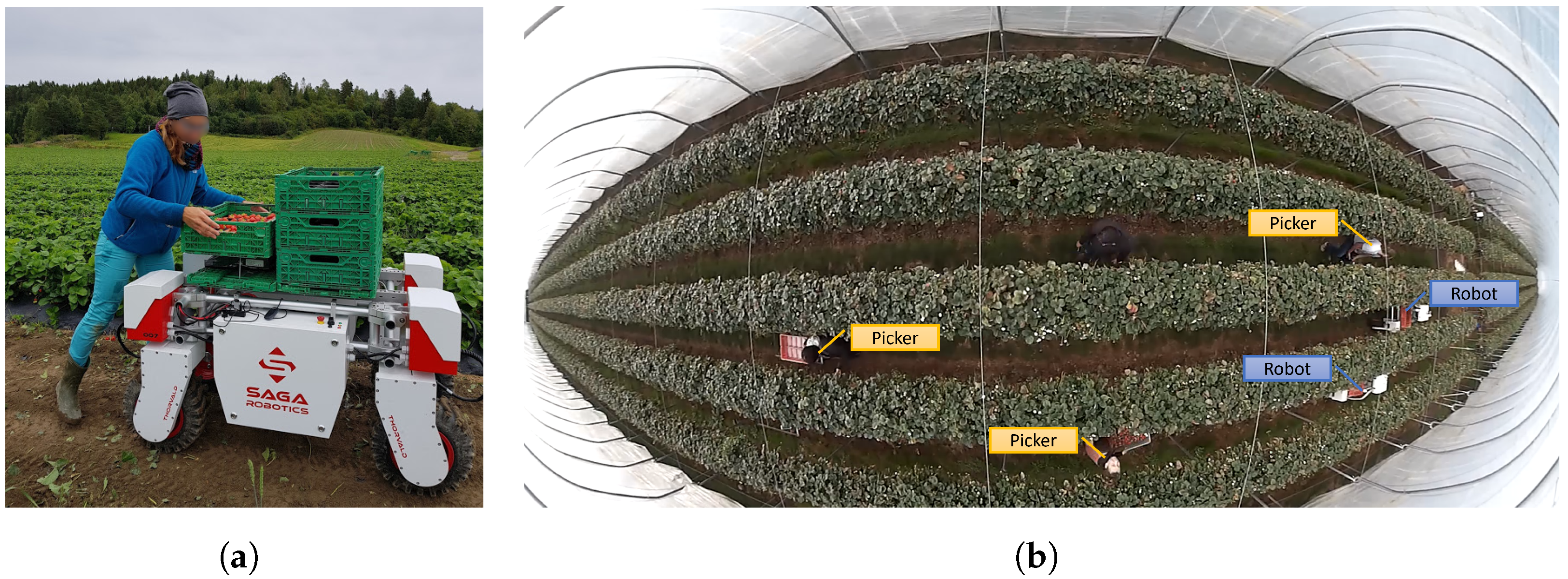
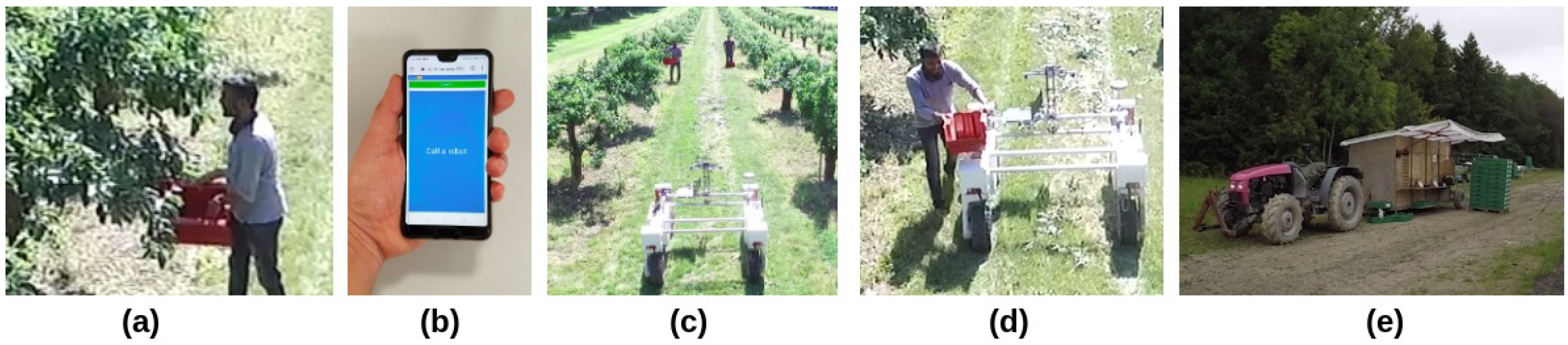
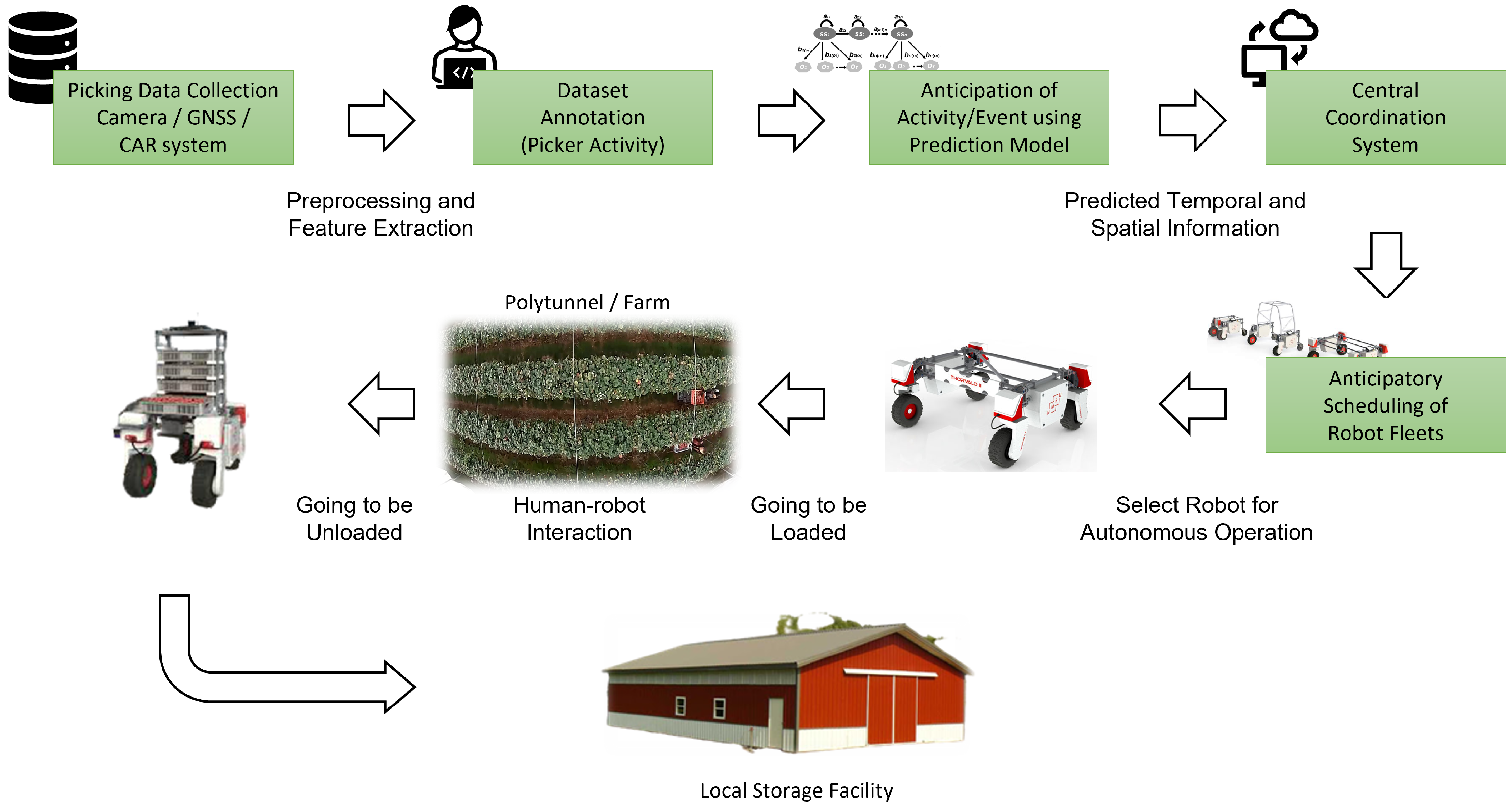
The proposed spatio-temporal prediction framework consists of two prediction models: one is called picking_state_progression model and other is called node_transition model. The former predicts the temporal dynamics of harvesting activities (tray_full_time) and the latter predicts the spatial dynamics for individual pickers (tray_full_node). The validation of the prediction framework is carried out by using the DES framework [4] fed with data from real harvesting operations. Then, two test cases are considered: in Test Case 1, we have the picking_state_progression model working for a given average picking_time to observe how efficiently a temporal progression of a state can be predicted, without loosing too much of information over a period of time. In Test Case 2, the temporal prediction outcome obtained from the picking_state_progression model and the mean_picking_rate are given as input in the node_transition model, to predict picker’s location in a 2D discretized topological map of the agricultural field. The relation between the picking_time and mean_picking_rate is given as follows: the picking_time for a “tray-full event” is equal to the topological node-to-node distance divided by the mean_picking_rate multiplied by the farm yield.
In this work, our main contributions are as follows: (i) develop a spatio-temporal prediction framework of the picker activity status by exploiting the constrained 2D discrete map information of the environment called topological map and using statistical learning methods. This model should investigate the possible progression of a state and accordingly making anytime prediction of the location of the pickers; (ii) based on simulations with real-field data through case studies, we have also analyzed the feasibility of our prediction models in reducing unproductive time such as, transportation time or waiting time of human pickers during picking operation along the crop fields.
This paper is organized as follows: in Section 2, we present the system overview, followed by a brief discussion on the topological map and a state abstraction for the picking operation. Section 3 presents the proposed spatio-temporal prediction framework, the states of the individual CtHMMs and the predictions obtained from the CtHMMs; in Section 4, we introduce the experimental evaluation and the analysis of the simulation results for two case studies; Section 5 finally presents the concluding remarks and perspectives for future works.

2. System Overview

In this section, an overview of the whole field picking operation for the RASberry use case and some of the necessary tools to achieve this goal are reported, which are needed to better understand the evaluation of the results.

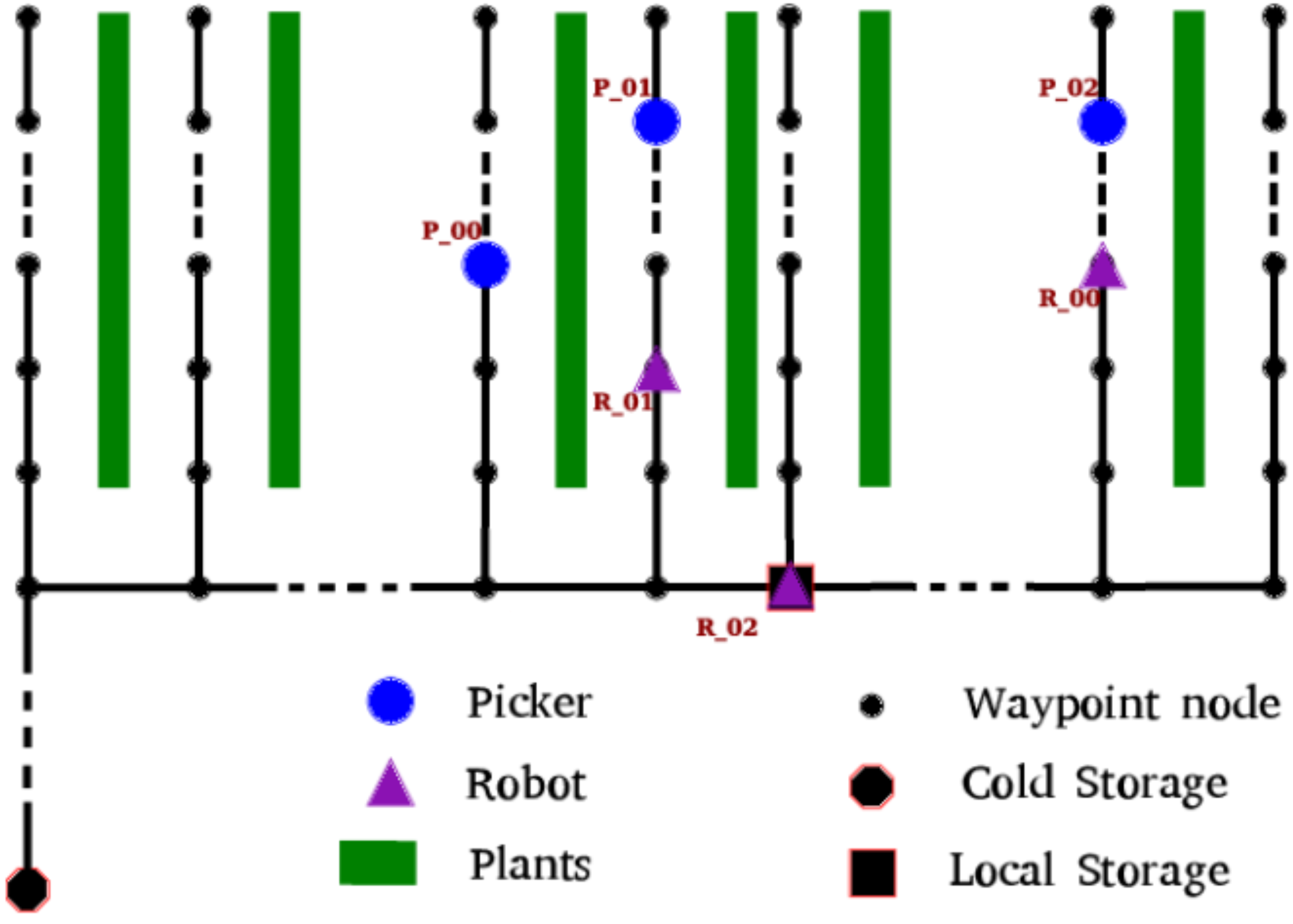
2.1. The Topological Map

In the DES framework, the agricultural field is discretized into a 2D topological map [35], which is a graph of discrete points located in a 2D space called as topological nodes. A general representation of the topological map is shown in Figure 3, where a topological node is denoted as a waypoint node. According to [36], it provides a unified system that can tackle different challenges in terms of continuous navigation of autonomous robot in agriculture field. It can be described as a tuple T = N , E , A , n a v , where N is a set of physical location points { n 1 , n 2 , , n κ } , κ is the total number of locations, and E N × N shows the set of possible edges connecting the nodes element i-th row and j-th column of E, defined as:
E i j = 1 , if n i connects to n j , 0 , elsewhere .
The navigation from one topological node to another is possible only if an edge exists between them. Here, A is the set of actions performed by robots to navigate by mapping of each edge to navigation action, n a v . The picking process is discretized by looking at the changes in the picker activities while moving from one topological node to another.

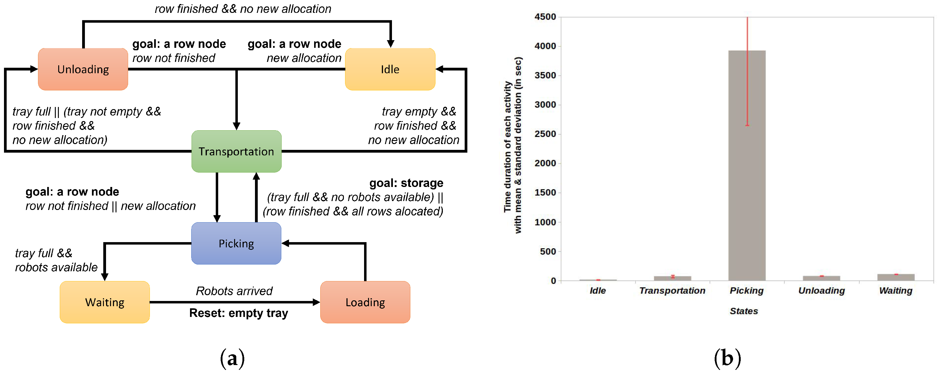
2.2. A State Abstraction for Picking Operation

To better understand the distinct states of human pickers in a real-time fruit picking operation, below we discuss manual and robot-assisted picking operation procedures. The picking operation protocols are almost similar for different fruit picking environment such as strawberry polytunnels or apple orchards. The operation is described as follows: at the outset of picking operation, a group of human pickers are assigned to a certain row of an agriculture farm. They will start picking fruits in tray by moving forward or backward (i.e., ascending or descending order respectively, of topological map node IDs) in a given crop row. When a tray is full (called a “tray-full event”), in manual operation Figure 4, they themselves will transport and unload the tray by moving to the local storage. However, in robot-assisted operation Figure 5, they will push a button interface of an in-house app called CAR (Call-A-Robot) system on a mobile device and wait for the robot to come to nearby location [22]. Then, the pickers get the service in transportation and unloading of the fruit tray(s). In both cases, after finishing unloading the tray, they resume picking again from the last position they were picking, or in a new row if the previous row is finished. This cycle of events repeats until the harvesting tasks is completed for all crop rows in the field. For the sake of simplicity, we have assumed that the robot speed and the transportation speed of the human picker are the same.
The bottleneck problem in both manual and robot-assisted picking operations is that the pickers have to spend significant time on unproductive activities, either transporting trays or waiting for the robot to arrive respectively. Reducing the time of unproductive activities forms the basis for the evaluation of our proposed anticipatory scheduling framework.

Categorizing the Picker’s States

According to [4], we have categorised pickers activities into six states from the real-time data observations in RASberry use-case picking operation as Idle, Transportation, Picking, Unloading, Loading, and Waiting, as shown in Figure 6a. Among all states, Picking (or picking state) is found to be the dominant one which depicts the time duration of a “tray-full event” (or tray_full_time) and all other states are highly dependent on it. Thus, in this work, we are concerned with modeling picking_state_progression for prediction. An example of time duration of each picker’s state is shown in Figure 6b.

3. A Topological Map-Based Spatio-Temporal Prediction Framework

This section presents the proposed spatio-temporal prediction framework for the RASberry use case, discussing the details of the individual CtHMMs and the system architecture processes for “tray-full events” predictions used in our test case studies.

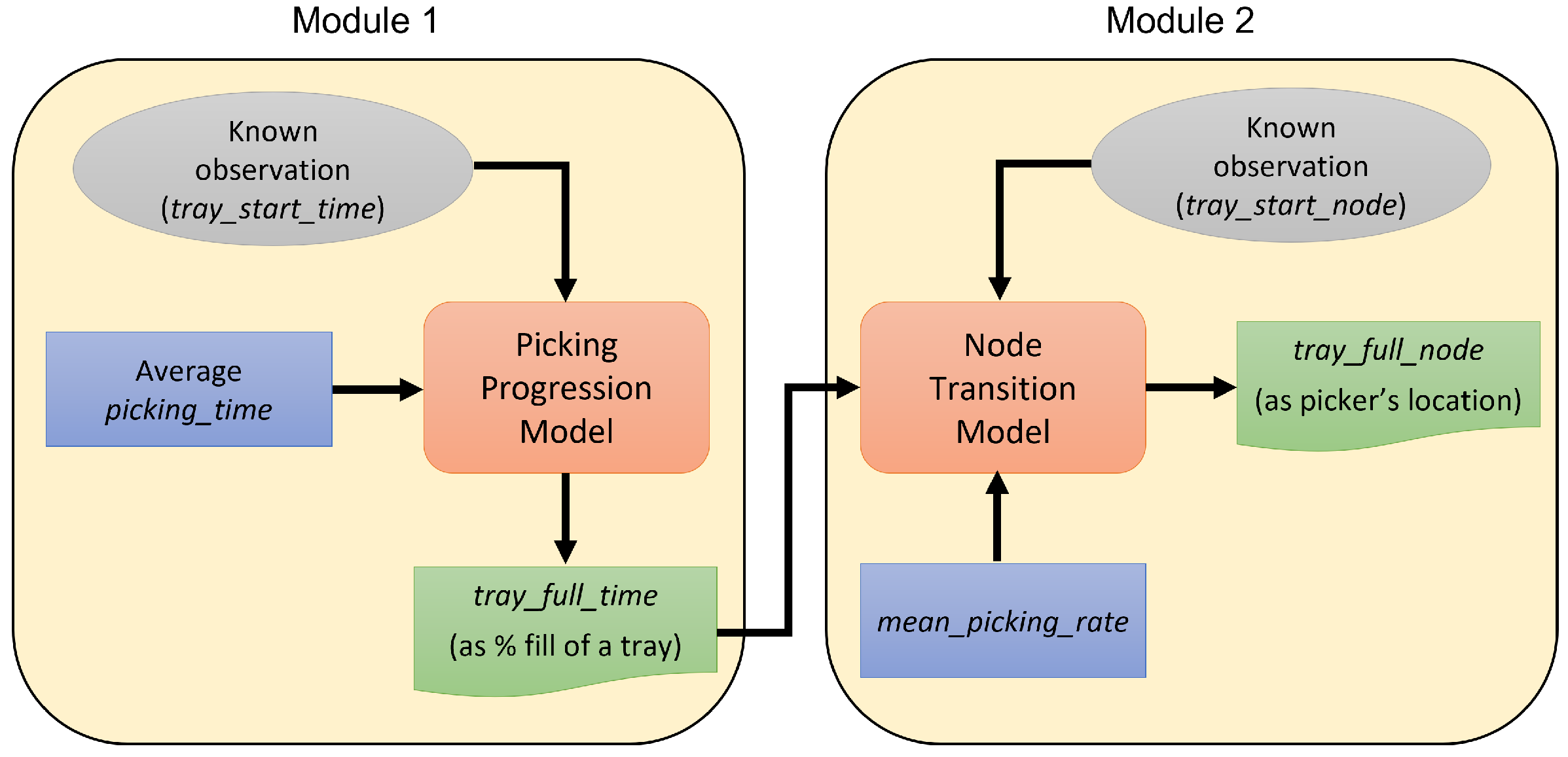
3.1. Spatio-Temporal Prediction Modules

As shown in Figure 7, our prediction framework consists of two modules each with a particular CtHMM. The first module comprises the picking_state_progression model, which outputs the expected time of filling up of a tray as well as predicts temporal progression with respect to percent filling of a tray, for a given average picking_time as input. Here, we assume that every state (e.g., the picking state) is associated with a probability of transition to another state, which is a function of state duration and resets to zero once a transition to another state occurs. Therefore, without loss of generality, we consider that the picking_state_progression as an exponential function defined by the mean of resident time in a state. Being a dominant state, it has high chances of self-transition for input picking_time. Then, the picking_time is discretized into several segments called sub-states. The sub-states imply that the state of picker will exhibit the same behavior for a certain period. Then, each sub-state signifies the percentage of the tray that is full at a given time in the future. These achieved sub-states correspond to “hidden states” of the picker. Later, we will determine the number of such sub-states required in the spatial prediction model using a statistical model evaluation method.
The second module comprises the node_transition model, which predicts topological node location for input temporal progression of a tray and mean_picking_rate. The node_transition model is a spatial prediction model created by exploiting the discrete nodes of the topological map of a given agricultural field into a CtHMM and using it to predict the picker location at any time in the future. In the next section, we will explain in detail both individual CtHMMs.

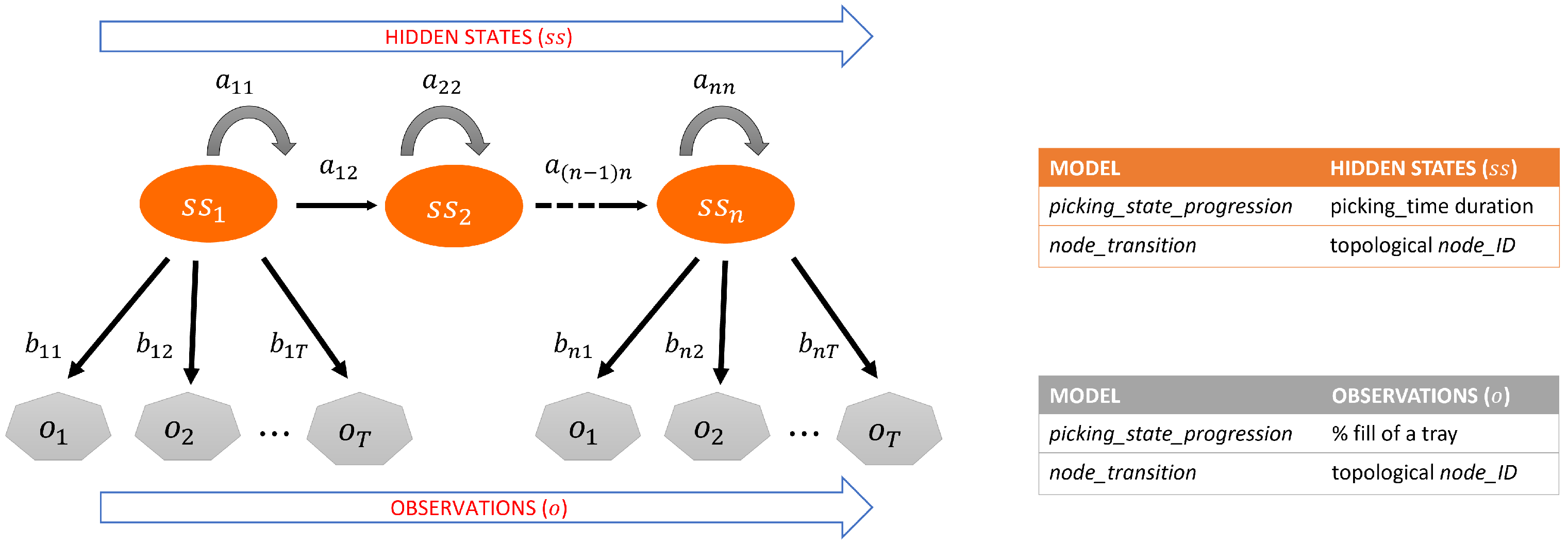
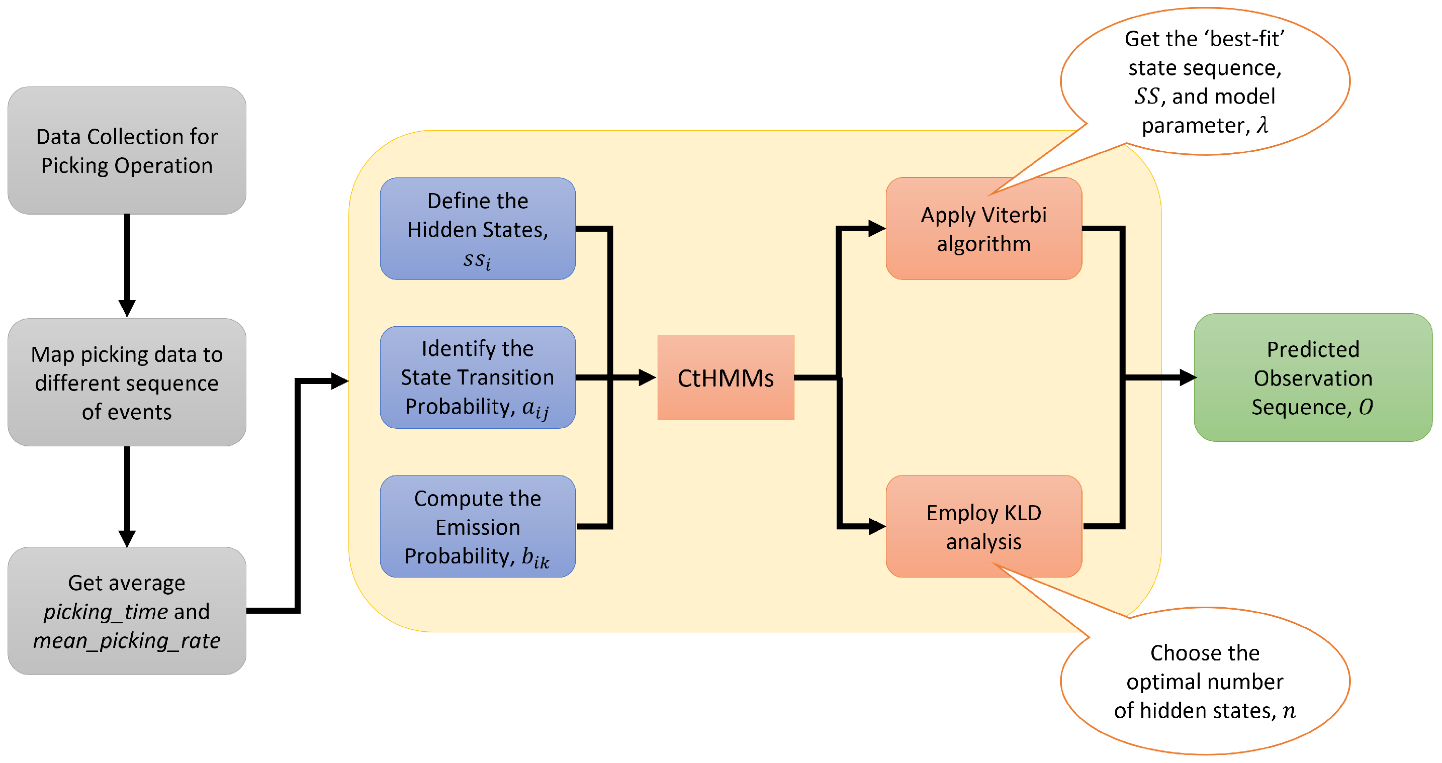
3.2. Design of Individual CtHMMs

Each CtHMM model represents the sequence of observed feature vectors corresponding to each hidden state, considering an emission probability. A graphical representation of a general model state transition is shown in Figure 8. A CtHMM can be represented as a tuple λ = S S , A , π , O , B for state transition at each unit of time t [37]. These parameters for our models are defined in what follows: SS is the set of hidden states S S = { s s 1 , s s 2 , , s s n } and n is the number of states in the hidden state sequence. For the picking_state_progression model, s s i S S is the i-th sub-state within the picking operation starting from an empty tray and ending with a “tray-full event”, which is equivalent to a fixed progression of filling a tray. In the node_transition model, these hidden states are the topological nodes in the environment (node_ID), representing the spatial position of the picker. The initial state or prior probability vector π R 1 × n is given by:
π i = P ( s s i ) , i = 1 , , n ,
which determines in which state s s i the picking process begins. A R n × n is the state transition matrix where its entries a i j provide the transition probability from state s s i to state s s j as:
a i j = P ( s s j | s s i ) , s s i , s s j S S ,
where the state transition coefficients satisfy
a i j 0 , i , j = 1 , , n , and Σ j = 1 n ( a i j ) = 1 , s s i S S .
Here, O is the set of observable states O = { o 1 , o 2 , , o T } or observations, where T is the number of samples in the observed response sequence. For the picking_state_progression model, o k O is the k-th observation (emission) within the picking operation, which is equivalent to the percentage of picking progress and denoted by x. In the node_transition model, these observable states are the topological node location denoted by node_ID. For every hidden state, B R n × ( n + 1 ) is an output observation distribution whose entries b i k provide the emission probability as:
b i k = P ( o k | s s i ) , o k O , s s i S S .

3.3. Predictions from the CtHMMs

The overall processes involved in the prediction from either of the CtHMM are shown in Figure 9. In this case study, data from the harvesting operation of a commercial strawberry production field were collected from devices such as cameras, Garmin GNSS receiver, and CAR system [22]. The data from all the sensors were processed to extract the timestamps of each picker activity. For example, we have visually inspected and fetched the time duration of a tray full event by tracking each picker in the video manually. Similarly, we have processed GNSS timestamps as well as CAR system timestamps to classify different picker activities. More details about the CAR system can be found in [22]. After that, temporal features were extracted and mapped to different picker’s state (see Figure 6a). Next, the average picking_time for a tray and the mean_picking_rate are fed into the CtHMM for picking_state_progression and node_transition models respectively. The parameters of the CtHMM are calculated using the aforementioned Equations (2)–(5). From our proposed architecture, the objective is to predict “when” and “where” a picker would fill a complete tray with respect to the topological node location, given the observations of the picker’s current picking progress.
Since the sub-state driven models are nearly nested, it is expected that the more complex model with higher number of hidden states would have larger posterior likelihood, and at least a good fit, as the simple model. However, the main questions that arise when we apply CtHMM are: (i) how to enquire the certainty of the state posterior distribution of the observation sequences from different sub-state models and accordingly choose an optimal model with suitable number of hidden states? And (ii) how to get the `best-fit’ hidden state sequence S S = { s s 1 , s s 2 , , s s n } of the given observation sequence O = { o 1 , o 2 , , o T } and parameters of the sub-state model λ ?
The first problem is solved using the Kullback–Leibler divergence (KLD) method as being suitable for model comparison in the Bayesian framework, that intuitively measures how much a given arbitrary distribution is away from the true distribution [38]. Basically, it computes the information loss in the fitted model relative to that in the reference model and is denoted as:
K L ( p | | q ) = p ( x ) · ln ( p ( x ) / q ( x ) ) d x otherwise , if p 0 , q = 0 .
where p ( x ) is represents the “true” distribution of data (observation) and q ( x ) represents the approximation (model) of p ( x ) . In this paper, KLD is compared against uniform distribution q ( x ) , which is defined as a 1-D array of n samples with an equal probability of 1 / n . Apparently, the model with minimum KLD index is considered as the optimal choice. However, in this paper, the threshold KLD index is set close to 1 for a model with a given sub-state size and picking operation time interval, to be considered a good fit. In other words, a simpler model with less number of sub-states is compromised with a complex model with more number of sub-states only if the KLD value is found within range 1 ± 0.05. The second problem is solved by using the Viterbi algorithm which is based on the maximum likelihood estimation (MLE) [39]. Next, we will present two case studies and their corresponding experimental analysis.

4. Experimental Evaluation

In this section, we present the experimental evaluation to demonstrate the effectiveness and feasibility of the proposed prediction framework. We have carried out multiple DES trials with prediction models running on the Ubuntu 16.04 LTS operating system based-workstation with Intel® CoreTM i7-7500U CPU and 16 GB RAM. Our DES framework follows the picking protocols from the RASberry use case for picking operation, as discussed in Section 2.2. The DES framework codes were written in Python, enabling easy integration with the Robot Operating System (ROS) framework [40]. The DES trials with/without prediction framework have adopted and initialized the field variables, according to the DES framework explained in [4], as follows: normalized farm yield as 0.0650 ± 0.0013 crates per discrete node distance, picker’s normalized picking_rate and transportation_rate as 0.0375 ± 0.0007 ms−1 and 1.00 ± 0.02 ms−1 respectively. In our experiments, we are using 6 rows of an open rectangular field of strawberry plants, each row 120 m long and separated by 1.5 m with equidistant topological node-to-node distance of 5 m. The resulting topology (see Figure 3) of the site corresponds to a comb pattern with the main transportation route containing the local store connecting starting points of all rows. On average, the simulations reported in this work took approximately 13–15 min to simulate all the events of roughly 2 : 30 h clock time.
Our CtHMM-based prediction framework predicts the next “tray-full event” for each of the pickers not only based on field conditions, but also based on their individual conditions (e.g., tray start node, time and picking directions, pickers having a break, and so on). These predictions are made periodically to incorporate any changes in the conditions of individual pickers. For example, after each picker completes a “tray-full event” in the field, the mean_picking_rate and average picking_time for that tray are calculated from their tray_start_node, tray_start_time, tray_full_node and tray_full_time, and are used to have a better mean rate to be used for future predictions. The actual tray_full_node and tray_full_time are obtained from the CAR system which is used by the picker to call for a robot in regular operations and as a monitoring system when robots are allocated based on the predictions. The experimental tests were carried out and the analysis of the results are presented in the following subsections.

4.1. Test Case 1: To Choose an Optimal Picking_State_Progression Model

We will first explain in details the parameters chosen for the picking_state_progression model and then, in the later part, we show the analysis of the experiment outcome. In this experiment. we want to get the optimal number of hidden states (sub-states) for a given picking_time in order to achieve an optimal model.
Accordingly, the picking_time is divided into n sub-states where each sub-state means 100/n % of a “tray-full event” occurrence. Once picker is in picking state, he/she would be in such a state till a tray is finished, which means the sub-state transition always happens in forward direction. Since the tray filling is naturally progressive, the given sub-state transition probability in the model, denoted by the state transition matrix A, is cyclic, having an extremely low probability in the reverse direction.
The output observation distribution B is set for the prediction model such that each sub-state has 70 % of probability to emit itself as an observation, another 10 % for each neighbouring sub-state and 0.1 % for all observations, to ensure numerical stability. We also include 10 % change for occurrence of “unknown” noisy observation, which each node is equally likely to emit in prediction. The initial state probability π is set uniformly as 1/n, for each hidden state (sub-state).
To validate our picking_state_progression model, several runs on DES framework were executed considering different number of sub-states. First, we start with a random sub-state size of 5, and the corresponding graph results for each test run with sub-state size incremented up to 30 are plotted in Figure 10. Then, the goodness of the fit to the data is checked using the Viterbi algorithm. The log-likelihood distribution is then inferred using KLD analysis. For the sake of simplicity and practical aspects, we have only considered few situations to demonstrate the KLD analysis. According to Figure 10 and from the results shown in Table 1, for a picker’s mean_picking_rate equal to 0.0375 ms−1 and the prediction time interval 9, the KLD value for the prediction model with number of sub-states 30 was found to be closer to the true distribution than in other cases.

4.2. Test Case 2: Spatio-Temporal Predictions of the Picker’s Motion

Based on the results obtained from Test Case 1, a picking_state_progression model with 30 substates is combined with node_transition model to make the complete “tray-full event” prediction in Test Case 2. Here, it is assumed that the picker is following the picking protocol (see Section 2.2). The CtHMM parameters (A, π , B) used in this model are calculated as the same way as in Test Case 1.
To check the accuracy of the predictions, the DES framework was run with both CtHMMs and analyzed against the actual data obtained from the DES running based on the manual picking operation, with two pickers. The prediction results were evaluated with respect to the occurrence of a “tray-full event” for a single picker and the overall picking operation with multiple pickers, to understand the feasibility of using an anticipatory scheduling strategy. In this work, our focus is on reducing the time consumption in logistics operations based on the human picker’s activities predictions, although the DES trials are executed with robots equal to the number of pickers in each farm row, as shown in Figure 3. However, the explicit evaluation of an optimal number of robots required to assist the human pickers in the field, the task allocation, and the concerns regarding the scheduling of robots are out of the scope of this work for now.
Here, for the sake of better understanding, we will adopt the acronyms mentioned in detail in Table 2: t r a y _ f u l l _ t i m e (TFT); p r e d i c t i o n _ t i m e _ e r r o r (PTE); t r a n s p o r t a t i o n _ t i m e per tray (TTT); number of average nodes covered per “tray-full event” (ANCT); Node transition time (NTT); average “tray-full event” time (ATT); average process completion time (APCT); save on transportation time (STT); frequency of occurrence (FoO); percentage average error (PAE).

4.2.1. Analysis for a Single Picker

As mentioned previously, this analysis is needed for a specific CtHMM model with mean_picking_rate, and it would keep providing the same results for the same picking start node and time. Otherwise, different CtHMM models can be created for different pickers based on their picking dynamics or changes in field dynamics (say, changes in node-to-node space), resulting in changes in “tray-full event” prediction (and consequently PTE) as well. As shown in Table 3, it is observed that a picker with an Id 00 starts picking at 1.9 s in forward direction from row_ID 00 and node_ID 00. Then, Tray 1 is anticipated to finish in 2096.7 s, but actually it takes 2114.9 s with same number of covered nodes, 16, and so on. Similarly to the real appointed nodes row_IDs, the picker is predicted to cover 3 rows (row_ID 00, 02, 04) and to finish 7 full trays in total completion time of 15,680.1 s whereas in actual it takes 15,686.2 s. The predicted forward (F) and reverse (R) directions for picking trays are found to be same as the actual data. However, in few cases of the predicted “tray-full event” (e.g., Tray No. 2, 3, 6), the node_IDs are found to be deviated by ± 1 node from the actual tray full node location of a picker. If the predicted node is ahead of actual node, for example Tray No. 2 and 3, the PTE per tray is always found negative. Such a value came up as a result of an extra prediction time used to cover one extra node. Otherwise, when the predicted node is equal to (or less than) the actual node, PTE gives mostly positive value, except for a few cases (e.g., Tray 4). It is worth mentioning that reducing the distance between adjacent topological nodes from 5 m (say, 2.5 m) can also reduce this negative PTE.
In our case, as a convention, when applying an anticipatory scheduling strategy with robots, a negative value of PTE is called as picker_waiting_time for the robot (e.g., Tray No. 2, 3, 4), whereas a positive value is called as robot_waiting_time (e.g., Tray No. 1, 5, 6, 7) for the picker. It is worth noticing that, we are concerned in this work only for saving the picker_waiting_time and not the robot_waiting_time. However, for deploying an optimized anticipatory scheduling of the robot fleets for human pickers both waiting times need to be considered in a next work.
The predicted results for human-robot interaction based on an anticipatory scheduling are evaluated, as shown in Table 4. These results show us how much probable STT can be achieved, according to the predicted node_ID for a “tray-full event” and PTE. Then, four main prediction classes were observed. In Class 1, a robot can be sent to the actual current node of a picker and wait till he/she finishes a tray. Then, the picker can unload to the robot without even travelling much distance with a filled tray. In Class 2, the picker might need to travel just about one node (i.e., about 5 m) to unload, and can save on transportation time by avoid travelling all the way to the local storage. In Class 3 and Class 4, the picker will be waiting for a short period of time, till a robot reaches to the picker’s current node location. This waiting time would be extremely small (e.g., PTE of Tray 4) in comparison to the average TTT.
Considering the transportation speed 1.0 ± 0.02 ms−1 for a picker, as discussed earlier, the TTT is calculated as approximately 121.57 ± 13.39 s to unload 7 trays. Hence, for all classes, % STT per tray is obtained by using the following relation:
STT ( % ) = TTT PTE TTT × 100 .
In Class 3, a robot is predicted to be sent to a node located ahead the actual picker location (e.g., Tray 2, 3). Then, a robot can not obviously pass the picker, but it needs to stop at the picker’s current tray full node. The PTE value in such classes consists of an “offset” of an extra predicted Node Transition Time (NTT). Here, NTT is defined as “how much time a picker takes to move from one node to its subsequent node while picking”, being calculated as:
NTT = TFT ANCT .
When removing the NTT from PTE it will provide us the PTE value (picker_waiting_time or robot_waiting_time) for the predicted node which should be the same as the picker’s actual “tray-full event” node. The actual NTT and predicted NTT are normally distributed as 146.57 ± 5.70 s and 129.22 ± 7.28 s respectively. Thus, for a particular situation like Tray 2, PTE is found as 25.2 s instead of 154.5 s. However, for such classes in general, picker_waiting_time is normally distributed as 17.35 ± 2.23 s. Correspondingly, considering the situation where a predicted node is either the same as or ahead of picker’s actual tray full node, % STT per tray is calculated by using Equation (7), as approximately 85.72 ± 0.37 %.

4.2.2. Analysis for an Overall Picking Operation

According to the prediction analysis shown in Table 5, for the overall picking process of 7 tray full events with two pickers, the predicted APCT were 15,787.85 ± 142.48 s. On average, this value is 0.38 % more than the actual APCT, which is 15,726.02 ± 56.28 s. The increase in the predicted APCT was expected as a result of the randomly distributed picking and transportation rates. Based on the “tray-full event” analysis of the whole process, the predicted ANCT by an average picker to fill a tray is approximately 16.07 ± 0.82 with an ATT normally distributed as 2255.26 ± 26.78 s. On the contrary, in actual, ATT is approximately 2246.57 ± 11.37 s and ANCT is approximately 15.78 ± 0.80 . Hence, based on the PAE value of the overall process, the predicted picking process is approximately 0.38 ± 1.09 % slower than the actual picking process. In addition, the predicted process shows an “offset” node coverage of approximately 1.8 ± 0.10 % , which means 0.28 ± 0.03 number of nodes more than the actual number of nodes to fill a tray.
Based on the predicted and actual values of ATT, the PTE value is calculated as picker_waiting_time of 8 s with a little deviation of 24.64 s. Hence, this ensures that the PTE value is falling into an acceptable category of Class 1, 2, or 4, where either picker has to wait at the “tray-full event” node for a while or travel a few meters of distance, in order to unload a tray. Accordingly, based on the estimated values of TTT and PTE for the overall process, the % STT is calculated by using Equation (7), as approximately 79.74 ± 9.70 . Additionally, considering the safety of the picker while interacting with robot under an anticipatory scheduling strategy, the error in node prediction is found within the acceptable range.
It is worth mentioning that the current pilot study is conducted to check the feasibility of the proposed prediction framework for fruit picking operations. It is also intended to create a baseline prediction model against manual picking operation. Here, running the DES framework for manual operation implies that the robots are included and sent to the picker’s location as/when they call for a robot. Conversely, running the DES framework with CtHMMs implies that the robots are included and sent to the picker’s location in advance by anticipating the requirement of the robot during the picking operation. Future research work will focus on implementing autonomous robot-assisted picking operations, with and without an anticipatory scheduling framework. Furthermore, the DES framework can be extended to include a fleet of robots with a high number of pickers in the operation. Please see [4] for allocating logistics tasks to a fleet of robots. It is noteworthy that our prediction framework can be easily extended to a large number of human pickers. We can also group pickers with similar picking rates together and use a single model for making predictions for each of them.

5. Conclusions and Perspectives

In this work, we have presented a preliminary study for developing the anticipatory scheduling of robots in the agricultural field to assist human pickers in various operations. The utilization of the DES framework allows the systematic analysis of different picking scenarios based on predictions. Based on our simulation results for an individual picker, at each “tray-full event”, the prediction methodology has depicted four classes, with respect to the predicted and actual node location in the topological map. Three classes (1, 2 and 4) have proved to be favorable for the anticipatory scheduling when the expected node is located ahead or at the same node as the actual node of the picker.
Spatial and temporal predictions using two CtHMMs have been shown to be quite effective with small error in operating time of approximately 0.38 % greater than in the actual case for the overall picking process. An average picker is predicted to cover just 0.28 ± 0.03 number of extra nodes to fill a tray picking in similar direction as that of the actual case. Another advantage of this study is that scheduling a robot based on our prediction model may reduce the transportation time approximately by 79.74 ± 9.70 % , on overall picking operation. In our case studies on real-world farms, it was observed that the pickers hardly ever take a break until the harvesting operation is completed, and this is not considered in the evaluations. Even if a picker takes a break from the harvesting operation, due to the periodic predictions being made with our spatial-temporal prediction framework, predictions for the individual pickers who are taking a break can be removed from this particular round of predictions. We believe that reducing transportation time can improve the utilization of human pickers in agricultural fields and help reduce their physical strain.
The main outcomes of this work are quite promising and allow us to glimpse future applications of such an event prediction framework for human-robot collaboration in manufacturing and autonomous driving in urban environments. In the future, the focus would be to implement our prediction model in different agricultural fields to analyze the effectiveness of the anticipatory scheduling strategy in real-time and real-world scenarios. Further extending this work, we intend to improve our prediction framework, including other picker states such as Idle, Transportation, Loading, and Unloading.

Author Contributions

Conceptualization, G.D., M.H. and A.P.; methodology, A.P. and G.D.; software, G.D., A.P. and M.H.; formal analysis, A.P. and G.D.; resources, A.P. and G.D.; writing—original draft preparation, A.P., G.D. and A.C.L.; writing—review and editing, G.D., A.C.L., M.H. and P.J.F.; supervision, A.C.L., P.J.F. and M.H. All authors have read and agreed to the published version of the manuscript.

Funding

This research was partially supported by the RASberry funding programme (https://rasberryproject.com/ (accessed on 12 March 2022)) and UK Research and Innovation within the scope of Innovate UK Robot Highways, project reference InnovateUK 51367.

Institutional Review Board Statement

Not applicable.

Informed Consent Statement

Informed consent was obtained from all subjects involved in the study.

Data Availability Statement

The data presented in this study are available on request from the corresponding author.

Acknowledgments

We would like to thank Jon G. O. Gjevestad for all valuable comments and suggestions, which were taken into consideration to improve the overall quality and readability of the manuscript.

Conflicts of Interest

The authors declare no conflict of interest.

References

  1. Srinivasan, A. (Ed.) Handbook of Precision Agriculture: Principles and Applications; Food Products Press, An Imprint of the Haworth Press, Inc.: Binghamton, NY, USA, 2006. [Google Scholar]
  2. Bechar, A.; Vigneault, C. Agricultural Robots for Field Operations: Concepts and Components. Biosyst. Eng. 2016, 149, 94–111. [Google Scholar] [CrossRef]
  3. Vasconez, J.P.; Kantor, G.A.; Auat Cheein, F.A. Human-robot Interaction in Agriculture: A Survey and Current Challenges. Biosyst. Eng. 2019, 179, 35–48. [Google Scholar] [CrossRef]
  4. Das, G.; Cielniak, G.; From, P.; Hanheide, M. Discrete Event Simulations for Scalability Analysis of Robotic in-Field Logistics in Agriculture—A Case Study. In Proceedings of the IEEE International Conference on Robotics and Automation, Workshop on Robotic Vision and Action in Agriculture, Brisbane, Australia, 21–26 May 2018; pp. 1–6. [Google Scholar]
  5. Achillas, C.; Bochtis, D.; Aidonis, D.; Marinoudi, V.; Folinas, D. Voice-driven Fleet Management System for Agricultural Operations. Inf. Process. Agric. 2019, 6, 471–478. [Google Scholar] [CrossRef]
  6. Bochtis, D.; Benos, L.; Lampridi, M.; Marinoudi, V.; Pearson, S.; Sørensen, C.G. Agricultural Workforce Crisis in Light of the COVID-19 Pandemic. Sustainability 2020, 12, 8212. [Google Scholar] [CrossRef]
  7. From, P.J.; Grimstad, L.; Hanheide, M.; Pearson, S.; Cielniak, G. Rasberry—Robotic and Autonomous Systems for Berry Production. ASME Mech. Eng. 2018, 140, S14–S18. [Google Scholar] [CrossRef] [Green Version]
  8. Grimstad, L.; From, P. The Thorvald II Agricultural Robotic System. Robotics 2017, 6, 24. [Google Scholar] [CrossRef] [Green Version]
  9. Baxter, P.; Cielniak, G.; Hanheide, M.; From, P. Safe Human-Robot Interaction in Agriculture. In Proceedings of the Companion of the 2018 ACM/IEEE International Conference on Human-Robot Interaction, Chicago, IL, USA, 5–8 March 2018; pp. 59–60. [Google Scholar]
  10. Sørensen, C.; Bochtis, D. Conceptual Model of Fleet Management in Agriculture. Biosyst. Eng. 2010, 105, 41–50. [Google Scholar] [CrossRef]
  11. Emmi, L.; Gonzalez-de Soto, M.; Gonzalez-de Santos, P. Configuring a Fleet of Ground Robots for Agricultural Tasks. In ROBOT2013: First Iberian Robotics Conference: Advances in Robotics; Armada, M.A., Sanfeliu, A., Ferre, M., Eds.; Springer International Publishing: Cham, Switzerland, 2014; pp. 505–517. [Google Scholar]
  12. de Santos, P.G.; Ribeiro, A.; Fernandez-Quintanilla, C.; Lopez-Granados, F.; Brandstoetter, M.; Tomic, S.; Pedrazzi, S.; Peruzzi, A.; Pajares, G.; Kaplanis, G.; et al. Fleets of Robots for Environmentally-safe Pest Control in Agriculture. Precis. Agric. 2017, 18, 574–614. [Google Scholar] [CrossRef]
  13. Huuskonen, J.; Oksanen, T. Augmented Reality for Supervising Multirobot System in Agricultural Field Operation. In Proceedings of the 6th IFAC Conference on Sensing, Control and Automation Technologies for Agriculture, Sydney, Australia, 4–6 December 2019; pp. 367–372. [Google Scholar]
  14. Wu, C.; Chen, Z.; Wang, D.; Song, B.; Liang, Y.; Yang, L.; Bochtis, D.D. A Cloud-Based in-field Fleet Coordination System for Multiple Operations. Energies 2020, 13, 775. [Google Scholar] [CrossRef] [Green Version]
  15. Wurman, P.R.; D’Andrea, R.; Mountz, M. Coordinating Hundreds of Cooperative, Autonomous Vehicles in Warehouses. AI Mag. 2008, 29, 9–20. [Google Scholar]
  16. Ball, D.; Ross, P.; English, A.; Milani, P.; Richards, D.; Bate, A.; Upcroft, B.; Wyeth, G.; Corke, P. Farm Workers of the Future: Vision-Based Robotics for Broad-Acre Agriculture. IEEE Robot. Autom. Mag. 2017, 24, 97–107. [Google Scholar] [CrossRef]
  17. Bochtis, D.; Sørensen, C.; Vougioukas, S. Path Planning for In-field Navigation-aiding of Service Units. Comput. Electron. Agric. 2010, 74, 80–90. [Google Scholar] [CrossRef]
  18. Conesa-Muñoz, J.; Bengochea-Guevara, J.M.; Andujar, D.; Ribeiro, A. Efficient Distribution of a Fleet of Heterogeneous Vehicles in Agriculture: A Practical Approach to Multi-path Planning. In Proceedings of the IEEE International Conference on Autonomous Robot Systems and Competitions, Vila Real, Portugal, 8–10 April 2015; pp. 56–61. [Google Scholar]
  19. Xu, W.; Wang, Q.; Chen, R. Spatio-temporal Prediction of Crop Disease Severity for Agricultural Emergency Management based on Recurrent Neural Networks. GeoInformatica 2018, 22, 363–381. [Google Scholar] [CrossRef]
  20. Ozaki, V.A.; Ghosh, S.K.; Goodwin, B.K.; Shirota, R. Spatio-temporal Modeling of Agricultural Yield Data with an Application to Pricing Crop Insurance Contracts. Am. J. Agric. Econ. 2008, 90, 951–961. [Google Scholar] [CrossRef] [PubMed] [Green Version]
  21. Tokovenko, O.; Dorfman, J.H.; Gunter, L.F. A Spatio-temporal Model for Agricultural Yield Prediction. In Proceedings of the Annual Meeting: Agricultural and Applied Economics Association, Denver, CO, USA, 25–27 July 2010; pp. 1–17. [Google Scholar]
  22. Khan, M.W.; Das, G.P.; Hanheide, M.; Cielniak, G. Incorporating Spatial Constraints into a Bayesian Tracking Framework for Improved Localisation in Agricultural Environments. In Proceedings of the IEEE/RSJ International Conference on Intelligent Robots and Systems, Las Vegas, NV, USA, 25–29 October 2020; pp. 2440–2445. [Google Scholar]
  23. Martinez, J.; Black, M.J.; Romero, J. On Human Motion Prediction using Recurrent Neural Networks. In Proceedings of the IEEE Conference on Computer Vision and Pattern Recognition, Honolulu, HI, USA, 21–26 July 2017; pp. 4674–4683. [Google Scholar]
  24. Cheng, Y.; Sun, L.; Liu, C.; Tomizuka, M. Towards Efficient Human-Robot Collaboration With Robust Plan Recognition and Trajectory Prediction. IEEE Robot. Autom. Lett. 2020, 5, 2602–2609. [Google Scholar] [CrossRef]
  25. Callens, T.; van der Have, T.; Rossom, S.V.; De Schutter, J.; Aertbeliën, E. A Framework for Recognition and Prediction of Human Motions in Human-Robot Collaboration Using Probabilistic Motion Models. IEEE Robot. Autom. Lett. 2020, 5, 5151–5158. [Google Scholar] [CrossRef]
  26. Wang, Y.; Sheng, Y.; Wang, J.; Zhang, W. Optimal Collision-Free Robot Trajectory Generation Based on Time Series Prediction of Human Motion. IEEE Robot. Autom. Lett. 2018, 3, 226–233. [Google Scholar] [CrossRef]
  27. Unhelkar, V.V.; Lasota, P.A.; Tyroller, Q.; Buhai, R.; Marceau, L.; Deml, B.; Shah, J.A. Human-Aware Robotic Assistant for Collaborative Assembly: Integrating Human Motion Prediction With Planning in Time. IEEE Robot. Autom. Lett. 2018, 3, 2394–2401. [Google Scholar] [CrossRef] [Green Version]
  28. Rabiner, L.R. A Tutorial on Hidden Markov Models and Selected Applications in Speech Recognition. Proc. IEEE 1989, 77, 257–286. [Google Scholar] [CrossRef] [Green Version]
  29. Liu, Y.Y.; Li, S.; Li, F.; Song, L.; Rehg, J.M. Efficient Learning of Continuous-time Hidden Markov Models for Disease Progression. Adv. Neural Inf. Process. Syst. 2015, 28, 3600–3608. [Google Scholar]
  30. Bartolomeo, N.; Trerotoli, P.; Serio, G. Progression of Liver Cirrhosis to HCC: An Application of Hidden Markov Model. BMC Med. Res. Methodol. 2011, 11, 38. [Google Scholar] [CrossRef] [PubMed] [Green Version]
  31. Liu, Y.Y.; Ishikawa, H.; Chen, M.; Wollstein, G.; Schuman, J.S.; Rehg, J.M. Longitudinal Modeling of Glaucoma Progression using 2-Dimensional Continuous-Time Hidden Markov Model. In Proceedings of the International Conference on Medical Image Computing and Computer-Assisted Intervention, Nagoya, Japan, 22–26 September 2013; pp. 444–451. [Google Scholar]
  32. Hulme, W.J.; Martin, G.P.; Sperrin, M.; Casson, A.J.; Bucci, S.; Lewis, S.; Peek, N. Adaptive Symptom Monitoring Using Hidden Markov Models – An Application in Ecological Momentary Assessment. IEEE J. Biomed. Health Inform. 2021, 25, 1770–1780. [Google Scholar] [CrossRef] [PubMed]
  33. Vasquez, D.; Fraichard, T.; Laugier, C. Growing Hidden Markov Models: An Incremental Tool for Learning and Predicting Human and Vehicle Motion. Int. J. Robot. Res. 2009, 28, 1486–1506. [Google Scholar] [CrossRef] [Green Version]
  34. BolaBola, J.Z.; Wang, Y.; Wu, S.; Qin, H.; Niu, J. Application of Hidden Markov Model in Human Motion Recognition by Using Motion Capture Data. In Advances in Physical Ergonomics and Human Factors; Goonetilleke, R., Karwowski, W., Eds.; Springer International Publishing: Cham, Switzerland, 2016; pp. 21–28. [Google Scholar]
  35. Varadarajan, K.M. Topological Mapping for Robot Navigation using Affordance Features. In Proceedings of the 6th International Conference on Automation, Robotics and Applications, Queenstown, New Zealand, 17–19 February 2015; pp. 42–49. [Google Scholar]
  36. Binch, A.; Das, G.P.; Fentanes, J.P.; Hanheide, M. Context Dependant Iterative Parameter Optimisation for Robust Robot Navigation. In Proceedings of the IEEE International Conference on Robotics and Automation, Paris, France, 31 May–31 August 2020; pp. 3937–3943. [Google Scholar]
  37. Visser, I. Seven Things to Remember about Hidden Markov Models: A Tutorial on Markovian Models for Time Series. J. Math. Psychol. 2011, 55, 403–415. [Google Scholar] [CrossRef]
  38. Perduca, V.; Nuel, G. Measuring the influence of observations in HMMs through the Kullback–Leibler distance. IEEE Signal Process. Lett. 2012, 20, 145–148. [Google Scholar] [CrossRef] [Green Version]
  39. Allahverdyan, A.; Galstyan, A. Comparative Analysis of Viterbi Training and Maximum Likelihood Estimation for HMMs. In Advances in Neural Information Processing Systems; ISMANS: Granada, Spain, 2011; pp. 1674–1682. [Google Scholar]
  40. Quigley, M.; Conley, K.; Gerkey, B.; Faust, J.; Foote, T.; Leibs, J.; Wheeler, R.; Ng, A. ROS: An Open-Source Robot Operating System. In Proceedings of the ICRA Workshop on Open Source Software, Kebo, Japan, 12–17 May 2009; pp. 1–6. [Google Scholar]
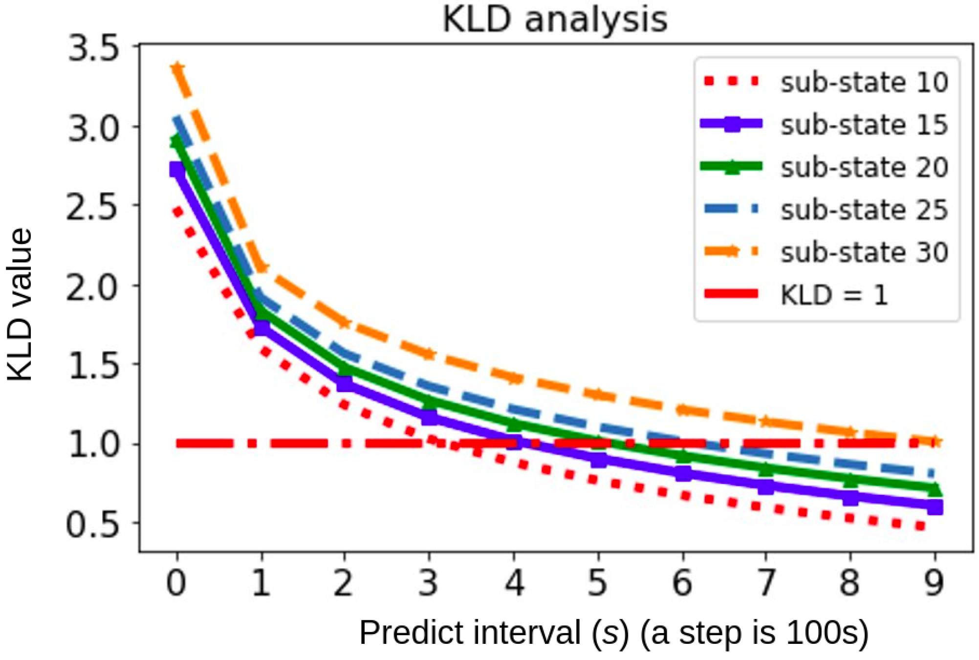
Figure 1. The Thorvald robot in the evaluation environment interacting with the pickers: (a) in a strawberry open field; (b) in a strawberry polytunnel [9].
Agronomy 12 01299 g001
Figure 2. Overview of the anticipatory scheduling strategy in a real strawberry cultivation field.
Agronomy 12 01299 g002
Figure 3. General representation of the topological map and the logical template of a farm field using the DES framework in [4].
Agronomy 12 01299 g003
Figure 4. An example of demo manual picking operation in apple orchard: (a) Picker is picking; (b) Pickers are moving back and forth for loading/unloading trays; (c) Local storage.
Agronomy 12 01299 g004
Figure 5. An example of demo robot-assisted picking operation in apple orchard: (a) Picker is picking; (b) CAR system calling robot; (c) Picker is waiting for robot; (d) Unloading full tray on robot; (e) Local storage.
Agronomy 12 01299 g005
Figure 6. Categorizing the picker’s states: (a) discrete states of picker in robot-assisted picking operation; (b) an example graph showing time duration of each states in a picking operation.
Agronomy 12 01299 g006
Figure 7. Proposed prediction framework: tray_full_node and tray_full_time are the spatio-temporal predictions of “tray-full events”.
Agronomy 12 01299 g007
Figure 8. State transition model used in the proposed spatio-temporal prediction framework.
Agronomy 12 01299 g008
Figure 9. Processes of the prediction framework: from a real-world picking process to the event prediction.
Agronomy 12 01299 g009
Figure 10. KLD analysis for changes in the number of sub-states.
Agronomy 12 01299 g010
Table 1. Changes in the KLD value versus the number of sub-states.
Number of Sub-States1015202530
KLD Value0.460.600.710.921.006
Table 2. List of Acronyms and Abbreviations used in the text with their definition.
AcronymDefinitionDescription
TFTTray Full TimeTime taken to fill a tray, denoted by tray_full_time.
PTEPrediction Time ErrorDifference between actual and predicted t r a y _ f u l l _ t i m e (TFT), denoted by prediction_time_error.
TTTTransportation Time per TrayTravel time taken by picker to unload a full fruit tray to the local storage, denote by transportation_time.
ANCTAverage Nodes Covered per “tray-full event”Nodes distance on an average a picker covers for filling up a tray.
NTTNode Transition TimeTime taken by a picker while picking, to move from one node to its subsequent node.
ATTAverage “tray-full event” TimeFor overall process, an average time taken by a picker to fill a tray.
APCTAverage Process Completion TimeFor overall process, an average time taken to pick a complete farm.
STTSave on Transportation TimeBased on the usage of the prediction model, a reduction in transportation time.
FoOFrequency of OccurrenceLikeliness of an event to occur.
PAEPercentage Average ErrorFor overall process, the absolute difference between actual and predicted values in percent.
Table 3. Analysis of the “tray-full event” for a picker (Id 00).
StartPredictionActualPTE per Tray
EndEnd EndEnd prediction_time_error
ray No.row_IDnode_IDTime (s)Directionrow_IDnode_IDTime (s)Directionrow_IDnode_IDTime (s)DirectionTime (s)
100001.9F00162096.7F00162114.9F18.9
200162393.6F02084630.3F02074475.5F−154.5
302074664.7F02236764.5F02226641.3F−123.2
402226978.1F02118949.0R02118935.6R−13.4
502119163.8R040411,138.5F040411,150.2F11.7
6040411,311.9F041913,281.5F042013,399.4F117.9
7042013,718.8F041315,680.1R041315,686.2R6.1
Table 4. Class categorization of “tray-full event” Predictions based on PTE values.
ClassPred.Act.PTEWho’sEmpiricalFoO
NodeNodeper Tray (s)Waiting% STT (Approx.)
1samesame 0 < PTE ⋘ TTTRobot100High
2behindahead 0 < PTE ≤ TTTRobot ( 80 , 100 )High
3aheadbehind−2TTT ⋘−PTE <−TTTPickerNot ApplicableMedium
4samesame−TTT ⋘ PTE < 0 Picker ( 85 , 100 )Low
Table 5. Overall Picking Operation Analysis Matrix with Values Expressed as mean ± std .
PredictionActualPAE
APCT (s)15,787.85 ± 142.48 15,726.02 ± 56.28 0.38 ± 0.77
ANCT 16.07 ± 0.82 15.78 ± 0.80 1.8 ± 0.10
ATT (s) 2255.26 ± 28.78 2246.57 ± 11.37 0.38 ± 1.09
Publisher’s Note: MDPI stays neutral with regard to jurisdictional claims in published maps and institutional affiliations.

