Article

Greenhouse Thermal Effectiveness to Produce Tomatoes Assessed by a Temperature-Based Index

by
Jorge Flores-Velázquez
1,*,
Fernando Rojano
2,
Cruz Ernesto Aguilar-Rodríguez
3,
Edwin Villagran
4,5 and
Federico Villarreal-Guerrero
6,*
1
Hidrociencias, Colegio de Postgraduados, Campus Montecillos, Carretera México-Texcoco Km. 36.5, Montecillo 56230, Mexico
2
Gus R. Douglass Institute, West Virginia State University, Institute, WV 25112, USA
3
Tecnológico Nacional de México/ITS de Los Reyes, Carretera Los Reyes-Jacona, Col. Libertad, Los Reyes de Salgado 60300, Mexico
4
Department of Biological and Environmental Sciences, Faculty of Natural Sciences and Engineering, Universidad Jorge Tadeo Lozano, Bogotá 110311, Colombia
5
Corporación Colombiana de Investigación Agropecuaria—Agrosavia, Centro de Investigación Tibaitata, Km 14, Vía Mosquera-Bogotá, Mosquera 250040, Colombia
6
Facultad de Zootecnia y Ecología, Universidad Autónoma de Chihuahua, Chihuahua 31453, Mexico
*
Authors to whom correspondence should be addressed.
Agronomy 2022, 12(5), 1158; https://doi.org/10.3390/agronomy12051158
Submission received: 13 March 2022 / Revised: 27 April 2022 / Accepted: 4 May 2022 / Published: 11 May 2022
(This article belongs to the Special Issue Frontier Studies in Agricultural Greenhouse Equipment and Systems)

Abstract

:
This study proposed an indicator to calculate the regional thermal potential from the local temperature. A probabilistic function curve generalized as a complementary error function (erfc) was used to assume the temperature curve follows the normal distribution and considered only the portion of the curve where the appropriate temperatures for the crop are located (wi). The Greenhouse Thermal Effectiveness (GTE) index was calculated using (a) the data of measured temperature (outside) and simulated values from inside of the greenhouse, and (b) the normal temperature data from five meteorological stations. Estimations of GTE using average daily temperature (°C) throughout the year indicate that, with an annual mean temperature of around 14 °C, the GTE is 2798 degree units and inside the greenhouse its value goes up to 5800. May is when the highest temperatures occur and when the highest amount of GTE units can be accumulated. The range of temperatures in the analyzed stations were from 13 to 21 °C and the GTE calculated per year was from 2000 to 7000. The perspective will be to calculate if this energy will be enough to grow tomatoes (or other crops) without extra energy for heating or cooling. If more energy may be needed, estimating how much would be the next step.

1. Introduction

In the coming years, several changes affecting the agriculture sector are expected. Besides the increase in temperature due to climate change, the cost of energy is also expected to increase. Crop production in greenhouses is a strong sink of natural resources. Any change in the climate system implies a modification of the environment that would change the precipitation patterns and the distribution of water. Changes in water distribution and temperature increments will affect the distribution of ecosystems and farming zones [1,2]. Energy has become a currency of change; it has been considered that energy in residential and commercial buildings consumes approximately 40% of the total and represents 36% of the community CO2 emissions [2]. In the agricultural sector, resources are increasingly limited. This has brought unified techniques to achieve the highest yields to feed the growing population with the minimum of resources, mainly water and energy [3].
The evolution of technology applied to crop production aims to satisfy the increasing demand for food by the population, which implies an increase in agricultural activities. The use of energy balance models together with CFD (Computational Fluid Dynamics) has allowed estimating the heating needed to maintain an ideal temperature during the night and grow tomatoes throughout the year. It has also allowed estimating the production costs and the efficiency of the heaters. For instance, Aguilar et al. [4] reported that to maintain a temperature of 12 °C inside the greenhouse in Texcoco, Mexico, during the days with temperatures below the desirable minimum (206 days), 32,228. 76 kWh with a cost of $20,626.40 Mexican pesos (MXN) were needed. Accordingly, Flores-Velázquez et al. [5] estimated the cost of operating a forced cooling system when the temperature exceeds 30 °C inside the greenhouse. Results showed lower costs of forced ventilation for the State of Mexico than for San Luis Potosí, except for the Bejucos station, where costs can go higher than $600.00 MXN.
Some efforts have been made to estimate the heat consumption in semi-closed buildings. Life Cycle Analysis, a recent tool used in this kind of assessment by Decano-Valentin et al. [6], found that the energy used for climate control contributes to 86–96% of the gasses emitted, depending on the type, quantity, and energy source [7,8]. In addition, they used Building Energy Simulation (BES) tools to predict air temperature when using cooling or heating. If the source of energy was electrical, the maximum consumption was between 62.6 kW for cooling and 69.3 KW for heating. Under the climate conditions of South Korea, the average consumption of energy was 811,201 MJ (3,075,520 kW) per year. In experimental greenhouses, Lee et al. [9] reported 68.21% less energy cost using an effluent thermic-heat pump instead of kerosene. At nighttime, crops absorbed 29.54 W m−2 as latent heat and emitted 9.49 W m−2 as thermal energy. In the same study, they quantified cooling loads of 257,482 MJ and heating loads of 813,410 MJ, with a total greenhouse load of 1,070,892 MJ, representing 2934 MJ day−1. In 2022, Reza [10] assessed the energy consumption in two greenhouses covered with two different materials for cucumber production. They built an indicator to describe the energetic intensiveness and found values of 80.26 and 77.07 MJ MXN−1 in each type of greenhouse.
Disruptive techniques have succeeded in increasing production; however, this fact has affected the environment negatively at different scales. Agricultural production efficiency stems from the quest to meet demands with the minimum of natural resources (i.e., soil, water, and energy) and from those agricultural areas where costs can be reduced. Knowing about the renewable energies, which are helpful in a greenhouse, arises as one more factor of resource management for the efficient production of crops [11].
Currently, the climatic needs of tomatoes are known [12] and these may be provided to the greenhouse either passively or through auxiliary systems. To our knowledge, indicators regarding the thermal effectiveness of greenhouses in Mexico have not been reported. In several Mexican regions, the operation of the greenhouse continues being empirical. However, the evaluation of the main greenhouse climatic parameters (i.e., temperature, radiation, and CO2) is needed to know if such parameters are adequate [13]. Temperature is one of the climatic variables that can be effectively measured and modeled; thus, it is possible to generate a-priori information to infer about the dynamics of the climate inside and outside a greenhouse, which is considered useful for planning. To know which of the climate variables (i.e., radiation, temperature, and relative humidity) is really contributing to the development of the crop on a daily, monthly, and cycle basis, is key for appropriate decision making. The use of a mathematical function to build and calculate the Greenhouse Thermal Effectiveness (GTE) and the Greenhouse Thermal Potential (GTP) allows us to infer about the local or regional thermal potential by visualizing the number of days the temperature will be within a suitable range for cultivation to prevent reductions of yield [12]. It is important to address the efficient use of the climatic resources to eliminate or reduce the use of auxiliary systems for climate control, such as heating and cooling.
Several tools and some indicators have been studied to infer about the climate dynamics [14]. Life cycle analysis is one way to analyze the energy consumption in several process, mainly during the construction and during the use of energetic sources. In accordance with the above, there are several studies that determined heating activities are the ones that produce the highest energy consumption, with costs that even exceed 50% of total production costs [15]. In addition, the consumption of gas and electric energy for heating is one of the energy sources generating the greatest negative environmental impact in the production systems of the main horticultural species under greenhouse conditions [16]. For example, Samaranayake et al. [17] reported that the energy consumption in a high-tech greenhouse with a Capsicum crop located in Australia for an 8-month growing cycle was 14.6 kWh and 2.2 kWh for 1 °C heating and cooling, respectively.
The current agricultural activity has also generated increments in production and, consequently, environmental negative impacts. To increase production, it is necessary to do research and satisfy increased demands with the optimization of agricultural land and water [18]. In a study of a crop’s productive potential, two fundamental processes are necessary: the definition of the crop’s agroecological requirements and their comparison with the region’s environmental conditions where it is intended to be produced [19]. Experimental and numerical models have been implemented to measure climatic variables and crop production [2]. They proposed indexes such as cumulative solar radiation (CSR) or Cumulative Heat Unit (CHU) and found a robust relationship between the climate and the agronomic characteristics.
There exists a relationship between climatologic variables, such as temperature [20,21,22,23], CO2, humidity, and vapor pressure deficit with crop production [24]. Temperature is the primary variable related to the development of plants. Conceptually, the generation of indicators or indexes is based mainly on thermal requirements by crops to complete each one of their phenological stages or the whole crop cycle [25,26]. Based on the physiological conditions of crops, Marcelis et al. [26] studied the need to apply biological models in order to save energy to get a low-cost crop production. Almanza-Merchan et al. [27] used the absolute growth rate (AGR), which indicates the change in size per unit of time, and the relative growth rate (RGR) to define the variation of rate of size per initial size unit (dry mass accumulation), which was valuable for determining the growth per time and finding similar results to Ardila et al. [28].
Several indicators have been established to characterize the development of crops and the operation of greenhouses related to climatic variables [29]. In some cases, the objective is to define the beginning or end of stages, which are necessary to complete the cycle. For example, the degree days of growth (°D) indicate the development of living organisms, which depend linearly on temperature (°C). Similar indicators have been created to quantify the heating and cooling requirements in specific regions [3,30], which is needed to calculate the energy consumption.
Regarding water use efficiency, this parameter has been used for programming irrigation to potatoes [31]. The use of this concept has recently jumped to crops in greenhouse systems, specifically tomatoes [28,32] and peppers [33], to calculate Heating Degree Days (HDD) as an indicator of heat requirements by the crops. These studies indicate that tomatoes require 2400 HDD to complete their development cycle and estimates the heating needs for greenhouse operation as a function of temperature [34,35].
With the advances in meteorology and cultivation techniques, traditional indexes to measure crop requirements by phenological stages also need to get improved. For instance, the regional thermal potential indicates how much heat is produced (received) in a specific crop productive region and what kind of crops have the most significant probability of getting a complete life cycle in a short time [36]. This is a space–time indicator of heat quantity distribution, not only under open field but also under greenhouse conditions. Therefore, climate data becomes key in the decision-making related to agriculture and the study of climatic variables, and their distribution are essential for farming zones [19,37]. Similarly, one way to study the effect of climatic variables on crops under controlled environments is by generating models with numerical solutions.
For instance, success in tomato production depends on the accomplishment of the temperature requirement [13]. A study by Jones et al. [37] found that the optimal average temperature is 23 °C, similar to the findings of Atherton and Rudich [38]. During one single day. Other research [39,40,41,42] affirmed that for the development of a tomato crop, the effect of temperature integrated daily is better than daily temperature oscillation. In that study, temperatures ranged between 22 to 26 °C during the day and 13 to 16 °C during the night [43].
Some countries have been focused on reducing the fossil energy use in agriculture, especially under protected agriculture. Some tropical regions are better than cool regions for crop productions under greenhouses. To know the potential of a specific region for production, characterization should be carried out. The determination of productive potential for a specific region has been of particular interest for outdoor and seasonal crops [19,44]. In the studies of productive potential, climatic, orographic, and soil factors have been mainly considered. In addition, the potential production of several crops has been analyzed in studies with regional impact [19,36,45]. Therefore, thermal integration can be applied to greenhouses as an efficiency index, even though the temperature in the greenhouse depends on the radiation quantity in each specific region [19,46]. These studies can be adapted to protected agriculture, since a partial or total control of environmental variables affects crop development. If the system is fully enclosed and automated (high-tech greenhouses), external environmental conditions have less impact, while the opposite is true for medium and low-tech greenhouses. Therefore, this study is focused mainly on medium and low-tech installations, where it is possible to take advantage of the regional climatic factors to increase production per area [19,47].
The objective of this work was to propose an indicator to calculate the regional thermal potential from the local temperature. A probabilistic function curve (erfc) was used to assume the temperature curve follows a normal probability distribution function and considered only the portion of the curve where the temperature is appropriate for the crops. The temperature was set as the main climatic factor to obtain an optimal microclimate for the crops. An indicator was used to calculate the thermal potential in central Mexico. The climate index shows the region’s suitability to achieve high yields croping under low-tech greenhouses.

2. Materials and Methods

2.1. Theory of the Thermal Index in Crops

The average temperature in a day through the years presents a normal probability distribution [20] with a mean (Tmed) and amplitude as standard deviation. The mean positions the curve on the x-axis while the temperature t, and the deviation determines its position as the curve opens on the x-axis [21]. The frequency amplitude depends on the geographic location defined by the mean (T). The mean can determine and move the curve to the left or right based on the geographic location (To) [22].
The concept of heating days refers to the amount of energy stored per day and is related to the number of sunny and shady hours. The probability curve for temperature resembles the probability curve for HDD. Changes in the location and scale length (t) in the temperature frequency distribution also cause changes in the frequency curve of the HDD curve [46].
Many authors have computed the HDD to analyze the effect on the growth of tomatoes [45], to estimate heating and cooling days [30], heating requirements for crops under open field [46], energy requirements for a greenhouse [48], and several other analyses for greenhouses [30,33,49]. However, these calculations are based on statistical values. The complementary error function may be used assuming the same behavior of the statistical probability curve of temperature [31] and HDD. The erfc has been used as a predictive model and as a probabilistic function [50] calculating the area under the curve as cumulative heat by the crops and management of other activities such as irrigation programming or heating/cooling design of mechanical systems [45,51,52,53,54].
The proposal of a thermal index for greenhouse characterization is based on the fact that all crops need some temperature level to complete their physiological cycle [25,47,48]. Temperature oscillation depends on local conditions, specific latitude, and altitude (T med and standard deviations). The erfc curve is always the same for one kind of crop; for instance, for tomato, the optimal temperature (Te) and the amplitude (A) are the same regardless of the geographic localization. If the optimum temperature remains constant during the day, the effectiveness of the greenhouse will be 100%. If the temperature is lower or higher than optimum, just a portion of this temperature is approaching; as a consequence, the efficiency of the greenhouse will be lower than 100% [19].
Based on previous analyses of the index [30,51,52], Equation (1) was used to calculate the proportion of temperature used by the crop. The estimation of temperature effectiveness is done by using an equation that defines a proportion function (wi) as shown in Equation (1) [19]:
w i = e r f c T i T e 2 A 2 T i
where A is the amplitude of the variable or standard deviations of the probabilistic curve (σ), Ti is the observed temperature value (°C), and Te is the optimal value of the variable (T med in the probabilistic curve). The values of Te and A are defined according to the optimum values reported by the literature for the crops to be analyzed.
The climatic variable recorded in the greenhouse may approach the optimal average, considering the maximum effectiveness when it tends to the unit. For example, the tomato (Solanum lycopersicum L.) has an optimal average daily mean temperature (Te) of 23 °C and an amplitude A = 12 °C [53,54,55,56].

2.2. Error Function Complementary (erfc) Conceptual Applications

The average temperature in a day through the years presents a normal probability distribution [18] with a mean (Tmed) and amplitude as standard deviation. The mean places the curve on the x-axis while the temperature t and the deviation determines its position as the curve opens on the x-axis [22,23]. The frequency amplitude depends on the geographic location defined by the mean (T). The mean can determine and move the curve to the left or right based on geographic location (To) [19].
The complementary error function plays a role in asymptotic problems of integrals when a saddle point and a pole are close together or even coalesce. It also occurs typically when a saddle point is near a point on the integration interval [19,49].
The erfc can be written as Equation (2)
e r f c z = 2 π   z e t 2 d t
It is a defined integral tending to infinite, which can be rewritten as Equation (3) [57]
w z = 1 π i     e t 2 t z d t
Several ways to generalize this equation are possible as a function of the use. The erfc (x) function represents the complementary error function. The function is a rational approximation of the erfc (x) function, for z   0 , represented by [55] is given by Equation (4):
e r f c x = 1 + k = 1 4 a k   z k 4
where z is a wi and k are the values of 1–4. A rational approximation was fixed with Taylor series, and the results are k1 = 0.278393, k2 = 0.230389, k3 = 0.000972, and k4 = 0.078108 [56,57].
This function was used in this work to adapt the curve of temperature with a curve representing an approximation of effectiveness of greenhouses based in a part of these temperatures, which represent the inner range used for the crop. The quantity of the Greenhouse Thermal Effectiveness (GTE) for a daily temperature (Ti) can be estimated with the Equation (5):
GTE = ω i T i
If the daily ambient temperature Tj is close to the optimal value Te, the wj value is close to one, and consecutively, the Greenhouse Thermal Effectiveness (GTE (°)) is close to Te [19].
Accumulated GTE quantitatively defined the effectiveness of a greenhouse in maintaining potential conditions for crop development. The cumulative values or Greenhouse Thermal Potential (GTP) of GTE (°) were estimated according to Equation (6): [19]
GTE = i = 1 N ω i T i = i = 1 N GTP
where N is the period under study. The period of study can be established per day, with a sensor inside or outside the greenhouse, and data were collected along the day (real approximation) or with average daily temperature (average approximation).

2.3. Temperature Database Used to Estimate GTE

As shown in Equations (1) and (6), the temperature is the primary variable to estimate the thermal indicator. Therefore, several options can be selected to define the type of data to work, considering frequency, period, etc. If there is a measured temperature, it is possible to get the best approximation of the indicator in real-time. Other options are available to using daily average temperature or monthly average temperature.
In this case, the thermal proposal indicator was estimated using daily and monthly average temperatures from two temperature sources (i) Normal database of climatic stations close to the zone analyzed and (ii) measured temperature outside the greenhouse. Then, both options can be used as a boundary condition based on outside temperature and wind velocity to obtain the temperature (simulated) inside the greenhouse; after simulation, the temperature was used to calculate the greenhouse GTE (Figure 1).
The results of the simulations were obtained considering as boundary condition the monthly mean temperature, used to predict the internal climatic conditions of the greenhouse at the level of the growing area. The greenhouse characteristics, sensors of temperature, and experimental setup is described in [Appendix A]. In this work, the same boundary conditions were used to calculate GTE outside of the greenhouse. After that, a temperature simulated at 0.9 m of height from the ground level was used to calculate an average in each greenhouse span. In this study, greenhouse temperatures were simulated for each month and then GTE and GTP were calculated to know the climatic potential to produce tomato along the year.

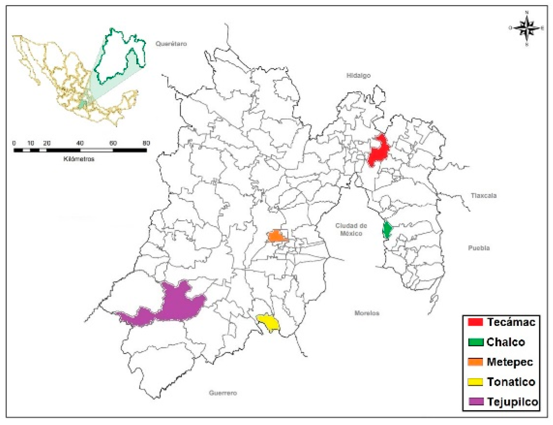
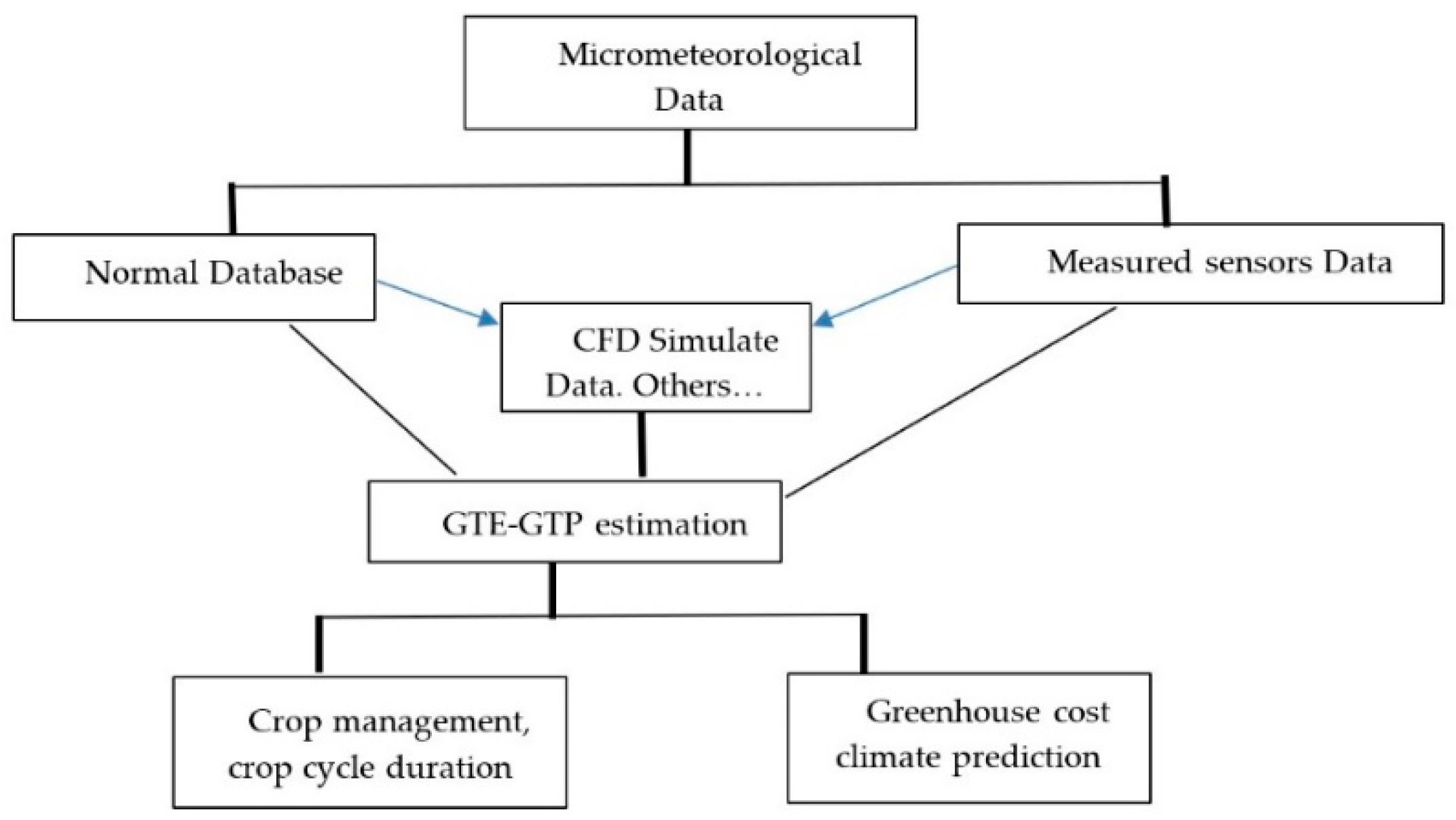
2.4. Estimation of GTE and Extrapolation to the State of Mexico (Central Mexico)

In addition to knowing the climatic potential by using the proposed indicator, this study also analyzed the productive potential for a region. For that, GTE was estimated with data from five weather stations located in Central Mexico (Figure 2), considering the average daily temperature Ti (364 days) during more than 24 years [19].
Thermal efficiency was evaluated considering ranges from 20 to 100%, during spring-summer and autumn–winter according to SAGARPA-SIAP [58]. The Mexican agricultural production is divided into two periods: spring–summer and autumn–winter. The former runs from March to September while the latter runs from October to February.

3. Results

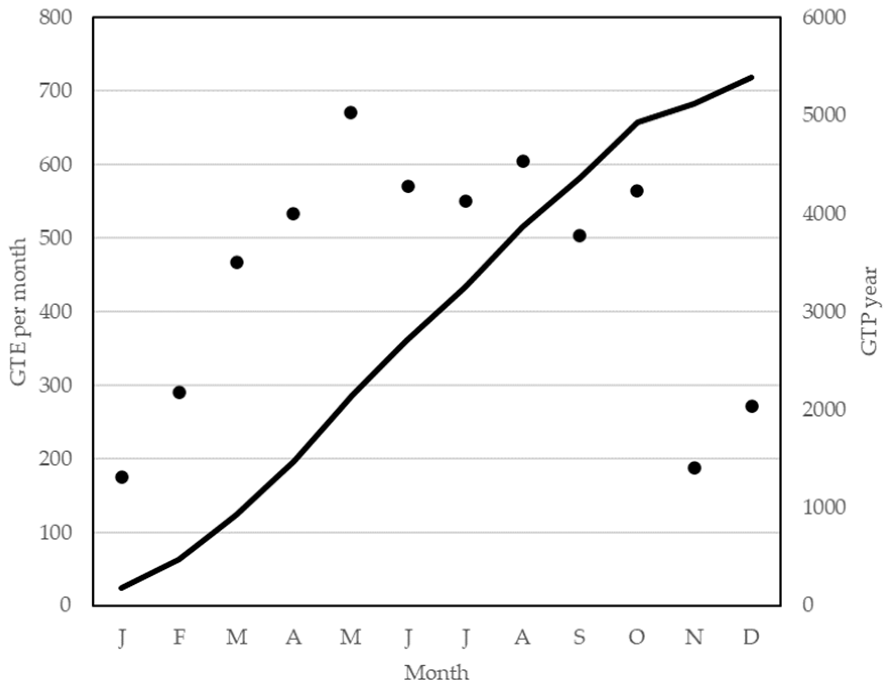
3.1. Greenhouse Thermal Effectiveness Estimation and Comparative Results

The first approximation for the outside temperature was carried out in a greenhouse in Central Mexico (Chapingo, Mexico) to standardize the temperature data, regardless of the source (measured, database, or simulated). Then, GTE was estimated using the average monthly temperature. Two sources of temperature data were used: a typical database with data from the Chapingo climatic station, and measured data to improve the accuracy of GTE (Figure 3).

3.2. Greenhouse Thermal Effectiveness by Using the Database of Temperature

The average daily temperature (°C) from five meteorological stations was used to estimate the GTE. Figure 4 shows the values of the Greenhouse Thermal Efficiency (GTE) and the accumulated value in one year (GTP) for central Mexico. Under these average temperature conditions throughout the year, ranges of degree units from 2000 to more than 7000 were obtained, May being the month with the highest temperature, and therefore, more energy can be accumulated in the greenhouse (Figure 5).
The thermal efficiency of the greenhouse to generate an optimum temperature range for the tomato crop is shown in Figure 5. Outside the greenhouse, the maximum amount of GTP per year (i.e., Chalco) was around 2700. Inside the greenhouse, the GTP increased to 5800. Therefore, the GTE is an index that could be used to plan the crop season (Figure 5). In addition, this index can help determine crop planting dates to plan the harvest dates with the best window to the market.
A practical way to estimate GTE is using the average temperature, which is a variable measured in all of the meteorological stations. Table 1 shows the variation of average temperatures (minimum, maximum, and mean). The mean temperature was used to estimate the potential of these regions to produce the tomatoes per cycle (Spring–Summer and Autumn–Winter).
The comparison of the five stations indicates that Tonatico and Tejupilco had the highest thermal efficiencies throughout the year because they were in areas with average temperatures around 20.0 °C (the warmest in central Mexico). The Tecámac station was located in a zone with moderate average temperatures, so the thermal efficiency dropped to 40%, maintaining the highest efficiency in spring–summer. The station with the lowest efficiencies was Metepec since it is located in the mountainous area near the Toluca volcano, where average daily temperatures are low (13.2 °C).
The potential can be also estimated as a function of the range of days within the minimum and maximum temperatures. The GTE can be divided into five ranges of effectiveness to compute how many days the environment generates conditions to grow the crop in the greenhouse. Table 2 shows the result of these estimations in the two typical crop cycles. Spring–Summer with 210 days and Autumn–Winter with 140 days per cycle. The difference in days of the cycle is due to the temperature that slowly rises, the cost of operation in the greenhouse, and the cost of the produce.
The degree units accumulated depends on the geographic location. If it is analyzed for several agroclimatic stations and spread on a spatial map, it is possible to illustrate the distribution of GTE [19]. The Kriging Interpolation method was used to determine the GTE spatial distribution. Figure 6 shows the cumulative GTP for the state of Mexico (Central Mexico) using data from the meteorological stations and estimating minimum, maximum, and average temperatures in the year.

4. Discussion

Unlike some studies [30,47] that were only used to estimate the thermal efficiency of greenhouses with simulated and measured data, this work shows greater accuracy by standardizing the temperature data (measured, database, or simulated), making it more reliable at the time of its use (Figure 3). Figure 4 shows that the highest thermal efficiency in central Mexico is above 60% (i.e., Chalco) and occurs during spring–summer. Meanwhile, during autumn–winter, days have an average thermal efficiency between 20 and 40% in the same station. Therefore, the spring–summer is the more suitable period while it is not advisable to cultivate tomatoes in the autumn–winter period.
For the five stations analyzed (Table 1), the thermal efficiencies of spring–summer was above 40%. During mid-March, the thermal efficiency increased in the cold stations above 60% until mid-August. In the case of the hot stations, thermal efficiency decreased in May due to the high temperatures recorded in that month. Higher temperatures also decreased thermal efficiency since they were far from the optimal temperature for tomatoes. Even though the weight function decreased, it maintained higher values than the optimal set point.
Temperature is a crucial climatic factor to know about for the potential of agriculture under open field conditions, not only to detect the beginning of the growing season but also in the operation and climate control of greenhouse systems. Figure 4 shows that in Tonatico and Tejupilco, there was a better distribution of the thermal efficiency throughout the year for the tomato crop. For Chalco, Tecamac, and Metepec, the highest thermal efficiency recorded was during spring–summer; however, it is not possible to complete a tomato cycle during the winter, so it is recommended to grow a crop that is adapted to the conditions of the area.
The spatial distribution of Figure 6 represents a tool for decision-making to define the best climatic zones to build greenhouses [33]. Based on the zone, it can be estimated if auxiliary equipment has to be used seasonally or continuously, which will directly affect production costs [43]. In the north–central region of the state of Mexico, the prevailing GTE was low (<2000), which indicates the climate is not appropriate to complete the cycle of tomatoes. However, other crops demand temperatures in the ranges found for that region, and with shorter phenological cycles, may be produced in these regions [19].

5. Conclusions

The indexes of GTE and GTP were used to characterize potential areas to produce tomato under greenhouse conditions based on simulated and measured temperatures. The adequation of the complementary error function (erfc) as a representation of temperature distribution was applied as an index considering the optimal requirement of temperature for tomatoes. This research allowed analysis of the GTE when considering five meteorological stations located in central Mexico. The proposed index can estimate the thermal efficiency of a low-tech greenhouse in any region. In addition, this index could help to define regions with suitable climatic conditions for any crop, either produced under open fields or under greenhouse conditions.
The indicator can also be implemented for climate control since it is an easy numerical implementation to estimate the effectiveness of a climatic variable to provide optimum conditions for a crop. The lower the GTE, the greater the need for heating or cooling.

Author Contributions

J.F.-V. (Conceptualization and methodology, formal analysis); F.R. (investigation, writing—original draft preparation and validation); C.E.A.-R. (software, data curation and formal analysis); E.V. (software, data curation, review, and editing); F.V.-G. (methodology, investigation, and writing—review and editing). All authors have read and agreed to the published version of the manuscript.

Funding

This research received no external funding.

Data Availability Statement

Did not report any data.

Conflicts of Interest

The authors declare no conflict of interest.

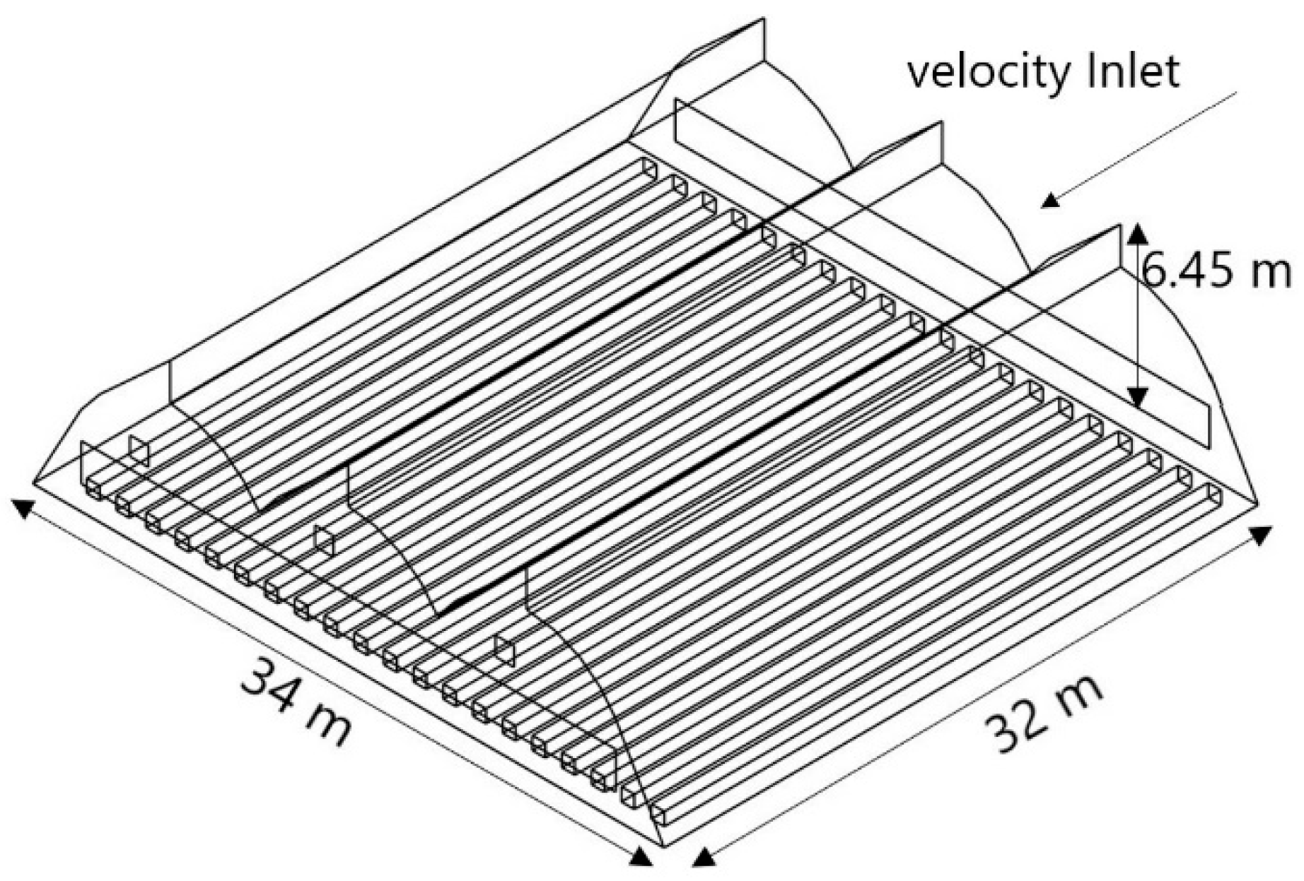
Appendix A. CFD Model

The computational model was built in ANSYS® Fluent®. The geometry was elaborated in ANSYS® Workbench using Design Modeler. A sensitivity analysis of the greenhouse mesh was performed to obtain a reliable model. For that, measurements of temperature at 100 points located elevated 2 m from the ground level were made longitudinally inside the greenhouse. The analysis was performed considering four scenarios; the number of mesh elements varied among the scenarios. There were no differences between the simulated temperature resulting from a mesh of 400,000 elements and meshes with a higher number of elements. The model with a mesh of 416,113 structured elements with an orthogonal quality of 0.96776 and a skewness of 2.0639 × 10⁻² was used. Table A1 shows the setting and the boundary conditions applied to such a model and Figure A1 depicts the general dimensions of the experimental greenhouse.
Table A1. Setting and boundary conditions of the CFD model.
Boundary ConditionsMethod
SolverPressure-based
StateSteady
Viscosity functionk-ε Standard
Energy equationActivated
EntryVelocity inlet
OutputPressure outlet
Air temperatureConstant (22.55 °C)
Wind speedConstant (2.41 m s−1)
Porous jumpPermeability face
Thin porous media
Drag coefficient
Heat sourceBoussinesq’s hypothesis
Soil thermal conditionConstant (200 W m−2)
To assess the reliability of the CFD model, the root mean square error (RMSE) was used as a goodness-of-fit test. The RMSE was computed with the deviations found between the simulated values of the variables and the values retrieved from the greenhouse sensors.
Figure A1. Dimensions of the experimental greenhouse.
Agronomy 12 01158 g0a1
The period of from 12:30 to 13:00 was considered in the evaluation to obtain a reliable model. The measured and simulated temperature data is shown in Table A2. The computed RMSE was 1.93 °C, equivalent to 7.31% of the temperature mean estimated with measured values inside the greenhouse. These results are consistent with previous studies employing the same approach [59,60]. With that, we assumed the reliability of the prediction model was good to be used in our study.
Table A2. Measured and simulated temperature data (°C).
SensorsExperimentalSimulated
125.524.9
225.725.5
328.525.1
426.323.9
525.726.6

References

  1. Moreno, R.A.; Aguilar, D.J.; Luévano, G.A. Características de la agricultura protegida y su entorno en México. Rev. Mex. Agroneg. 2011, 15, 763–774. [Google Scholar]
  2. Doan, C.C.; Tanaka, M. Relationships between Tomato Cluster Growth Indices and Cumulative Environmental Factors during Greenhouse Cultivation. Sci. Hortic. 2022, 295, 110803. [Google Scholar] [CrossRef]
  3. Park, S.; Shim, J.; Song, D. Issues in calculation of balance-point temperatures for heating degree-days for the development of building-energy policy. Renew. Sustain. Energy Rev. 2021, 135, 110211. [Google Scholar] [CrossRef]
  4. Aguilar-Rodriguez, C.E.; Flores-Velazquez, J.; Ojeda-Bustamante, W.; Rojano, F.; Iñiguez-Covarrubias, M. Valuation of the Energy Performance of a Greenhouse with an Electric Heater Using Numerical Simulations. Processes 2020, 8, 600. [Google Scholar] [CrossRef]
  5. Flores-Velázquez, J.; Vega-García, M. Regional management of the environment in a zenith greenhouse with computational fluid dynamics (CFD). Ing. Agríc. Biosist. 2019, 11, 3–20. [Google Scholar] [CrossRef]
  6. Decano-Valentin, C.; Lee, I.B.; Yeo, U.H.; Lee, S.Y.; Kim, J.G.; Park, S.J.; Choi, Y.B.; Cho, J.H.; Jeong, H.H. Integrated Building Energy Simulation–Life Cycle Assessment (BES–LCA) Approach for Environmental Assessment of Agricultural Building: A Review and Application to Greenhouse Heating Systems. Agronomy 2021, 11, 1230. [Google Scholar] [CrossRef]
  7. Villagran, E.; Bojacá, C.; Akrami, M. Contribution to the Sustainability of Agricultural Production in Greenhouses Built on Slope Soils: A Numerical Study of the Microclimatic Behavior of a Typical Colombian Structure. Sustainability 2021, 13, 4748. [Google Scholar] [CrossRef]
  8. Rabbi, B.; Chen, Z.H.; Sethuvenkatraman, S. Protected Cropping in Warm Climates: A Review of Humidity Control and Cooling Methods. Energies 2019, 12, 2737. [Google Scholar] [CrossRef] [Green Version]
  9. Lee, S.Y.; Lee, I.B.; Lee, S.N.; Yeo, U.H.; Kim, J.G.; Kim, R.W.; Decano-Valentin, C. Dynamic Energy Exchange Modelling for a Plastic-Covered Multi-Span Greenhouse Utilizing a Thermal Effluent from Power Plant. Agronomy 2021, 11, 1461. [Google Scholar] [CrossRef]
  10. Reza, H.; Morteza, T.; Rostam, F.; Mehrdad, H.; Anthony, H. Energy-economic-environmental cycle evaluation comparing two polyethylene and polycarbonate plastic greenhouses in cucumber production (from production to packaging and distribution). Sci. Total Environ. 2022, 828, 154232. [Google Scholar]
  11. Latin American and Caribbean Demographic Centre CELADE. World Population and Latin America and the Caribbean Population: Changes and New (Im) Balances; Astrolabio, Universidad Nacional de Cordoba. Argentina No. 8; Universidad Nacional de Córdoba: Córdoba, Argentina, 2012. [Google Scholar]
  12. Nurdan, Y.; Levent, B. Evaluation of a hybrid system for a nearly zero energy greenhouse. Energy Convers. Manag. 2017, 148, 1278–1290. [Google Scholar]
  13. Mukesh, K.; Didier, H.; Stéphane, G. Survey and evaluation of solar technologies for agricultural greenhouse application. Sol. Energy 2022, 232, 18–34. [Google Scholar]
  14. Farzin, G.; Niko, H.; Stefanie, H.; Ramin, R. A novel integrated framework to evaluate greenhouse energy demand and crop yield production. Renew. Sustain. Energy Rev. 2018, 96, 487–501. [Google Scholar]
  15. Shen, Y.; Wei, R.; Xu, L. Energy Consumption Prediction of a Greenhouse and Optimization of Daily Average Temperature. Energies 2018, 11, 65. [Google Scholar] [CrossRef] [Green Version]
  16. Naderi, S.A.; Dehkordi, A.L.; Taki, M. Energy and Environmental Evaluation of Greenhouse Bell Pepper Production with Life Cycle Assessment Approach. Environ. Sustain. Indic. 2019, 3, 100011. [Google Scholar] [CrossRef]
  17. Samaranayake, P.; Liang, W.; Chen, Z.-H.; Tissue, D.; Lan, Y.-C. Sustainable Protected Cropping: A Case Study of Seasonal Impacts on Greenhouse Energy Consumption during Capsicum Production. Energies 2020, 13, 4468. [Google Scholar] [CrossRef]
  18. Al-Kodmany, K. The Vertical Farm: A Review of Developments and Implications for the Vertical City. Buildings 2018, 8, 24. [Google Scholar] [CrossRef] [Green Version]
  19. Flores-Velazquez, J.; Aguilar, R.C.E.; Ojeda, W.; Rojano, F. CFD index for temperature greenhouse characterization. In Proceedings of the 2018 ASABE Annual International Meeting, Detroit, MI, USA, 29 July–1 August 2018. [Google Scholar]
  20. Armendáriz-Erives, S. Desafíos y riesgos agrícolas ante el calentamiento global. In Oportunidades y Retos de la Ingeniería Agrícola Ante la Globalización y el Cambio Climático; UACH-URUZA: Durango, Mexico, 2007; pp. 73–79. [Google Scholar]
  21. Thom, H.C.S. Seasonal Degree-day statistic for the United States. Mon. Weather Rev. 1952, 80, 143–149. [Google Scholar] [CrossRef] [Green Version]
  22. Thom, H.C.S. The rational relationship between heating degree-day and Temperature. Mon. Weather Rev. 1954, 82, 1–6. [Google Scholar] [CrossRef] [Green Version]
  23. Thom, H.C.S. Some Methods of Climatological Analysis; WMO Technical Note Number 81; Secretariat of the World Meteorological Organization: Geneva, Switzerland, 1956; p. 53. [Google Scholar]
  24. Shamshiri, R.; Jones, J.W.; Thorp, K.; Ahmad, D.; Man, H.; Taheri, S. Microclimate evaluation and control in greenhouse cultivation of tomato: A review. Int. Agrophys. 2018, 32, 287–302. [Google Scholar] [CrossRef]
  25. Lin, D.; Wei, R.; Xu, L. An integrated yield prediction model for greenhouse tomato. Agronomy 2019, 9, 873. [Google Scholar] [CrossRef] [Green Version]
  26. Marcelis, L.F.M.; Buwalda, F.; Dieleman, J.A.; Dueck, T.A.; Elings, A.; de Gelder, A.; Hemming, S.; Kempkes, F.L.K.; Li, T.; van Noort, F.; et al. Innovations in crop production: A matter of physiology and technology. Acta Hortic. 2014, 1037, 39–45. [Google Scholar] [CrossRef]
  27. Almanza-Merchán, P.J.; Arévalo, Y.A.; Cely, R.G.E.; Pinzón, E.H.; Serrano, C.P.A. Caracterización del crecimiento del fruto de tomate (Solanum lycopersicum L.) híbrido ‘Ichiban’ cultivado bajo cubierta. Agron. Colomb. 2016, 34, 155–162. [Google Scholar] [CrossRef]
  28. Ardila, G.; Fischer, G.; Balaguera-López, H.E. Caracterización del Crecimiento del Fruto y Producción de Tres Híbridos de Tomate (Solanum lycopersicum L.) en Tiempo Fisiológico Bajo Invernadero. Rev. Colomb. Cienc. Hortíc. 2011, 5, 44–56. [Google Scholar] [CrossRef] [Green Version]
  29. Holmes, C.; Tett, S.; Butler, A. What is the uncertainty in degree-day projections due to different calibration methodologies? J. Clim. 2017, 30, 9059–9075. [Google Scholar] [CrossRef]
  30. Ojeda-Bustamante, W.; Sifuentes-Ibarra, E.; Slack, D.C.; Carrillo, M. Generalization of Irrigation Scheduling Parameters Using the Growing Degree Days Concept: Application to a Potato Crop. Irrig. Drain. 2004, 53, 251–261. [Google Scholar] [CrossRef]
  31. Aguilar-Rodriguez, C.E.; Flores-Velazquez, J.; Rojano-Aguilar, F.; Ojeda-Bustamante, W.; Iñiguez-Covarrubias, M. Crop cycle estimation in greenhouse, based on degree day heat (GDC) simulated in CFD. Tecnol. Cienc. Agua 2020, 11, 27–57. [Google Scholar]
  32. Atilgan, A.; Tezcan, A. Evaluation of Temperature Data Usage the Method of Degree-Hour in Greenhouses: Pepper Plant Case. Sci. Pap. Ser. B Hortic. J. 2017, 61, 287–292. [Google Scholar]
  33. Mourshed, M. Relationship Between Annual Mean Temperature and Degree-Days. Energy Build. 2012, 54, 418–425. [Google Scholar] [CrossRef] [Green Version]
  34. Coskun, C.; Ertürk, M.; Oktay, Z.; Hepbasli, A. A new approach to determine the outdoor temperature distributions for building energy calculations. Energy Convers. Manag. 2014, 78, 165–172. [Google Scholar] [CrossRef]
  35. Djebli, A.; Hanini, S.; Badaoui, O.; Haddad, B.; Benhamou, A. Modeling and comparative analysis of solar drying behavior of potatoes. Renew. Energy 2020, 145, 1494–1506. [Google Scholar] [CrossRef]
  36. Yildiz, I.; Sosaoglu, B. Spatial Distributions of Heating, Cooling, and Industrial Degree-Days in Turkey. Theor. Appl. Climatol. 2007, 90, 249–261. [Google Scholar] [CrossRef] [Green Version]
  37. Jones, J.W.; Kenig, A.; Vallejos, C.E. Reduced state–Variable tomato growth model. ASABE 1999, 42, 255–265. [Google Scholar] [CrossRef]
  38. Atherton, J.G.; Rudich, J. The Tomato Crop; Chapman and Hall: London, UK; New York, NY, USA, 1986; p. 661. [Google Scholar]
  39. Heuvelink, E. Influence of day and night temperature on the growth of young tomato plants. Sci. Hortic. 1989, 38, 11–22. [Google Scholar] [CrossRef]
  40. De Koning, A.N.M. Long term temperature integration of tomato. Growth and development under alternating temperature regimes. Sci. Hortic. 1990, 45, 117–127. [Google Scholar] [CrossRef]
  41. Körner, O.; Challa, H. Design for an improved temperature integration concept in greenhouse cultivation. Comput. Electron. Agric. 2003, 39, 39–59. [Google Scholar] [CrossRef]
  42. Tesi, R. Medios de Protección Para la Hortofloro Fruticultura y el Viverismo; Mundi-Prensa: Madrid, Spain, 2001; p. 288. [Google Scholar]
  43. Anandhi, A. Growing degree days—Ecosystem indicator for changing diurnal temperatures and their impact on corn growth stages in Kansas. Ecol. Indic. 2016, 61, 149–158. [Google Scholar] [CrossRef] [Green Version]
  44. Pathak, T.B.; Stoddard, C.S. Climate change effects on the processing tomato growing season in California using growing degree day model. Model. Earth Syst. Environ. 2018, 4, 765–775. [Google Scholar] [CrossRef]
  45. Grigorieva, E.; Matzarakis, A.; De Freitas, C. Analysis of growing degree-days as climate impact indicator in a region with extreme annual air temperature amplitude. Clim. Res. 2010, 42, 143–154. [Google Scholar] [CrossRef] [Green Version]
  46. Semple, L.; Carriveau, R.; Ting, D. Assessing heating and cooling demands of closed greenhouse systems in a cold climate. Int. J. Energy Res. 2017, 41, 1903–1913. [Google Scholar] [CrossRef]
  47. Soussi, M.; Chaibi, M.T.; Buchholz, M.; Saghrouni, Z. Comprehensive Review on Climate Control and Cooling Systems in Greenhouses under Hot and Arid Conditions. Agronomy 2022, 12, 626. [Google Scholar] [CrossRef]
  48. Kraemer, M.E.; Mullins, C.D.; Nidziela, C.E., Jr. Effect of greenhouse temperature on tomato yield and ripening. Va. J. Sci. 2012, 63, 4–14. [Google Scholar]
  49. Deaño, A.; Temme, N.M. Analytical and numerical aspects of a generalization of the complementary error function. Appl. Math. Comput. 2010, 216, 3680–3693. [Google Scholar] [CrossRef] [Green Version]
  50. Li, S.W.; Li, H.; Han, X.; Ma, Y. Development and validation of a model for whole course aging of nickel added to a wide range of soils using a complementary error function. Geoderma 2019, 348, 54–59. [Google Scholar] [CrossRef]
  51. Faridi, H.; Arabhosseini, A.; Zarei, G.; Okos, M. Degree-Day Index for Estimating the Thermal Requirements of a Greenhouse Equipped with an Air-Earth Heat Exchanger System. J. Agric. Mach. 2021, 11, 83–95. [Google Scholar]
  52. Lebedev, N.N. Special Functions and their Applications. Am. Math. Mon. 1966, 1, 308. [Google Scholar] [CrossRef]
  53. Chevillard, S. The functions erf and erfc computed with arbitrary precision and explicit error bounds. Inf. Comput. 2012, 216, 72–95. [Google Scholar] [CrossRef] [Green Version]
  54. Hannan, J.J. Greenhouses, Advanced Technology for Protected Horticulture; CRC Press: Boca Raton, FL, USA, 1997; 708p. [Google Scholar]
  55. Sato, S.; Peet, M.M.; Thomas, J.F. Physiological factors limit fruit set tomate (Lycopersicon esculentum Mill.) under chronic, mild heat stress. Plant Cell Environ. 2000, 23, 719–726. [Google Scholar] [CrossRef]
  56. Abramowitz, M.; Stegun, I. Handbook of Mathematical Function; Dover: New York, NY, USA, 1972; p. 299. [Google Scholar]
  57. Flores-Velazquez, J.; Ojeda-Bustamante, W.; Salazar, I.; Rojano, A.; López, I. Water Requirements for Greenhouse Tomato. Terra Latinoam. 2007, 25, 127–134. [Google Scholar]
  58. SAGARPA-SIAP. Superficie Agrícola Protegida. 2017. Available online: http://www.sagarpa.gob.mx/quienesomos/datosabiertos/siap/Paginas/superficie_agricola_protegida.aspx (accessed on 10 November 2018).
  59. Silva, R.C.D.; Cordeiro, J.J.; Pandorfi, H.; Vigoderis, R.B.; Guiselini, C. Simulation of ventilation systems in a protected environment using computational fluid dynamics. Eng. Agrıc. 2017, 37, 414–425. [Google Scholar] [CrossRef]
  60. Saberian, A.; Sajadiye, S.M. The effect of dynamic solar heat load on the greenhouse microclimate using CFD simulation. Renew. Energy 2019, 138, 722–737. [Google Scholar] [CrossRef]
Figure 1. Logical process to estimate the thermal index.
Agronomy 12 01158 g001
Figure 2. Distribution of five meteorological stations in the state of Mexico, Mexico, used to estimate the greenhouse thermal effectiveness.
Agronomy 12 01158 g002
Figure 3. GTE estimated in Chapingo, Mex. (a) Measured outside-the-greenhouse temperature (o) and from the Chapingo weather station (●). (b) Measured inside-the-greenhouse temperature (o) and simulated temperature with CFD (●).
Agronomy 12 01158 g003
Figure 4. Distribution of the thermal efficiency of the greenhouse per month (GTE) and the accumulated along year (GTP) using data from meteorological stations of the State of Mexico; (a) Tecamac, (b) Metepec, (c) Tonatico, and (d) Tejupilco.
Agronomy 12 01158 g004
Figure 5. Greenhouse Thermal Effectiveness (GTE) and Greenhouse Thermal Potential (GTP) estimated in the region of Chalco by using average temperature (°C) as a boundary condition to simulate inside-the-greenhouse temperature with CFD.
Agronomy 12 01158 g005
Figure 6. Spatial representation of (a) annual average temperature (°C) and (b) Calculated annual GTE for the state of Mexico, Mexico.
Agronomy 12 01158 g006
Table 1. GTP per cycle (Spring–Summer and Autumn–Winter) estimated in five productive regions of the state of Mexico using annual average temperature.
Climatic StationTemperature (°C)Calculated GTP by Period
Annual MeanMonthly
Maximum
Monthly
Minimum
Spring–
Summer
Autumn–
Winter
Chalco14.125.21.42361437
Tecamac15.626.91.82952972
Tonatico20.032.48.344632468
Metepec13.225−1.71783352
Tejupilco20.932.610.645792798
Table 2. Days inside the range of effectiveness in five regions of the state of Mexico in the cycles Spring–Summer (S–S) and Autumn–Winter (A–W).
GTE (%)ChalcoTecamacTonaticoMetepecTejupilco
S–SA–WS–SA–WS–SA–WS–SA–WS–SA–W
0–20-78-1---102--
20–40-49-75--2439--
40–6029371435--11110--
60–80147-3228-779--4
80–10038-16810214144--214147
Publisher’s Note: MDPI stays neutral with regard to jurisdictional claims in published maps and institutional affiliations.

