Abstract
Progressive climate changes are the most important challenges for modern agriculture. Permanent grassland represents around 70% of all agricultural land. In comparison with other agroecosystems, grasslands are more sensitive to climate change. The aim of this study was to create deterministic models based on artificial neural networks to identify highly significant factors influencing the yield and digestibility of grassland sward in the climatic conditions of central Poland. The models were based on data from a grassland experiment conducted between 2014 and 2016. Phytophenological data (harvest date and botanical composition of sward) and meteorological data (average temperatures, total rainfall, and total effective temperatures) were used as independent variables, whereas qualitative and quantitative parameters of the feed made from the grassland sward (dry matter digestibility, dry matter yield, and protein yield) were used as dependent variables. Nine deterministic models were proposed Y_G, DIG_G, P_G, Y_GB, DIG_GB, P_GB, Y_GC, DIG_GC, and P_GC, which differed in the input variable and the main factor from the grassland experiment. The analysis of the sensitivity of the neural networks in the models enabled the identification of the independent variables with the greatest influence on the yield of dry matter and protein as well as the digestibility of the dry matter of the first regrowth of grassland sward, taking its diverse botanical composition into account. The results showed that the following factors were the most significant (rank 1): the average daily air temperature, total rainfall, and the percentage of legume plants. This research will be continued on a larger group of factors influencing the output variables and it will involve an attempt to optimise these factors.
1. Introduction
Permanent grasslands (PG) are grass ecosystems that cover slightly more than 3 billion ha worldwide, which is about 70% of all agricultural land [1,2]. In Poland, they cover about 3.1 million ha, i.e., 21.4% of agricultural land, where the majority (about 73%) are permanent grasslands [3,4]. It is a much smaller area than in other European countries, e.g., on the British Isles or in the Alpine countries, where permanent grasslands predominate in agricultural areas [5]. Grasslands provide a wide range of key ecosystem services, including support (e.g., water and nutrient cycle), supply (e.g., food production), regulation (e.g., climate regulation), cultural services (e.g., recreational services), and biocontrol services (e.g., source of predatory organisms) [6,7,8,9]. Grasslands also have scenic and aesthetic functions [10,11]. However, their most important function is the production of feed.
Grasslands play a crucial role in the nutrition of ruminants such as cattle, goats, sheep, and other herbivores [12]. They provide a natural, valuable feed, which is rich in protein, soluble sugars, carotene, vitamins, microelements, and other substances that catalyse the conversion of roughage into milk and other animal products. The productivity of grassland is influenced by several factors, such as the type of soil and climate (the amount of rainfall, temperature, latitude, and height above sea level) [13,14]. In Poland, the average annual yield from permanent grassland is about 50.0 dt∙ha−1. The first spring regrowth, which is usually harvested for hay, has the greatest share in the annual yield of grassland [4]. The yield volume may be modified by the intensity of use (management) of grassland, i.e., mowing frequency, grazing intensity, fertilization, and irrigation) [15,16].
The productivity of animals depends on the nutritional value of feed. Therefore, it is not only the quantity of biomass obtained from permanent grasslands but also its quality that is important. Feed quality includes various characteristics, such as the chemical composition, energy concentration, digestibility, protein content, etc. Protein is the main nutrient, and it is essential for the growth and development of animals, because it builds their tissues and organs. Feed digestibility is also an important factor affecting the efficiency of nutrition.
The maturity of plants at the harvest time, especially in the first windrow, is a basic factor influencing the nutritional value of feed [17,18,19]. The composition and nutritional value of sward changes during the growth of plants, with a tendency to decrease during the growing season. The rate and scope of these changes depends on the dominant species in the botanical composition of grasslands.
Grasslands in Poland are multi-species grassy ecosystems, where grasses, legumes, and other species of dicotyledons grow. The species composition also affects the nutritional value of feed [20]. Legumes are particularly valuable components of the sward. They have a higher content of nitrogen, lignin, and minerals, and a lower content of neutral detergent fibre (NDF), especially hemicellulose, than grasses of similar organic matter digestibility [21].
Climate change, which increases temperatures in most European regions as well as changes in the amount and distribution of rainfall, causes changes in the species composition, productivity (for biomass accumulation) and, consequently, in the quality of grasslands [22,23,24,25,26,27,28]. Recent climate change, manifested by both higher average daily air temperatures and lower total rainfall, causes extreme weather phenomena such as droughts [29]. Grasslands are more susceptible to long-term water shortages than other ecosystems [30]. Some researchers have already analysed the effects of forecasted climate change on grassland productivity in specific regions or in larger areas, such as Northern Europe [31] or Mediterranean regions [32]. However, there have been few studies on the effect of climatic trends on local grassland productivity. There may be big differences in the influence of droughts on the yield of grasslands, depending on the terrain conditions, such as the type of soil, landform, and microclimatic conditions before the drought [33,34].
In recent years, the trend of increasing air temperatures and falling rainfall has also been noticeable in Poland, which is a visible proof of climate change [35,36,37,38]. Climate change has negative effects such as causing increasingly frequent water shortages and droughts, especially in the summer, when the demand of grasslands for rainfall is 500 mm. Grasses may be particularly sensitive to rising temperatures and rainfall deficits, because many of them are shallow-rooted and short-lived. Therefore, they quickly react to fluctuations in climatic conditions [39]. This poses a threat to grasslands, especially in the regions where water is a factor limiting the yield of crops [40,41].
Recently there has been increasing interest in data analysis methods used for research in various life sciences, including agricultural sciences [42]. Currently, a large part of precision agriculture and elements of sustainable agricultural production are based on machine learning and artificial intelligence. Artificial neural networks (ANNs) are a tool used in the implementation of predictive [43,44,45], classification [46,47,48], and deterministic problems. Artificial neural networks are based on the assumption that they are a set of simple computing units that process data, communicate with each other, and work in parallel. ANNs are a computational tool simulating the operation of the human brain in a simplified way. The neuron is a basic and simple unit of computation and a specific object capable of signal processing and cooperation with other neurons [49,50]. The real value of neural networks and their simplicity lies in a very important process, i.e., the learning of neural networks. Neurons are able to process large amounts of information because specific numerical values, the so-called weights, are assigned to connections between them. During the operation of the neural network these weights are modified to keep the network learning error at the lowest possible level. This mechanism is referred to as the learning process [51]. The most important advantages of neural networks include: the ability to learn on the basis of preset specific examples, the ability to classify and group, and the ability to broadly interpret phenomena and dependencies on the basis of an incomplete set of experimental data [52]. It is important to remember that artificial neural networks operate on the “black box” principle—they do not provide complete information about the method of getting specific answers or detailed relations between the input and output variables. In order to fully recreate and use a previously created model, it is necessary to access a specific file in the network.
ANNs have already been used in grassland ecosystem research for more than two decades [53]. During these twenty years, ANNs have been used and are still used today to analyze and interpret data from various sources. Passive and active satellite imaging, UAV imaging, short-range and contact VIS-NIR spectrometry, laser scanning, soil and plant sensors, and classical agrotechnical data are the most common [54,55,56,57,58,59]. In the mentioned studies, ANN models address problems such as estimating pasture cover by classifying sward composition, estimating biomass, predicting meadow sward yield, optimizing agrotechnical processes, estimating vegetation dynamics, estimating emissions and forecasting emissions, and many others related to climate change impacts on grassland ecosystems. For predictive models, they are also an effective tool in analyzing the input factors of the network by sensitivity testing [60]. The utilization of information carried by the results of a neural network sensitivity analysis is an interesting and practical application of ANNs. It enables the identification and ordering of the most important factors that can explain a dependent variable’s variability [50,61,62].
The authors of this study assumed that environmental conditions, such as the rate of progression of the growing season, the increase in temperature, and the changes in moisture levels and soil conditions, affect the nutritional value of species in the sward. Neural networks could help to develop models of the growth and yield of grassland sward and be applied for the management and efficient use of these changes in grassland ecosystems.
The aim of the pilot study was to develop preliminary deterministic models of the yield and digestibility of the first regrowth of grassland sward based on publicly available weather data and allowing for the botanical composition of the sward. In this study, the following realization phases can be distinguished: (i) field research and acquisition of meteorological data, harvest date of the first regrowth, and meadow sward species composition as well as the determination of yield characteristic parameters such as dry matter yield, dry matter digestibility and protein yield, (ii) the generation of nine neural models for the attributes acquired in the first stage during the field research, (iii) the sensitivity analysis of the neural networks, which resulted in a ranking of the most important factors that lead to an explanation of the network output variability, (iv) the generation of network response plots, which show the process of change in the value of the analysed traits as a function of the selected independent variable, (vi) and the analysis and discussion of the obtained results of the pilot study together with a summary and conclusions.
2. Materials and Methods
2.1. Research Site
Between 2014 and 2016, an experiment was conducted at the Institute of Technology and Life Sciences-National Research Institute in Falenty, Poland (52°8′27.27″ N 20°55′39.426″ E) on a three-cut permanent meadow located on mineral soil. In March 2012, a meadow (2.4 ha) was delineated in three 0.8 ha plots. A mixture of grasses and bird’s foot trefoil (Lotus corniculatus) was undersown in the first plot. A mixture of grasses and red clover (Trifolium pratense) was undersown in the second plot. No plants were undersown in the third plot. As a result of this undersowing, three types of meadow sward differing in the botanical composition were obtained.
Every year the experimental meadow was fertilised with mineral NPK fertilisers at the following doses: 60 kg N (ammonium nitrate), 30 kg P (granulated triple superphosphate 46% P2O5), and 60 kg K (potassium salt 60% K2O) per ha.
2.2. Botanical Composition of Meadow Sward
Every year in mid-May, the botanical composition of the sward was analysed with the Klapp’s method [63] by estimating the share of species in the sward with an accuracy of 1%. Three types of meadow sward were distinguished based on the percentage share of the main plant species: grasses (G), grasses and bird’s foot trefoil (GB), and grasses and red clover (GC). The percentage of the main plants species in the meadow sward is shown in Figure 1.
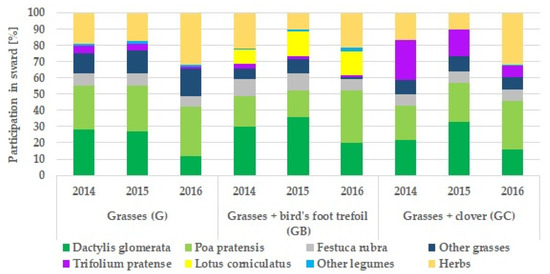
Figure 1.
The percentage of the dominant plant species in the three types of meadow sward (G, GB, GC) in study years (2014–2016).
2.3. Herbage Sampling and Analysis
Between 2014 and 2016 ten herbage samples were collected from each part of the meadow at seven-day intervals. Samples from an area of 1 m2 were hand-cut with scissors at the height of 5 cm. Every year, sampling started at the end of April and was continued until the end of June. Herbage samples were collected for chemical analyses and to determine the dry mass yield (DMY).
The DMY was assessed on the basis of the fresh weight of biomass collected from 1m2. The dry matter content was measured with the oven method (100 g of sample was dried in an oven for 24 h at a temperature of 105 °C) and expressed as tonnes of dry matter per hectare. The crude protein (CP) content in harvested herbage was used to calculate the crude protein yield (CPY). The DMY and CPY were expressed as tonnes per hectare.
The remainder of the sample was left for chemical analyses. After drying and grinding the samples, the crude protein content (CP) and dry matter digestibility (DMD) were estimated with the NIRS method on a NIRFlex N-500 near-infrared spectrometer (Büchi Labortechnik AG, Flawil, Switzerland) with ready-made INGOT® meadow hay calibrations.
2.4. Weather Conditions
Meteorological data were gathered from the Warsaw-Okęcie weather station (EPWA 12375) located approximately 4 km away from the research site. The Selyaninov hydrothermal coefficient (HTC) [64] was used for detailed assessment of rainfall and temperature in growing seasons (from March to June). The following formula was used for calculations:
where:
HTC = (P × 10)/Σt
P—total monthly rainfall (mm),
Σt—sum of monthly average daily air temperatures > 0 °C.
The available meteorological data were used to calculate the average daily temperature (T_AV), total rainfall (PREC_S), and cumulative degree-day values (T_S) for each date of herbage sampling. The date of the beginning of the growing season in each year was calculated from the average daily temperatures and the total rainfall according to the mathematical formula developed by Gumiński [65].
During the period under study, the weather conditions were diverse, especially the amount and distribution of rainfall (Figure 2). In the first year (2014), the amount and distribution of rainfall was favourable for plant growth. In 2015 April it was fairly humid, May was dry, and June was very dry. April and June were fairly dry in the third year, and May was very dry (Table 1).
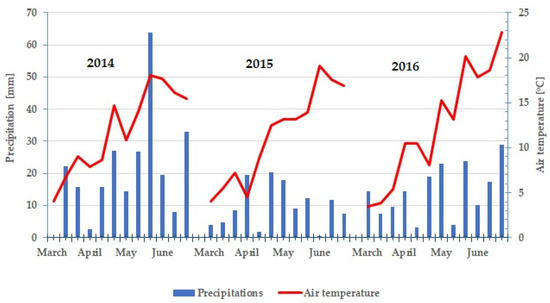
Figure 2.
Average decade air temperatures and precipitation in period March–June in study years (2014–2016).

Table 1.
Values of the Selyaninov hydrothermal coefficient (HTC).
2.5. Organisation and Division of Experimental Data
The first stage of work on the concept of the development of deterministic models involved the creation of a spreadsheet database, which contained all the data from the field experiment conducted between 2014 and 2016. In total, 840 experimental cases were collected. It is important to note that an experiment replicate was treated as a separate case. One of the research assumptions was not to include the cases with incomplete experimental information or with data raising objections in the final analyses. Figure 3 shows the concept of development of deterministic models based on the field experiment.
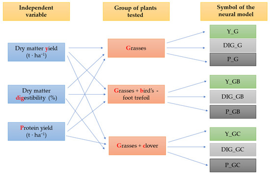
Figure 3.
The deterministic models developed in the study, including the independent variables and three experimental variants.
As shown in Figure 3, the authors of this study proposed the creation of nine deterministic models, differing in the output variable and the main factor from the field experiment. The following variables could be found at the network output in the models presented in the study: dry matter yield (t∙ha−1), dry matter digestibility (%), and protein yield (t∙ha−1). In addition, the experiment was diversified in terms of the species composition in the sward. The sward consisted of grasses (G), grasses and bird’s foot trefoil (GB), and grasses and red clover (GC). The adoption of the concept enabled the creation of the following deterministic models: Y-G—a yield model for the sward consisting mostly of grasses, DIG_G—a model of dry matter digestibility percentage for the sward consisting mostly of grasses, P_G—a protein yield model for the sward consisting mostly of grasses, Y-GB—a yield model for the sward consisting of grasses and bird’s foot trefoil, DIG_GB—a model of dry matter digestibility percentage for the sward consisting of grasses and bird’s foot trefoil, P_GB—a protein yield model for the sward consisting of grasses and bird’s foot trefoil, Y_GC—a yield model for the sward consisting of grasses and red clover, DIG_GC—a model of dry matter digestibility percentage for the sward consisting of grasses and red clover, and P_GC—a protein yield model for the sward consisting of grasses and red clover.
2.6. Deterministic Models—Construction Methodology
The deterministic models for the grassy sward (Y_G, DIG_G, and P_G), the sward with grasses and bird’s foot trefoil (Y_GB, DIG_GB, and P_GB), and the sward with grasses and clover (Y_GC, DIG_GC, and P_GC) were based on the same input variables (Table 2). The output variable was the differentiating factor.
Table 2.
The structure and ranges of data used for the construction of deterministic models, including the symbol of each variable.
Three types of factors represented the independent variables: phytophenological factors, meteorological factors, and factors related to the percentage share of various plant groups in the sward composition. The phytophenological variable, i.e., the harvest date (H_D), was expressed as the number of days since the beginning of the calendar year. The meteorological variables, i.e., the average daily temperature (T_AV), total rainfall (PREC_S), and total effective temperatures (T_S) in each year of the study were calculated for the period ranging from the spring onset of vegetation to the harvest date. The variables related to the percentage share of various groups of plants in the sward were calculated based on the botanical composition of the sward, which was determined in each year in mid-May. The output variables, i.e., the dry matter digestibility (%) (%_DMD), dry matter yield (t∙ha−1) (Y_DM), and protein yield (t∙ha−1) (P_Y) were determined in each year after the harvest.
It is difficult to choose the right architecture of neural networks due to their different specificity, the data selected for analysis and the selected learning method. Therefore, the generalisation and approximation abilities of networks based on previously established measures of their quality were taken into account when selecting the best topology and learning method.
Various network architectures were tested with the Automatic Network Designer implemented in the Statistica v7.1 software [66]. Ten thousand neural networks were tested for each of the issues under consideration. The analyses enabled the selection of the best neural network architecture. A multi-layer perceptron network with two hidden layers was selected for all models tested: Y_G, DIG_G, P_G, Y_GB, DIG_GB, P_GB, Y_GC, DIG_GC, and P_GC. This type of network is often used to implement prognostic and deterministic issues in agricultural production [43,67]. When selecting the networks that will be used at further stages of the analyses, the best values of parameters relating to their quality were taken into account, i.e., standard error deviation, mean value of error modules, standard deviation quotient, and correlation coefficient. If the results were ambiguous or difficult to assess, networks with a high correlation coefficient and a low value of the mean absolute error were searched. Table 3 lists the structures of selected neural networks.
Table 3.
The structures of neural networks in the deterministic models and the learning methods.
To train and verify the selected multilayer perceptron networks, each data set containing experimental cases, were randomly divided into three sets: training set (70% of cases), validation set (15% of cases), and test set (15% of cases). The data collected in the training set enabled the calculation of the gradient, weight, and value of all loads for the network. The isolation of the validation set made it possible to monitor the network learning error during the learning stage continuously. If the error of the validation set tended to increase for several consecutive epochs, the learning process was stopped. In general, this set is attributed a very important role—it prevents the overlearning of the neural network. The test set was intended to carry out a one-time verification and control after the completion of learning to check whether, despite periodic validation, the neural network had not lost the generalisation ability.
Two neural network learning methods were used: backward propagation of errors (BP) and conjugate gradient method (CG). The results listed in Table 3 show that there were different conditions at the end of the network learning process. All the networks were trained with the backpropagation method for 100 epochs. The learning with the conjugate gradient method was diversified. The learning of the MLP 7:7-11-5-1:1 network in the Y_G model was the shortest at the second stage—57 epochs. The learning of the MLP 7:7-9-5-1:1 network in the P_GC model was the most time-consuming—it took 113 learning cycles with the conjugate gradient method.
2.7. Neural Networks—Sensitivity Analysis
After learning the neural network, its sensitivity was analysed to show which input data were the most important in explaining the variability of the dependent variable. This information was obtained by analysing the increase in error while eliminating individual variables from the input data. This task is accomplished by using the error quotient represented by the rank used. The error quotient expresses the ratio of the error to the total error of all independent variables. As its value increases, so does the significance of a particular variable. If the quotient value is below 1 for any of the independent variables, it is best to remove it from the model to improve its quality. The rank shows the position of the variable on the “ranking list”—it indicates the characteristics according to the decreasing error. The rank value of 1 means that this variable contributed the most to the explanation of variability of the dependent variable [44,68,69].
3. Results
3.1. Neural Network Sensitivity Analysis—Summary
Table 4 shows the results of the analysis of sensitivity of neural networks in the Y_G, DIG_G, P_G, Y_GB, DIG_GB, P_GB, Y_GC, DIG_GC, and P_GC models for three variables ranked from 1 to 3. The corresponding values of the error quotients were considered.
Table 4.
The results of the neural networks sensitivity analysis in the Y_G, DIG_G, P_G, Y_GB, DIG_GB, P_GB, Y_GC, DIG_GC, and P_GC models.
Data in Table 4 shows that the average daily air temperature (T_AV), calculated for the period ranging from the spring onset of vegetation to the harvest date, was the independent variable with the greatest influence on the values of most of the tested dependent variables. Other important rank one variables were: the total rainfall (P_GB model) and the percentage of legumes in the sward (%_L). Rank two2 in the analysis of the sensitivity of neural networks was most often assumed by the independent variable T_S, i.e., the total temperatures in the period ranging from the spring onset of vegetation to the harvest date. The other rank two variables were the harvest date (H_D) in the Y_GB model and the total rainfall (PREC_S) in the P_GC model. Rank three in all the models was diversified. It was assigned four times to the total rainfall variable (PREC_S) in nine models. The variable referring to the percentage share of legumes in the sward (%_L) was identified twice. It is noteworthy that in each of the analyses the significance of all tested variables was confirmed—the value of the quotient was above one for each variable.
3.2. Response Charts for the Most Significant Variables
Response charts show how the predicted value changes as a function of the selected independent variable. The comparison of the response charts with the ranks provided by the sensitivity analysis shows which parameters, and to what extent, influence the value of the dependent variable. Figure 4, Figure 5, Figure 6, Figure 7, Figure 8, Figure 9, Figure 10, Figure 11 and Figure 12 show the relations between the rank one variables from the neural network sensitivity analyses and the values of the dependent variables for the Y_G, DIG_G, P_G, Y_GB, DIG_GB, P_GB, Y_GC, DIG_GC, and P_GC models.
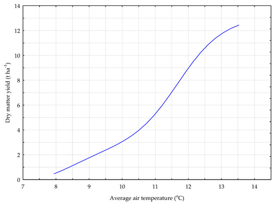
Figure 4.
The Y_G model. The response chart for variables T_AV (rank 1) and Y_DM.
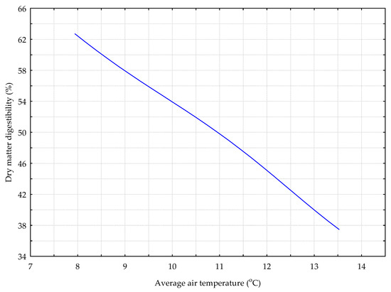
Figure 5.
The DIG_G model. The response chart for variables T_AV (rank 1) and %_DMD.
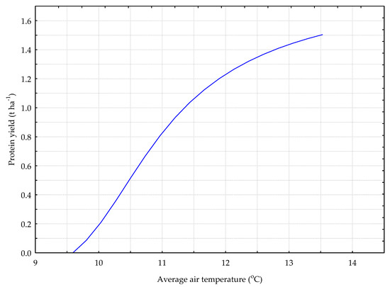
Figure 6.
The P_G model. The response chart for variables T_AV (rank 1) and P_Y.
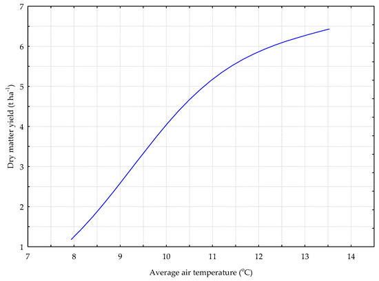
Figure 7.
The Y_GB model. The response chart for variables T_AV (rank 1) and Y_DM.
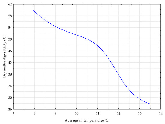
Figure 8.
The DIG_GB model. The response chart for variables T_AV (rank 1) and %_DMD.
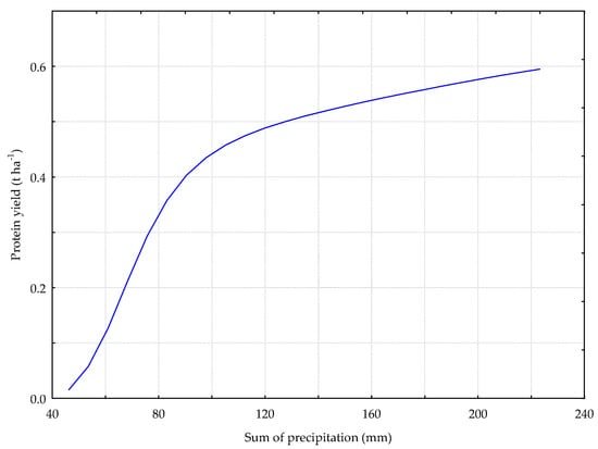
Figure 9.
The P_GB model. The response chart for variables PREC_S (rank 1) and P_Y.
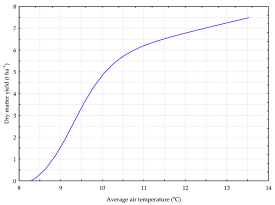
Figure 10.
The Y_GC model. The response chart for variables T_AV (rank 1) and Y_DM.
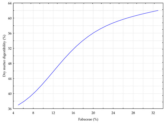
Figure 11.
The DIG_GC model. The response chart for variables %_L (rank 1) and %_DMD.
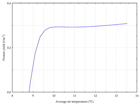
Figure 12.
The P_GC model. The response chart for variables T_AV (rank 1) and P_Y.
In the deterministic model for the grass sward (Y_G) shown in Figure 4, the dry matter yield increased along with the average daily air temperature.
The data presented on Figure 5 show that an increase in the average daily air temperature caused a decrease in the digestibility of the dry matter of grass sward (%).
As the average daily air temperature increased, so did the yield of protein from the grass sward (Figure 6).
Figure 7 shows the relation between the yield of dry matter from the sward with the predominance of grasses and bird’s foot trefoil (Y_GB model) and the average daily air temperature (T_AV). The average daily air temperature in the period ranging from the spring onset of vegetation to the harvest date was the factor with the greatest influence on the yield of dry matter of green forage. As the value of this parameter increased, so did the value of the dependent variable.
The dependence between the percentage of digestibility of the dry matter from the sward with the predominance of grasses and bird’s foot trefoil and the two variables with the greatest influence on explaining the variability of this trait (DIG_GB model) is presented on Figure 8. An increase in the average daily air temperature caused a decrease in the dry matter digestibility.
Figure 9 shows the relation between the yield of protein from the sward with the predominance of grasses and bird’s foot trefoil and the total rainfall in the test period (PREC_S). As seen from the data, the higher the rainfall in the period ranging from the spring onset of vegetation to the harvest date was, the higher the yield of protein from the harvested biomass was.
The relation between the yield of dry matter from the sward with the predominance of grasses and red clover (Y_GB model) and the average daily air temperature (T_AV) is shown on Figure 10. The average daily air temperature in the period ranging from the spring onset of vegetation to the harvest date stimulated the yield of dry matter from the sward with the predominance of grasses and red clover.
Figure 11 shows the data referring to the dependence between the percentage of digestibility of the dry matter from the sward with the predominance of grasses and red clover (DIG_GC model). An increase in the percentage share of legumes (%_L) caused an increase in the digestibility of the green forage dry matter.
The relation between the average daily air temperature (T_AV)—rank one and the protein yield is presented on Figure 12. An increase in the average daily air temperature to about 9.5 °C stimulated the accumulation of protein in the sward with the predominance of grasses and red clover. When this value was exceeded, the protein yield remained at a steady level of about 0.3 t∙ha−1.
3.3. Comparison of Qualitative Parameters of Generated Models
In each of the presented cases, all the deterministic models were characterised by the best values of the measures referring to the quality of the generated neural networks (Table 5). When it was difficult to identify the best network at the summary stage, the values of two qualitative parameters were taken into account: the correlation coefficient (r) and the mean absolute error. The authors followed the principle that the value of the correlation coefficient was to be the highest, whereas the value of the mean absolute error was to be low. In the nine cases under analysis the values of the correlation coefficient were high or very high, as they ranged from 0.739 (P_GB model) to 0.946 (DIG_GB model). The value of the mean absolute error was the lowest for the P_G model—it amounted to 0.094 t∙ha−1. The highest value of the mean absolute error was noted for the DIG_GC model—3.584%. The error quotient was another important parameter of assessment of the quality of the neural networks. It was defined as the quotient of the standard deviation of the prediction errors and the standard deviation of the output variable. The value of this parameter should not exceed 0.7 for the model to be useful for prognostic purposes. Each of the nine cases under analysis met this assumption. The lowest value of the deviation quotient was noted for the DIG_GB model—0.321.
Table 5.
The values of the main qualitative parameters for the neural networks in the tested models.
4. Discussion
Over the past decades, many models describing grass growth have been developed. They have ranged from simple empirical models [70,71] to more complex mechanistic models [72,73,74]. They are often based on growth, senescence, litter, and standing biomass. They use data on incoming radiation, temperature, soil moisture, day length, and altitude. The development of grass growth models in response to temperature may help to forecast the growth depending on the season and temperature and show how climate change affects grassland productivity [31]. Climate changes, which are also noticeable in Poland, lead to the systematic deterioration of humidity conditions. Particularly grasslands are sensitive to fluctuations in climatic conditions. Rising temperatures and rainfall deficits will cause changes in the species composition of grasslands, their productivity [37,38,39] and, consequently, in the quality of obtained forages. User-friendly grass growth prediction models provide real-time information based on forecasted meteorological data and farm management data to predict grass growth. Hence, herbage supply may allow farmers to manage a key resource on their farms.
These models facilitate a better understanding of the grass growth processes and their interactions with farm management. They also help to study the influence of the environment on grassland. Grass growth models are often sub-models or elements of larger farm system models, e.g., in APSIM [75], PaSim [76,77], EcoMod, DairyMod, and the SGS pasture model [74]. Integrated models can be used to assess the effects of climate change on grasslands production and livestock production systems. For example, the PaSim model was used to assess the effects of climate change on the productivity pastures and ruminants. It is important to assess models to make sure that the selected model can be used in a specific region or under specific conditions [78].
In our study, the average daily air temperature calculated for the period ranging from the spring onset of vegetation to the harvest date was the independent variable with the greatest influence on the values of most of the tested dependent variables. In all the deterministic models, the dry matter yield tended to increase along with the average daily air temperature. However, this increase was curvilinear and reached the maximum values when temperatures exceeded 10 °C. This is consistent with other scientific reports, according to which the grass growth rate is controlled by three factors: temperature, soil moisture content, and the intensity of sunlight. Of these three factors, it is temperature that has the greatest influence on the grass growth rate, especially in the spring, because it determines the rate of plant development and the structure of the root mass and aerial parts of plants [14,79]. In Poland, the grass growing season is assumed to begin when the average daily air temperature exceeds 5 °C for five consecutive days [80]. Depending on the region and the year, this moment may occur as early as the beginning of March. Taking the temperature above 5 °C as the starting point, the higher the temperature, the faster the sward growth rate is until the temperature is about 10 °C [81,82]. Most grass species achieve the maximum growth rate at an average daily temperature of about 10 °C. A further increase in temperature has little influence on the growth rate of grassland plants. Therefore, the temperature range of 10–15 °C is considered to be optimal for the good development and yield of grassland sward.
Air temperature affects the intensity of intracellular metabolic processes during plant growth. It causes changes in the chemical composition of plants, mainly in the formation of structural carbohydrates, such as hemicellulose, cellulose, and lignin, which influence the digestibility of feed [71,83]. In our study, the average daily temperature also influenced the digestibility of the dry matter of grasses (DIG_G model) and grasses with bird’s foot trefoil (DIG_GB). There was a rectilinear decrease in the digestibility of dry matter observed along with an increase in the average daily temperature calculated from the vegetation onset to the harvest day. A similar phenomenon was observed by Żurek [84], who analysed the relationship between the digestibility of the dry matter of rescuegrass (Bromus willdenowii) and tall fescue (Festuca arundinacea) and the average daily air temperature during the growing season in Poland. Like in our study, the digestibility of the dry matter of both grass species tended to decrease as the average daily air temperature increased. The average daily temperature also influenced the yield of protein from the grass sward (P_G model) and the grass and red clover sward (P_GC). The protein yield, being the resultant of the dry matter yield and protein content in the harvested crops, increased along with the average daily temperature in both cases. However, there were differences in this increase influenced by the sward species composition. The fastest increase in the protein yield in the grass sward was observed at 10–13 °C, which is the optimal temperature range for grasses. In the grass and clover sward, the most intense increase in the protein yield was observed within a very narrow range of temperatures, i.e., 8.5–9.5 °C. There was no increase in the protein yield at temperatures higher than 9.5 °C.
It is a well-known fact that grassland productivity and rainfall are often positively correlated with each other [85,86]. In our study the total rainfall assumed rank one only in the model of the yield of protein from the sward with grass and bird’s foot trefoil (P_GB). As the amount of rainfall increased, so did the protein yield. The total rainfall was the least significant (rank three) variable for the yield models of all three types of sward (Y_G, Y_GB, and Y_GC) and the model of digestibility of grasses with bird’s foot trefoil (DIG_GB). The insignificant or poorly significant influence of rainfall on the yield of all types of sward may have been caused by the fact that plants use water stored in the soil in autumn and winter to produce the first regrowth in spring, so the lack of rainfall in this period does not limit the growth of the sward. On the other hand, a low soil moisture content in summer disrupts the photosynthesis and transpiration processes, thus limiting the development of plants and their yield [41,87]. Grasses, which predominate in the composition of sward with a mixture of legumes and grasses in the spring regrowth, have a special ability to make good use of the water resources accumulated during the winter. In summer with periodic rainfall deficiencies, legumes predominate in the regrowth, because, unlike grasses, they better withstand periodic and short-term summer droughts [88]. During longer periods of drought, which sometimes occur in the middle of summer, plant growth is completely inhibited. For example, in summer, when the amount of rainfall was insufficient, the yield of red clover decreased by 3–34%, as compared with the yield obtained under the optimal soil moisture content with a rainfall of 350–460 mm [89].
Another important rank one variable was the percentage of legumes in the sward (%_L). The digestibility of dry matter in the sward tended to increase along with the percentage share of red clover (Trifolium pratense) in the DIG_GC deterministic model. Earlier studies showed that the presence of red clover in the sward positively affected the digestibility of feed and its protein content [90,91]. The share of legumes in mixtures with grasses increases the feed energy and protein content, contributes to more efficient absorption of these nutrients in the digestive system, and thus influences the growth of animals receiving these feeds [92,93]. Moreover, the sward composed of red clover and bird’s foot trefoil with grasses enriches the feed with vitamins, fatty acids, and carotene [94,95]. According to an earlier study [96], the best chemical composition and the highest nutritional value of grass and clover mixtures is obtained when the share of red clover in the yield is 50%. According to Staniak [97], mixtures with 60% and 80% clover content were the best balanced in terms of the protein and fibre content. In the study by Wróbel and Zielewicz [90], the optimal content of protein was guaranteed by a 30–40% share of bird’s foot trefoil and a 60–80% share of red clover. Our study showed that a higher share of legumes resulted in a higher digestibility of the sward. A 5% share of legumes in the sward resulted in the dry matter digestibility of 37–38%. However, when the share of legumes in the sward increased to 33%, the digestibility of the feed increased to 62%.
The development of plants (the sequence of consecutive development phases) depends almost exclusively on temperature and the length of the day. Therefore, one of the most popular units used in agriculture for measurements of plant growth, development, and maturity is the growing degree-day (GDD), which ensures a more accurate physiological estimate than calendar days alone [98]. The GDD is a measure of heat accumulation above a certain base temperature, which is different for each forage species. When days are warmer than those marked as normal for a particular species, plants grow rapidly. However, when temperature drops below the base level, the GDD value does not increase. The GDD is an important measure determining the dynamics of plant development because each development stage requires a specific amount of accumulated sum of GDD temperatures.
The sum of temperatures determines the length of plants’ growing seasons, stimulates individual stages of their growth and development, and the actual production of dry matter, including the occurrence of critical periods of temperature stress [99]. In our study, total temperatures (T_S) was a rank two parameter in the analysis of the sensitivity of neural networks. The increase in total temperatures resulted in a decrease in the protein content in the sward.
GDD is a value that enables an approximate prediction of the dates when individual plant development phases will begin. However, due to climate change the total GDD may increase, whereas the number of days necessary for crops to mature may decrease and this may accelerate the sward harvest date. This may mean that due to an earlier occurrence of the necessary sum of temperatures, individual plant species will grow faster. In consequence, the sward will have to be mown and forage will have to be harvested much earlier than in other years [100,101].
The harvest date (H_D), expressed as the number of days from the beginning of the calendar year, was a significant parameter only in the model of the yield from the sward with grasses and bird’s foot trefoil (Y_GB model), where it assumed rank two (Table 3). The lack of proven significance of this variable means that this parameter should not be taken into account in the construction of grassland sward yield models. The lack of significance of this variable in most models results from the considerable variability of the course of meteorological conditions in individual growing seasons, mainly rainfall and total temperatures, which have the greatest influence on the quantitative and qualitative changes in the biomass of various plants grown in fields and grasslands [102,103].
Artificial neural networks are a suitable tool for making deterministic models, which can be used in plant production, including grassland production. The right rendering of the results generated by a model makes it possible to explain the influence of a significant factor on the dependent variable.
The choice of the right network topology and learning method is one of the key steps in working with neural networks. These parameters are closely related to the target use of this model. There are usually differences between networks selected for typical classification problems and those for prognostic and deterministic problems. In this paper the authors of neural models usually use available scientific publications discussing similar research topics, but it is one’s own experience in working with neural models and the knowledge of the research object that should be the main guidelines for finding the optimal approach to presenting and solving the problem. In our study, an MLP network with two hidden layers was finally selected.
Neural network learning makes it possible to combine certain behaviours of the model based on multiple learning cases. The model user enforces specific responses to the given input signals from the network. The network remembers the questions and responses based on learnt patterns of behaviour to provide the closest response to the original when the next question is asked. All the neural networks presented in our study were trained in two stages. The error backpropagation method was used at the first stage of the process. Each time this process was continued for 100 epochs. The learning was continued thanks to the inclusion of the conjugate gradient method. The best result of network learning was obtained after a different number of learning cycles. Thanks to this dual approach to learning it is possible to create neural networks with very favourable qualitative parameters [44,104].
The selected neural networks used as the bases for the creation of nine models: Y_G, DIG_G, P_G, Y_GB, DIG_GB, P_GB, Y_GC, DIG_GC, and P_GC, had very favourable values of qualitative parameters. The MLP 7:7-11-8-1:1 network fared particularly well—the value of the correlation coefficient was close to one, whereas the value of the deviation quotient was 0.324. These results show that the network was very well suited to the set of cases used for its construction. This proves the high reliability of analyses. The collective analysis of the values of the qualitative parameters assumed by the tested models leads to the conclusion that each of these models has a high application potential [105].
The selection of independent variables for the construction of a deterministic model is a compromise between the experimental dataset, the author’s practical knowledge, and the requirements of the market and potential users of the model. It is important to remember that the choice of variables must enable real influence on the dependent variable and that variables must be freely accessible. Although the significance of selected variables can be checked by means of additional analyses and calculations [106], practical experience is the best way to properly adjust the independent variables to explain the complexity and variability of a particular phenomenon. Additional software gathering experimental data used in the model significantly reduces its application capability. Our study used meteorological data (T_AV, PREC_S, and T_S), phytophenological data (H_D), and data on the share of individual groups of plants in the sward (%_G, %_L, and %_HW). Each of the nine models was based on the same independent variables, defined separately for each of the three types of sward: with the predominance of grasses, with grasses and bird’s foot trefoil, and with grasses and red clover.
The analysis of the sensitivity of neural networks enabled such a detailed approach to the explanation of the influence of the weather conditions (temperature and rainfall) in the spring on the dry matter yield of the harvested plant biomass and its quality. This method enables the distinction between significant variables in the model and those that have little influence on the result of the network operation [107]. This method is widely used to select the most important variables for problems related to the phenology and yield of crop species [108,109,110]. The presentation of the relations (Figure 4, Figure 5, Figure 6, Figure 7, Figure 8, Figure 9, Figure 10, Figure 11 and Figure 12) between the variables with the greatest influence on the explanation of variability of the dependent variables and the dependent variables themselves gives a chance for efficient and conscious control of plant production in the current crop growing season. It is an excellent basis for the implementation of a wide range of practical recommendations concerning agricultural production.
5. Conclusions
The pilot study presented in this paper included the successive steps of field and climate data acquisition from a 3-year study, the construction of neural networks and their sensitivity analysis, and the generation of network response plots. An important element of inference was the generation of nine neural models for which the inputs were seven independent traits, i.e., harvest date, mean daily temperature, total precipitation, total effective temperature, and the proportion of grasses, broad beans, herbs, and weeds in the sward. The output of the network included the following attributes: dry matter yield, dry matter digestibility, and protein yield. The obtained results of the analyses lead to the following conclusions:
- The deterministic models developed and verified in our experiment enabled the implementation of the aim of the study set in this paper. This means that artificial neural networks can be used to pre-identify highly significant factors affecting the yield and digestibility of grassland sward in the climatic conditions of central Poland.
- The analysis of the sensitivity of a neural network enables the preliminary selection of factors with the greatest influence on the dependent (output) variable, while maintaining the assumed level of significance.
- The average daily air temperature (T_AV) is usually the factor with the greatest influence on the tested output variables: dry matter digestibility, dry matter yield, and protein yield, regardless of the species composition of the sward. The total rainfall (PREC_S) and the percentage of legumes were also significant factors.
- Future research on the improvement of deterministic models in grassland production should concentrate on several aspects. First, it is necessary to analyse in detail the influence of other equally important independent variables, which are usually expressed in a linguistic form. Second, other analytical methods enabling the optimization of significant (controllable) production factors should also be used, because they considerably affect the quality and quantity of the yield of grassland sward.
Author Contributions
Conceptualization, G.N., B.W. and M.P.; methodology, G.N., B.W., M.P., W.Z. and A.P.-J.; software, G.N., B.W., T.W. and M.N.; validation, G.N., B.W., M.P., W.Z. and A.P.-J.; formal analysis, G.N., B.W., M.P., W.Z., A.P.-J. and T.W.; investigation, B.W.; resources, G.N., B.W., M.P., W.Z. and A.P.-J.; data curation, G.N., B.W., M.P., T.W. and M.N.; writing—original draft preparation, G.N., B.W., M.P., W.Z. and A.P.-J.; writing—review and editing, G.N., B.W., M.P., W.Z., A.P.-J., T.W. and M.N.; visualization, G.N., B.W. and M.P.; supervision, G.N. and B.W.; project administration, G.N.; funding acquisition, G.N., M.P., T.W. and M.N. All authors have read and agreed to the published version of the manuscript.
Funding
This research received no external funding.
Institutional Review Board Statement
Not applicable.
Informed Consent Statement
Not applicable.
Data Availability Statement
Not applicable.
Conflicts of Interest
The authors declare no conflict of interest.
References
- Hopkins, A.; Wilkins, R.J. Temperate grassland: Key developments in the last century and future perspectives. J. Agric. Sci. 2006, 144, 503–523. [Google Scholar] [CrossRef]
- O’Mara, F.P. The role of grasslands in food security and climate change. Ann. Bot. 2012, 110, 1263–1270. [Google Scholar] [CrossRef] [Green Version]
- Eurostat Overview—Agriculture-Eurostat. Available online: https://ec.europa.eu/eurostat/web/agriculture/overview (accessed on 27 October 2021).
- Statistics Poland. Production of agricultural and horticultural crops in 2019. Available online: https://stat.gov.pl/files/gfx/portalinformacyjny/pl/defaultaktualnosci/5509/9/18/1/produkcja_upraw_rolnych_i_ogrodniczych_w_2019_r..pdf (accessed on 6 January 2022).
- Olesen, J.E.; Bindi, M. Consequences of climate change for European agricultural productivity, land use and policy. Eur. J. Agron. 2002, 16, 239–262. [Google Scholar] [CrossRef]
- Bengtsson, J.; Bullock, J.M.; Egoh, B.; Everson, C.; Everson, T.; O’Connor, T.; O’Farrell, P.J.; Smith, H.G.; Lindborg, R. Grasslands—More important for ecosystem services than you might think. Ecosphere 2019, 10, e02582. [Google Scholar] [CrossRef]
- Sollenberger, L.E.; Kohmann, M.M.; Dubeux, J.C.B.; Silveira, M.L. Grassland management affects delivery of regulating and supporting ecosystem services. Crop Sci. 2019, 59, 441–459. [Google Scholar] [CrossRef]
- Zhao, Y.; Liu, Z.; Wu, J. Grassland ecosystem services: A systematic review of research advances and future directions. Landsc. Ecol. 2020, 35, 793–814. [Google Scholar] [CrossRef]
- Gabryszuk, M.; Barszczewski, J.; Wróbel, B. Characteristics of grasslands and their use in Poland. J. Water L. Dev. 2021, 51, 243–249. [Google Scholar] [CrossRef]
- Gibon, A. Managing grassland for production, the environment and the landscape. Challenges at the farm and the landscape level. Livest. Prod. Sci. 2005, 96, 11–31. [Google Scholar] [CrossRef]
- Paszkiewicz-Jasińska, A.; Steinhoff-Wrześniewska, A. Natural and landscape values of distinguished meadow-pasture communities in Kłodzko country. J. Res. Appl. Agric. Eng. 2017, 62, 75–80. [Google Scholar]
- Boval, M.; Dixon, R.M. The importance of grasslands for animal production and other functions: A review on management and methodological progress in the tropics. Animal 2012, 6, 748–762. [Google Scholar] [CrossRef] [Green Version]
- Yates, S.; Jaškūnė, K.; Liebisch, F.; Nagelmüller, S.; Kirchgessner, N.; Kölliker, R.; Walter, A.; Brazauskas, G.; Studer, B. Phenotyping a dynamic trait: Leaf growth of perennial ryegrass under water limiting conditions. Front. Plant Sci. 2019, 10, 344. [Google Scholar] [CrossRef]
- Wingler, A.; Hennessy, D. Limitation of grassland productivity by low temperature and seasonality of growth. Front. Plant Sci. 2016, 7, 1130. [Google Scholar] [CrossRef] [Green Version]
- Chang, J.; Viovy, N.; Vuichard, N.; Ciais, P.; Campioli, M.; Klumpp, K.; Martin, R.; Leip, A.; Soussana, J.F. Modeled changes in potential grassland productivity and in grass-fed ruminant livestock density in Europe over 1961–2010. PLoS ONE 2015, 10, e0127554. [Google Scholar] [CrossRef] [Green Version]
- Zielewicz, W.; Swędrzyński, A.; Dobrzyński, J.; Swędrzyńska, D.; Kulkova, I.; Wierzchowski, P.; Wróbel, B. Effect of forage plant mixture and biostimulants application on the yield, changes of botanical composition, and microbiological soil activity. Agron. 2021, 11, 1786. [Google Scholar] [CrossRef]
- Pelletier, S.; Tremblay, G.F.; Bélanger, G.; Bertrand, A.; Castonguay, Y.; Pageau, D.; Drapeau, R. Forage nonstructural carbohydrates and nutritive value as affected by time of cutting and species. Agron. J. 2010, 102, 1388–1398. [Google Scholar] [CrossRef]
- Poetsch, E.; Resch, R.; Krautzer, B. Variability of forage quality between and within three maturity groups of Lolium perenne L. during the first growth. Grassl. Sci. Eur. 2016, 21, 293–295. [Google Scholar]
- Rinne, M.; Nykänen, A. Timing of primary growth harvest affects the yield and nutritive value of timothy-red clover mixtures. Agric. Food Sci. Finl. 2000, 9, 121–134. [Google Scholar] [CrossRef]
- Capstaff, N.M.; Miller, A.J. Improving the yield and nutritional quality of forage crops. Front. Plant Sci. 2018, 9, 535. [Google Scholar] [CrossRef] [Green Version]
- Lee, M.A. A global comparison of the nutritive values of forage plants grown in contrasting environments. J. Plant Res. 2018, 131, 641–654. [Google Scholar] [CrossRef]
- Cantarel, A.A.M.; Bloor, J.M.G.; Soussana, J.-F. Four years of simulated climate change reduces above-ground productivity and alters functional diversity in a grassland ecosystem. J. Veg. Sci. 2013, 24, 113–126. [Google Scholar] [CrossRef]
- Hoffstätter-Müncheberg, M.; Merten, M.; Isselstein, J.; Kayser, M.; Wrage-Mönnig, N. Drought effects on herbage production of permanent grasslands in northern Germany. Grassl. Sci. Eur. 2014, 19, 106–108. [Google Scholar]
- Huyghe, C.; de Vliegher, A.; van Gils, B.; Peeters, A. Grasslands and Herbivore Production in Europe and Effects of Common Policies; Quae Editions: Versailles, France, 2014. [Google Scholar]
- Joyce, C.B. Ecological consequences and restoration potential of abandoned wet grasslands. Ecol. Eng. 2014, 66, 91–102. [Google Scholar] [CrossRef]
- Smit, H.J.; Metzger, M.J.; Ewert, F. Spatial distribution of grassland productivity and land use in Europe. Agric. Syst. 2008, 98, 208–219. [Google Scholar] [CrossRef]
- Kipling, R.P.; Bannink, A.; Bellocchi, G.; Dalgaard, T.; Fox, N.J.; Hutchings, N.J.; Kjeldsen, C.; Lacetera, N.; Sinabell, F.; Topp, C.F.E.; et al. Modeling European ruminant production systems: Facing the challenges of climate change. Agric. Syst. 2016, 147, 24–37. [Google Scholar] [CrossRef] [Green Version]
- Anders, I.; Stagl, J.; Auer, I.; Pavlik, D. Climate change in central and eastern Europe. In Managing Protected Areas in Central and Eastern Europe under Climate Change; Springer: Berlin/Heidelberg, Germany, 2014; Volume 58, pp. 17–30. [Google Scholar]
- Trnka, M.; Olesen, J.E.; Kersebaum, K.C.; Skjelvåg, A.O.; Eitzinger, J.; Seguin, B.; Peltonen-Sainio, P.; Rötter, R.; Iglesias, A.; Orlandini, S.; et al. Agroclimatic conditions in Europe under climate change. Glob. Chang. Biol. 2011, 17, 2298–2318. [Google Scholar] [CrossRef] [Green Version]
- Raich, J.W.; Tufekciogul, A. Vegetation and soil respiration: Correlations and controls. Biogeochemistry 2000, 48, 71–90. [Google Scholar] [CrossRef]
- Höglind, M.; Thorsen, S.; Semenov, M. Assessing Uncertainties in Impact of Climate Change on Grass Production in Northern Europe Using Ensembles of Global Climate Models; Elsevier: Amsterdam, The Netherlands, 2013; Volume 170, pp. 103–113. [Google Scholar]
- Van Oijen, M.; Balkovi, J.; Beer, C.; Cameron, D.R.; Ciais, P.; Cramer, W.; Kato, T.; Kuhnert, M.; Martin, R.; Myneni, R.; et al. Impact of droughts on the carbon cycle in European vegetation: A probabilistic risk analysis using six vegetation models. Biogeosciences 2014, 11, 6357–6375. [Google Scholar] [CrossRef] [Green Version]
- Thumm, U.; Tonn, B. Effect of precipitation on dry matter production of a meadow with varied cutting frequency. Grassl. Sci. Eur. 2010, 15, 90–92. [Google Scholar]
- Li, Q.; Hou, J.; Yan, P.; Xu, L.; Chen, Z.; Yang, H.; He, N. Regional response of grassland productivity to changing environment conditions influenced by limiting factors. PLoS ONE 2020, 15, e0240238. [Google Scholar] [CrossRef]
- Łabędzki, L. Actions and measures for mitigation drought and water scarcity in agriculture. J. Water L. Dev. 2016, 29, 3–10. [Google Scholar] [CrossRef] [Green Version]
- Kaca, E.; Łabędzki, L.; Lubbe, I. Gospodarowanie wodą w rolnictwie w obliczu ekstremalnych zjawisk pogodowych. Postępy Nauk Rol. 2011, 1, 37–49. [Google Scholar]
- Goliński, P.; Czerwiński, M.; Jørgensen, M.; Mølmann, J.A.B.; Golińska, B.; Taff, G. Relationship between climate trends and grassland yield across contrasting European locations. Open Life Sci. 2018, 13, 589–598. [Google Scholar] [CrossRef]
- Goliński, P.; Czerwinski, M.; Golińska, B. Effect of climate change in 50-years period on grassland productivity in central Poland. In Sustainable Use of Grassland Resources for Forage Production, Biodiversity and Environmental Protection, International Grassland Congress; Roy, A.K., Kumar, R.V., Agrawal, R.K., Mahanta, S.K., Singh, J.B., Das, M.M., Al, E., Eds.; Rangeland Management Society of India: New Delhi, India, 2015; pp. 9–286. [Google Scholar]
- Knapp, A.; Smith, M. Variation among biomes in temporal dynamics of aboveground primary production. Science 2001, 291, 481–484. [Google Scholar] [CrossRef] [Green Version]
- Hlavinka, P.; Trnka, M.; Semerádová, D.; Dubrovský, M.; Žalud, Z.; Možný, M. Effect of drought on yield variability of key crops in Czech Republic. Agric. For. Meteorol. 2009, 149, 431–442. [Google Scholar] [CrossRef]
- Staniak, M.; Kocoń, A. Forage grasses under drought stress in conditions of Poland. Acta Physiol. Plant. 2015, 37, 116. [Google Scholar] [CrossRef] [Green Version]
- Čimo, J.; Šinka, K.; Tárník, A.; Aydin, E.; Kišš, V.; Toková, L. Impact of climate change on vegetation period of basic species of vegetables in Slovakia. J. Water L. Dev. 2020, 47, 38–46. [Google Scholar] [CrossRef]
- Hara, P.; Piekutowska, M.; Niedbała, G. Selection of independent variables for crop yield prediction using artificial neural network models with remote sensing data. Land 2021, 10, 609. [Google Scholar] [CrossRef]
- Piekutowska, M.; Niedbała, G.; Piskier, T.; Lenartowicz, T.; Pilarski, K.; Wojciechowski, T.; Pilarska, A.A.; Czechowska-Kosacka, A. The application of multiple linear regression and artificial neural network models for yield prediction of very early potato cultivars before harvest. Agronomy 2021, 11, 885. [Google Scholar] [CrossRef]
- Niedbała, G. Simple model based on artificial neural network for early prediction and simulation winter rapeseed yield. J. Integr. Agric. 2019, 18, 54–61. [Google Scholar] [CrossRef] [Green Version]
- Kujawa, S.; Dach, J.; Kozłowski, R.J.; Przybył, K.; Niedbała, G.; Mueller, W.; Tomczak, R.J.; Zaborowicz, M.; Koszela, K. Maturity classification for sewage sludge composted with rapeseed straw using neural image analysis. In Proceedings of the SPIE—Eighth International Conference on Digital Image Processing (ICDIP 2016), Chengu, China, 20–22 May 2016; Volume 10033, p. 100332H. [Google Scholar] [CrossRef]
- Wojciechowski, T.; Niedbala, G.; Czechlowski, M.; Nawrocka, J.R.; Piechnik, L.; Niemann, J. Rapeseed seeds quality classification with usage of VIS-NIR fiber optic probe and artificial neural networks. In Proceedings of the 2016 International Conference on Optoelectronics and Image Processing, ICOIP, Warsaw, Poland, 10–12 June 2016. [Google Scholar] [CrossRef]
- Li, Y.; Chao, X. ANN-based continual classification in agriculture. Agriculture 2020, 10, 178. [Google Scholar] [CrossRef]
- Walczak, S. Artificial neural networks. In Advanced Methodologies and Technologies in Artificial Intelligence, Computer Simulation, and Human-Computer Interaction; IGI Global: Hershey, PA, USA, 2019; pp. 40–53. [Google Scholar]
- Khoshroo, A.; Emrouznejad, A.; Ghaffarizadeh, A.; Kasraei, M.; Omid, M. Sensitivity analysis of energy inputs in crop production using artificial neural networks. J. Clean. Prod. 2018, 197, 992–998. [Google Scholar] [CrossRef]
- Heskes, T.M.; Kappen, B. Learning processes in neural networks. Phys. Rev. A 1991, 44, 2718–2726. [Google Scholar] [CrossRef] [PubMed] [Green Version]
- Tu, J.V. Advantages and disadvantages of using artificial neural networks versus logistic regression for predicting medical outcomes. J. Clin. Epidemiol. 1996, 49, 1225–1231. [Google Scholar] [CrossRef]
- Tan, S.S.; Smeins, F.E. Predicting grassland community changes with an artificial neural network model. Ecol. Modell. 1996, 84, 91–97. [Google Scholar] [CrossRef]
- Majkovič, D.; O’Kiely, P.; Kramberger, B.; Vračko, M.; Turk, J.; Pažek, K.; Rozman, Č. Comparison of using regression modeling and an artificial neural network for herbage dry matter yield forecasting. J. Chemom. 2016, 30, 203–209. [Google Scholar] [CrossRef]
- Taravat, A.; Wagner, M.; Oppelt, N. Automatic grassland cutting status detection in the context of spatiotemporal sentinel-1 imagery analysis and artificial neural networks. Remote Sens. 2019, 11, 711. [Google Scholar] [CrossRef] [Green Version]
- Li, K.-Y.; Burnside, N.G.; Sampaio de Lima, R.; Villoslada Peciña, M.; Sepp, K.; Yang, M.-D.; Raet, J.; Vain, A.; Selge, A.; Sepp, K. The application of an unmanned aerial system and machine learning techniques for red clover-grass mixture yield estimation under variety performance trials. Remote Sens. 2021, 13, 1994. [Google Scholar] [CrossRef]
- Xu, K.; Su, Y.; Liu, J.; Hu, T.; Jin, S.; Ma, Q.; Zhai, Q.; Wang, R.; Zhang, J.; Li, Y.; et al. Estimation of degraded grassland aboveground biomass using machine learning methods from terrestrial laser scanning data. Ecol. Indic. 2020, 108, 105747. [Google Scholar] [CrossRef]
- El Hajj, M.; Baghdadi, N.; Zribi, M.; Belaud, G.; Cheviron, B.; Courault, D.; Charron, F. Soil moisture retrieval over irrigated grassland using X-band SAR data. Remote Sens. Environ. 2016, 176, 202–218. [Google Scholar] [CrossRef] [Green Version]
- Zhu, Y.; Liu, K.; Liu, L.; Myint, S.; Wang, S.; Liu, H.; He, Z. Exploring the potential of worldview-2 red-edge band-based vegetation indices for estimation of mangrove leaf area index with machine learning algorithms. Remote Sens. 2017, 9, 1060. [Google Scholar] [CrossRef] [Green Version]
- Buckland, C.E.; Bailey, R.M.; Thomas, D.S.G. Using artificial neural networks to predict future dryland responses to human and climate disturbances. Sci. Rep. 2019, 9, 3855. [Google Scholar] [CrossRef] [PubMed] [Green Version]
- Marino, S.; Hogue, I.B.; Ray, C.J.; Kirschner, D.E. A methodology for performing global uncertainty and sensitivity analysis in systems biology. J. Theor. Biol. 2008, 254, 178–196. [Google Scholar] [CrossRef] [PubMed] [Green Version]
- Cariboni, J.; Gatelli, D.; Liska, R.; Saltelli, A. The role of sensitivity analysis in ecological modelling. Ecol. Modell. 2007, 203, 167–182. [Google Scholar] [CrossRef]
- Klapp, R. Łąki I Pastwiska; PWRiL: Warszawa, Poland, 1962. [Google Scholar]
- Selyaninov, G.T. Methods of Agricultural Climatology. Agric. Meteorol. 1930, 22L. [Google Scholar]
- Gumiński, R. Próba wydzielenia dzielnic rolniczo-klimatycznych w Polsce. Prz. Meteorol. Hydrol. 1948, 1, 7–20. [Google Scholar]
- TIBCO Statistica® Automated Neural Networks. Available online: https://community.tibco.com/wiki/tibco-statistica-automated-neural-networks (accessed on 15 December 2021).
- Bhojani, S.H.; Bhatt, N. Wheat crop yield prediction using new activation functions in neural network. Neural Comput. Appl. 2020, 32, 13941–13951. [Google Scholar] [CrossRef]
- Niedbała, G. Application of Artificial Neural Networks for Multi-Criteria Yield Prediction of Winter Rapeseed. Sustainability 2019, 11, 533. [Google Scholar] [CrossRef] [Green Version]
- Nourani, V.; Sayyah Fard, M. Sensitivity analysis of the artificial neural network outputs in simulation of the evaporation process at different climatologic regimes. Adv. Eng. Softw. 2012, 47, 127–146. [Google Scholar] [CrossRef]
- Brereton, A.J.; Danielov, S.A.; Scott, T.D. Agrometeorology of Grass and Grasslands for Middle Latitudes. Available online: https://agris.fao.org/agris-search/search.do?recordID=XF9766146 (accessed on 22 October 2021).
- Han, D.; O’Kiely, P.; Research, D.S.-I. Linear models for the dry matter yield of the primary growth of a permanent grassland pasture. Irish J. Agric. food Res. 2003, 42, 17–38. [Google Scholar]
- Thornley, J.H.M. Grassland Dynamics: An Ecosystem Simulation Model. Available online: https://www.worldcat.org/title/grassland-dynamics-an-ecosystem-simulation-model/oclc/37579388 (accessed on 22 October 2021).
- Jouven, M.; Carrère, P.; Baumont, R. Model predicting dynamics of biomass, structure and digestibility of herbage in managed permanent pastures. 1. Model description. Grass Forage Sci. 2006, 61, 112–124. [Google Scholar] [CrossRef]
- Johnson, I.R.; Chapman, D.F.; Snow, V.O.; Eckard, R.J.; Parsons, A.J.; Lambert, M.G.; Cullen, B.R. DairyMod and EcoMod: Biophysical pasture-simulation models for Australia and New Zealand. Aust. J. Exp. Agric. 2008, 48, 621–631. [Google Scholar] [CrossRef]
- Keating, B.A.; Carberry, P.S.; Hammer, G.L.; Probert, M.E.; Robertson, M.J.; Holzworth, D.; Huth, N.I.; Hargreaves, J.N.G.; Meinke, H.; Hochman, Z.; et al. An overview of APSIM, a model designed for farming systems simulation. Eur. J. Agron. 2003, 18, 267–288. [Google Scholar] [CrossRef] [Green Version]
- Soussana, J.-F.; Loiseau, P.; Vuichard, N.; Ceschia, E.; Balesdent, J.; Chevallier, T.; Arrouays, D. Carbon cycling and sequestration opportunities in temperate grasslands. Soil Use Manag. 2004, 20, 219–230. [Google Scholar] [CrossRef]
- Graux, A.I.; Gaurut, M.; Agabriel, J.; Baumont, R.; Delagarde, R.; Delaby, L.; Soussana, J.F. Development of the pasture simulation model for assessing livestock production under climate change. Agric. Ecosyst. Environ. 2011, 144, 69–91. [Google Scholar] [CrossRef]
- Hurtado-Uria, C.; Hennessy, D.; Shalloo, L.; Schulte, R.P.O.; Delaby, L.; O’Connor, D. Evaluation of three grass growth models to predict grass growth in Ireland. J. Agric. Sci. 2013, 151, 91–104. [Google Scholar] [CrossRef] [Green Version]
- Hurtado-Uria, C.; Hennessy, D.; Shalloo, L.; O’Connor, D.; Delaby, L. Relationships between meteorological data and grass growth over time in the south of Ireland. Irish Geogr. 2013, 46, 175–201. [Google Scholar] [CrossRef] [Green Version]
- Molga, M. Meteorologia Rolnicza: Podręcznik Dla Studentów Akademii Rolniczych; Państwowe Wydawnictwa Rolne i Leśne: Warszawa, Poland, 1983. [Google Scholar]
- Peacock, J.M. Temperature and Leaf Growth in Lolium perenne. III. Factors affecting seasonal differences. J. Appl. Ecol. 1975, 12, 685. [Google Scholar] [CrossRef]
- Nagelmüller, S.; Kirchgessner, N.; Yates, S.; Hiltpold, M.; Walter, A. Leaf Length Tracker: A novel approach to analyse leaf elongation close to the thermal limit of growth in the field. J. Exp. Bot. 2016, 67, 1897–1906. [Google Scholar] [CrossRef] [Green Version]
- Wilson, J.; Taylor, A.; Dolby, G.R. Temperature and atmospheric humidity effects on cell wall content and dry matter digestibility of some tropical and temperate grasses. N. Z. J. Agric. Res. 1976, 19, 41–46. [Google Scholar] [CrossRef]
- Żurek, J. Warunki termiczne wzrostu a strawność suchej masy stokłosy uniolowatej i kostrzewy trzcinowej. Zesz. Probl. Postępów Nauk Rol. 1998, 462, 49–56. [Google Scholar]
- Guo, Q.; Hu, Z.; Li, S.; Li, X.; Sun, X.; Yu, G. Spatial variations in aboveground net primary productivity along a climate gradient in Eurasian temperate grassland: Effects of mean annual precipitation and its seasonal distribution. Glob. Chang. Biol. 2012, 18, 3624–3631. [Google Scholar] [CrossRef]
- Nippert, J.B.; Knapp, A.K.; Briggs, J.M. Intra-annual rainfall variability and grassland productivity: Can the past predict the future? Plant Ecol. 2006, 184, 65–74. [Google Scholar] [CrossRef]
- Dai, A. Drought under global warming: A review. Wiley Interdiscip. Rev. Clim. Chang. 2011, 2, 45–65. [Google Scholar] [CrossRef] [Green Version]
- Gaweł, E. Influence of renovation of grassland on sward yields in the conditions of organic farming. J. Res. Appl. Agric. Eng. 2017, 62, 105–111. [Google Scholar]
- Chmura, K.; Chylinska, E.; Dmowski, Z.; Nowak, L. Rola czynnika wodnego w kształtowaniu plonu wybranych roślin polowych. Infrastrukt. i Ekol. Teren. Wiej. 2009, 9, 33–44. [Google Scholar]
- Wróbel, B.; Zielewicz, W. Chemical composition of green forage in relation to legume plant species and its share in the meadow sward. J. Res. Appl. Agric. Eng. 2018, 63, 131–136. [Google Scholar]
- Cherney, J.H.; Cherney, D.J.R. Legume forage quality. J. Crop Prod. 2002, 5, 261–284. [Google Scholar] [CrossRef]
- Broderick, G.A.; Brito, A.F.; Colmenero, J.O. Effects of feeding formate-treated alfalfa silage or red clover silage on the production of lactating dairy cows. J. Dairy Sci. 2007, 90, 1378–1391. [Google Scholar] [CrossRef]
- Brito, A.F.; Broderick, G.A.; Colmenero, J.O.; Reynal, S.A. Effects of feeding formate-treated alfalfa silage or red clover silage on omasal nutrient flow and microbial protein synthesis in lactating dairy cows. J. Dairy Sci. 2007, 90, 1392–1404. [Google Scholar] [CrossRef]
- Höjer, A.; Martinsson, K.; Jensen, S.K.; Gustavsson, A.M. Effect of botanical composition and harvest system of legume/grass silage on fatty acid, α-tocopherol and β-catoten concentration in organic forage and milk. NJF Rep. 2010, 6, 133–136. [Google Scholar]
- Zielewicz, W.; Wróbel, B.; Niedbała, G. Quantification of chlorophyll and carotene pigments content in mountain melick (Melica nutans L.) in relation to edaphic variables. Forests 2020, 11, 1197. [Google Scholar] [CrossRef]
- Sowiński, J.; Nowak, W.; Gospodarczyk, F.; Szyszkowska, A.; Krzywiecki, S. Zależność składu chemicznego zielonek od udziału koniczyny czerwonej i traw. Zesz. Probl. Postępów Nauk Rol. 1998, 462, 191–198. [Google Scholar]
- Staniak, M. Plonowanie i wartość paszowa mieszanek Festulolium braunii (Richt.) A. Camus z di-i tetraploidalnymi odmianami koniczyny łąkowej. Fragm. Agron. 2009, 26, 105–115. [Google Scholar]
- Parthasarathi, T.; Velu, G.; Jeyakumar, P. Impact of crop heat units on growth and developmental physiology of future crop production: A review. J. Crop Sci. Technol. 2013, 2, 2319–3395. [Google Scholar]
- Tsvetsinskaya, E.A.; Mearns, L.O.; Mavromatis, T.; Gao, W.; McDaniel, L.; Downton, M.W. The effect of spatial scale of climatic change scenarios on simulated maize, winter wheat, and rice production in the Southeastern United States. Issues Impacts Clim. Var. Chang. Agric. 2003, 60, 37–71. [Google Scholar] [CrossRef]
- Mueller, B.; Hauser, M.; Iles, C.; Rimi, R.; Zwier, F.; Wan, H. Lengthening of the growing season in wheat and maize producing regions. Weather Clim. Extrem. 2015, 9, 47–56. [Google Scholar] [CrossRef] [Green Version]
- Brown, R.A.; Rosenberg, N.J. Climate change impacts on the potential productivity of corn and winter wheat in their primary united states growing regions. Clim. Chang. 1999, 41, 73–107. [Google Scholar] [CrossRef]
- Marcinkowski, P.; Piniewski, M. Effect of climate change on sowing and harvest dates of spring barley and maize in Poland. Int. Agrophys. 2018, 32, 265–271. [Google Scholar] [CrossRef]
- Vogel, E.; Donat, M.; Alexander, L.; Meinshausen, M.; Ray, D.; Karoly, D.; Frieler, K. The effects of climate extremes on global agricultural yields. Environ. Res. Latters 2019, 14, 054010. [Google Scholar] [CrossRef]
- Lu, M.; AbouRizk, S.M.; Hermann, U.H. Sensitivity Analysis of Neural Networks in Spool Fabrication Productivity Studies. J. Comput. Civ. Eng. 2001, 15, 299–308. [Google Scholar] [CrossRef]
- Schober, P.; Boer, C.; Schwarte, L.A. Correlation coefficients. Anesth. Analg. 2018, 126, 1763–1768. [Google Scholar] [CrossRef]
- Mas, D.M.L.; Ahlfeld, D.P. Comparing artificial neural networks and regression models for predicting faecal coliform concentrations. Hydrol. Sci. J. 2007, 52, 713–731. [Google Scholar] [CrossRef]
- Hadzima-Nyarko, M.; Nyarko, E.K.; Morić, D. A neural network based modelling and sensitivity analysis of damage ratio coefficient. Expert Syst. Appl. 2011, 38, 13405–13413. [Google Scholar] [CrossRef]
- Farjam, A.; Omid, M.; Akram, A.F.N. A neural network based modeling and sensitivity analysis of energy inputs for predicting seed and grain corn yields. J. Agric. Sci. Technol. 2014, 16, 767–778. [Google Scholar]
- Kozłowski, R.J.; Kozłowski, J.; Przybył, K.; Niedbała, G.; Mueller, W.; Okoł, P.; Wojcieszak, D.; Koszela, K.; Kujawa, S. Image analysis techniques in the study of slug behaviour. In Proceedings of the SPIE—Eighth International Conference on Digital Image Processing (ICDIP 2016), Chengu, China, 20–22 May 2016; Volume 10033, p. 100332I. [Google Scholar] [CrossRef]
- Niedbała, G.; Piekutowska, M.; Weres, J.; Korzeniewicz, R.; Witaszek, K.; Adamski, M.; Pilarski, K.; Czechowska-Kosacka, A.; Krysztofiak-Kaniewska, A. Application of artificial neural networks for yield modeling of winter rapeseed based on combined quantitative and qualitative data. Agronomy 2019, 9, 781. [Google Scholar] [CrossRef] [Green Version]
Publisher’s Note: MDPI stays neutral with regard to jurisdictional claims in published maps and institutional affiliations. |
© 2022 by the authors. Licensee MDPI, Basel, Switzerland. This article is an open access article distributed under the terms and conditions of the Creative Commons Attribution (CC BY) license (https://creativecommons.org/licenses/by/4.0/).