A Novel Operational Rice Mapping Method Based on Multi-Source Satellite Images and Object-Oriented Classification

Abstract

Combining optical and synthetic aperture radar (SAR) data for crop mapping has become a crucial way to improve classification accuracy, especially in cloudy and rainy areas. However, the acquisition of optical images is significantly unstable due to the influence of cloudy and rainy weather, which seriously restricts the application of this method in practice. To solve this problem, this study proposed an optical-SAR imagery-based rice mapping method which has the advantages of less dependence on optical images, easy operation and high classification accuracy. To account for the trait of sparse availability of optical images, this method only needs one clear sky optical image in the rice growth period and combined it with multi-temporal SAR images to achieve a high accuracy rice mapping result. Meanwhile, this paper also proposed a comprehensively multi-scale segmentation parameter optimization algorithm, which considers the area consistency, shape error and location difference between the segmented object and reference object, and adopts an orthogonal experiment approach. Based on the optical image, the boundaries of the parcel objects can be segmented, which were subsequently used to perform the object-oriented classification. The results show that the overall accuracy of the proposed method in Yangzhou City is 94.64%. Moreover, according to a random pick test, it is encouraging that the proposed method has strong robustness in response to the instability of the acquisition time of SAR images. A relatively high overall accuracy of 90.09% suggested that the proposed method can provide a reliable rice mapping result in cloudy and rainy areas.

1. Introduction

As an important global food crop, obtaining the rice area and distribution information are of great significance for rice growth tracking, cultivation management, disaster monitoring and yield forecasting [1,2]. Conventional surveys on rice planting area are conducted through statistical sampling, field surveys, etc., which are prone to be subjective, less efficient and costly. Therefore, rice mapping using optical and synthetic aperture radar (SAR) satellites has become the mainstream method for its advantages of low cost, high precision and timeliness [3,4].

The optical image is the main data source for rice mapping. At present, the commonly used optical remote sensing satellites mainly include MODIS, Landsat series, Sentinel-2, GF series, etc. Although optical remote sensing images can produce relatively high accuracy in rice mapping [3,5], the data availability is significantly affected by cloudy and rainy weather (frequent in some major rice-growing areas in southern and eastern China), which hampers operational application of such techniques [6].

On the other hand, active remote sensing allows all-weather and day–night observation, which guarantee data acquisition on continuous growth stages of rice [7]. In recent years, some studies have shown the rice phenology information that were indicated by SAR time-series data, together with some machine learning methods, can be effectively used for rice mapping [8]. For example, Talema and Hailu [4] used classification and regression trees (CATR) to extract the rice planting area in Ethiopia, and the classification accuracy reached 79%. Mansaray et al. [9] used random forest (RF) and support vector machine (SVM) to extract rice area, and, under different feature combinations, the highest accuracy achieved by SVM and RF were 93.4% and 95.2%, respectively. However, the significant salt-and-pepper noise issue of SAR images pose great challenges to rice fine mapping [10]. Therefore, some studies attempted to combine optical and SAR images that takes advantage of both rich spectral information and stable temporal information for improving the performance of rice mapping [9,11]. However, the information from both type images were merged at the pixel level [12], and only a few studies were conducted at a parcel level that used optical images to extract boundaries of parcels in advance [13]. Moreover, in these studies, there is still insufficient research on the optimization of image segmentation parameters [14].

It is noted that “single-phase optical and multi-phase microwave images” are a commonly available data combination form in cloudy and rainy areas after analyzing the availability of remote sensing images. Taking the Yangzhou area as an example, from 2016 to 2020, only two cloud-free optical images were obtained in different rice growth stages in 2019, whereas only one cloud-free optical image was acquired in the remaining years. Therefore, based on the traits of the remote sensing data availability in cloudy and rainy areas, this study attempts to propose a method that couples multiple sources of remote sensing data and image processing and modeling methods for rice mapping. The method makes full use of the parcel boundary information derived by optical images and growth and phonological traits of rice from SAR images, which includes steps of preliminary classification, multi-scale segmentation, feature extraction and selection, and machine learning-based rice classification. The research objectives mainly include:

(1)

To propose a method that has operational potential for rice mapping based on the remote sensing data availability traits in cloudy and rainy areas;

(2)

To obtain high quality rice parcel boundaries serving as analyzing units, and for the method for optimizing parameters in the automatic multi-scale segmentation procedure to be established and evaluated;

(3)

To evaluate the performance of the proposed method and compare it with conventional methods that are solely based on multi-temporal optical images or multi-temporal SAR images. In addition, a “random pick” strategy is used to generate a SAR image series on key growing stages of rice in order to test the adaptability of the novel method in an operational scenario.

2. Materials and Methods

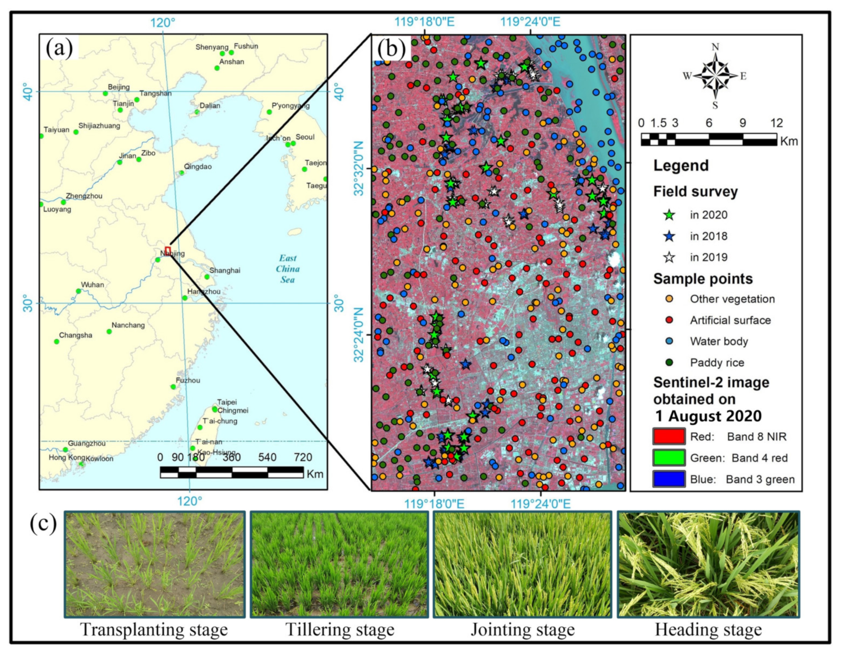
2.1. Study Area

The study area was located in Yangzhou City, Jiangsu Province, China, as shown in Figure 1a,b. It has a subtropical monsoon climate, which is featured with cloudy and rainy weather during the rice growing season. The study area was a representative rice planting area in southern China, where the farmland is small and fragmented and the climate is cloudy and rainy, which makes it an ideal place for testing rice mapping methods. The key growth stages of rice in the study area include the transplanting, tillering, jointing and heading stages, as shown in Figure 1c.

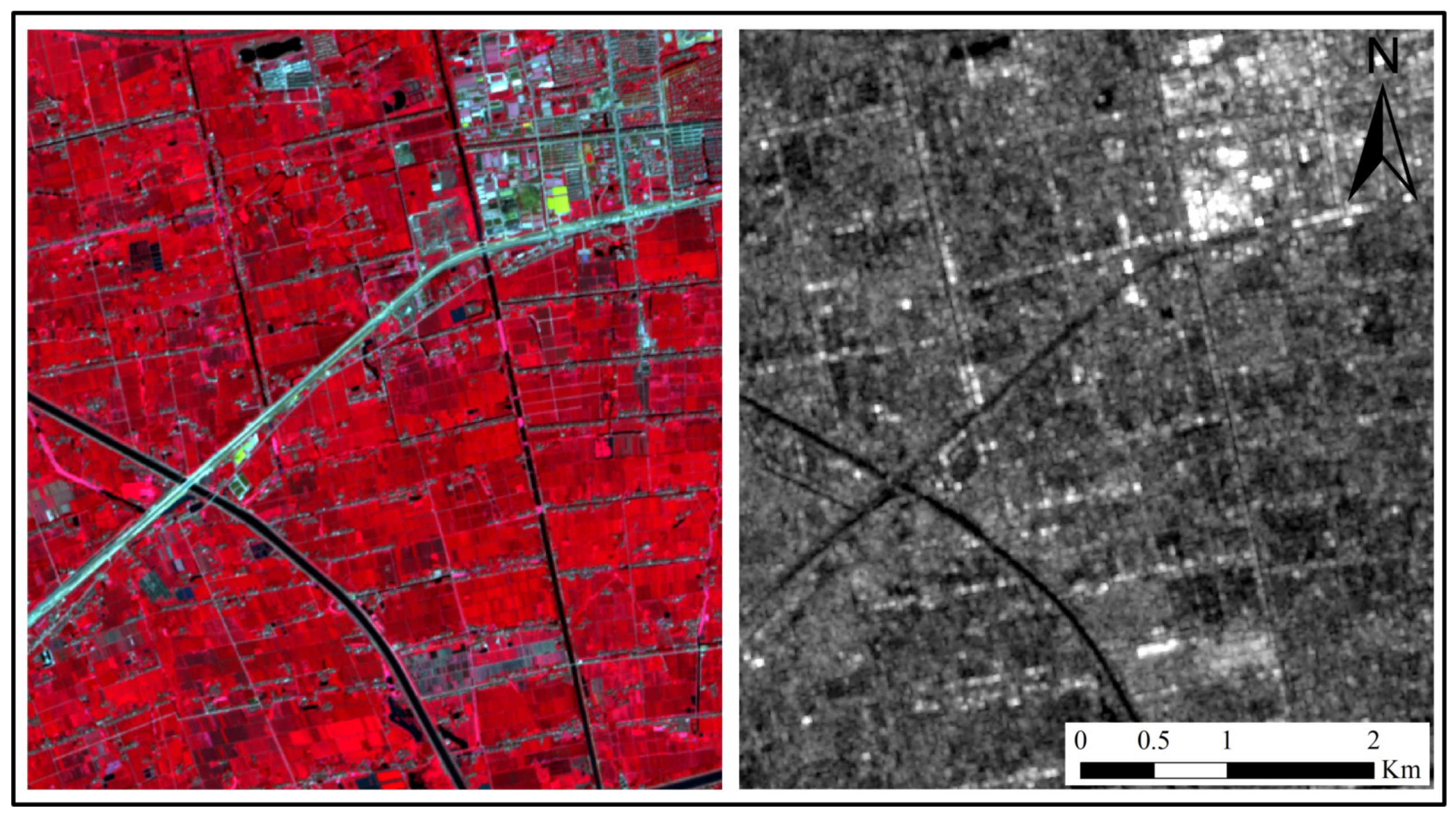
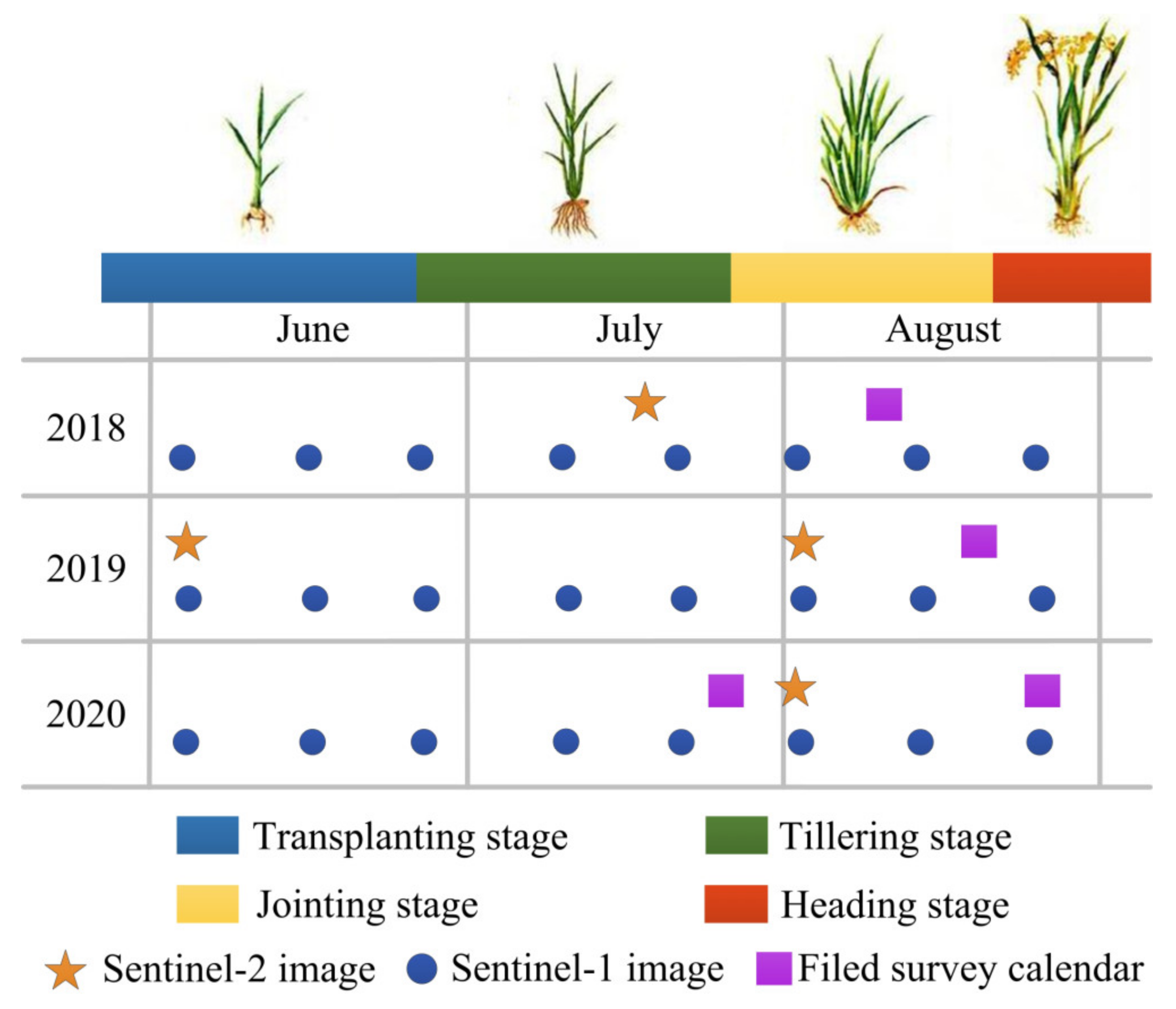
2.2. Remote Sensing and Field Survey Data

Sentinel-1 and Sentinel-2 data acquired between June and August in 2018, 2019 and 2020 were employed in this study (Figure 2). The main parameters of Sentinel-1 and Sentinel-2 images are shown in

Table 1. Main parameters of the used Sentinel-1 and Sentinel-2 images.

Sentinel-1		Sentinel-2
Indicators	Information	Band	Wavelength (μm)	Resolution (m)
Mode	IW	Band1	0.443–0.453	60
Polarization	VV, VH	Band2	0.458–0.523	10
		Band3	0.543–0.578	10
Band	C	Band4	0.650–0.680	10
Resolution	10 m	Band5	0.698–0.713	20
		Band6	0.733–0.748	20
Centre frequency	5.4 GHz	Band7	0.773–0.793	20
		Band8	0.785–0.900	10
Product type	Ground Range Detected (GRDH)	Band9	0.935–0.955	60
		Band10	1.360–1.390	60
Pass direction	Ascending	Band11	1.565–1.655	20
		Band12	2.100–2.280	20

. The acquisition dates of the used satellite images are illustrated in Figure 3. Unlike the SAR data that were continuously acquired from 2018 to 2020, there was only one cloud-free optical image acquired in both 2018 and 2020 (on 18 July which was at the tillering stage in 2018, and on 1 August which was at the jointing stage in 2020, respectively). In 2019, there were only two available cloud-free optical images, which were acquired at the transplanting stage (3 June) and the jointing stage (2 August), respectively.

In addition, field surveys were conducted at the end of the jointing stage on three consecutive years. A total of 96, 151 and 173 rice fields were investigated from 2018 to 2020, respectively. Referring to these field survey samples, 250 rice sample points and 50 regions of interest (ROIs) were further obtained by visual interpretation against a high-resolution image in each year. In this study, by combining sample points with ROIs, the representativeness of the sample can be effectively guaranteed, which is conducive to remote sensing recognition and accuracy verification of ground objects. In addition to rice, the classes corresponding to the water body, artificial surface and other vegetation were also interpreted with 250 sample points and 50 ROIs in each class. Considering the study area’s size and the distribution of ground objects, the samples were trained and validated in a 4:6 ratio (Figure 1). In addition, according to the ground survey and visual interpretation, we drew the boundaries of 80 rice plots to evaluate the performance of multi-scale segmentation.

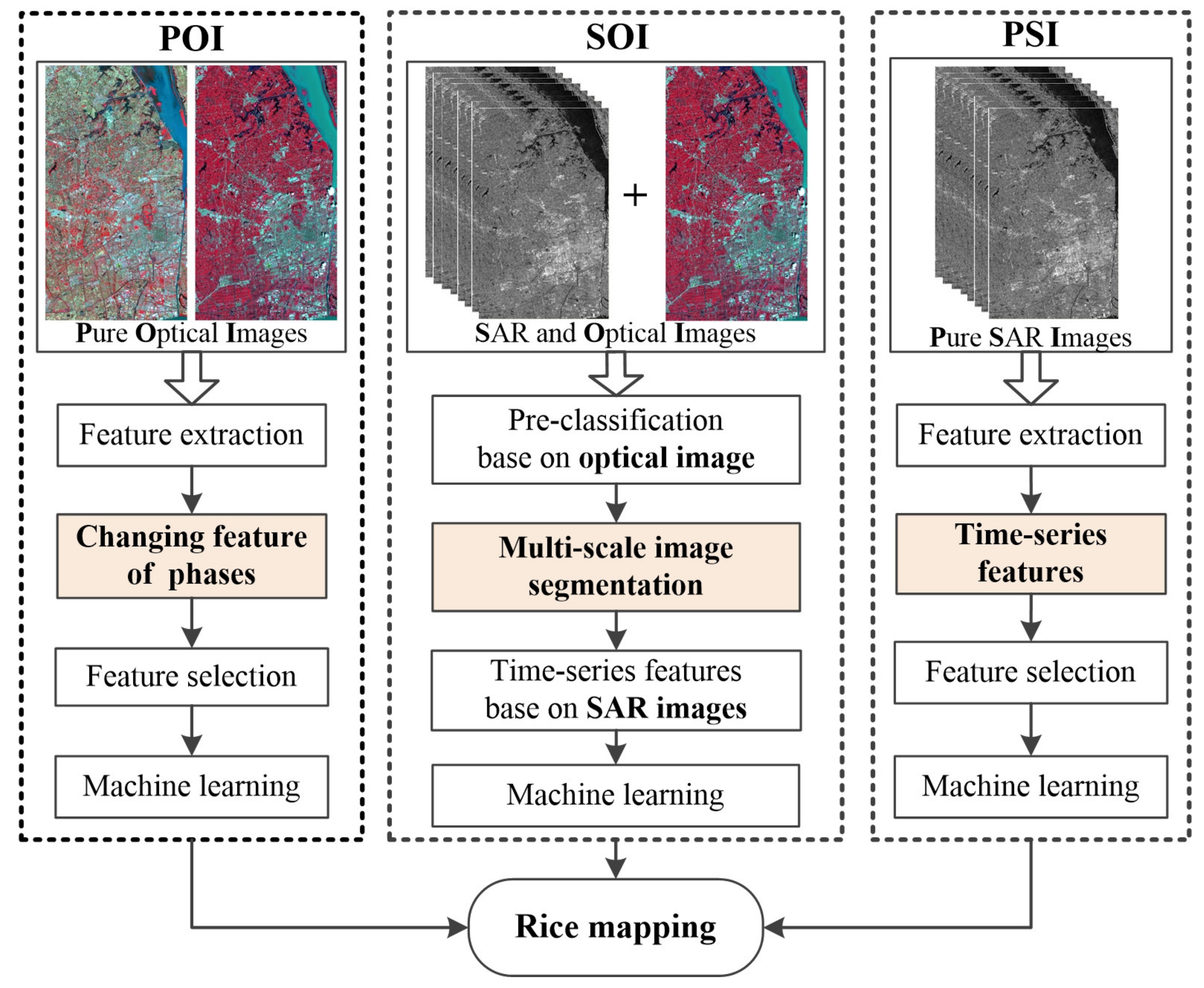
2.3. Methods for Rice Mapping

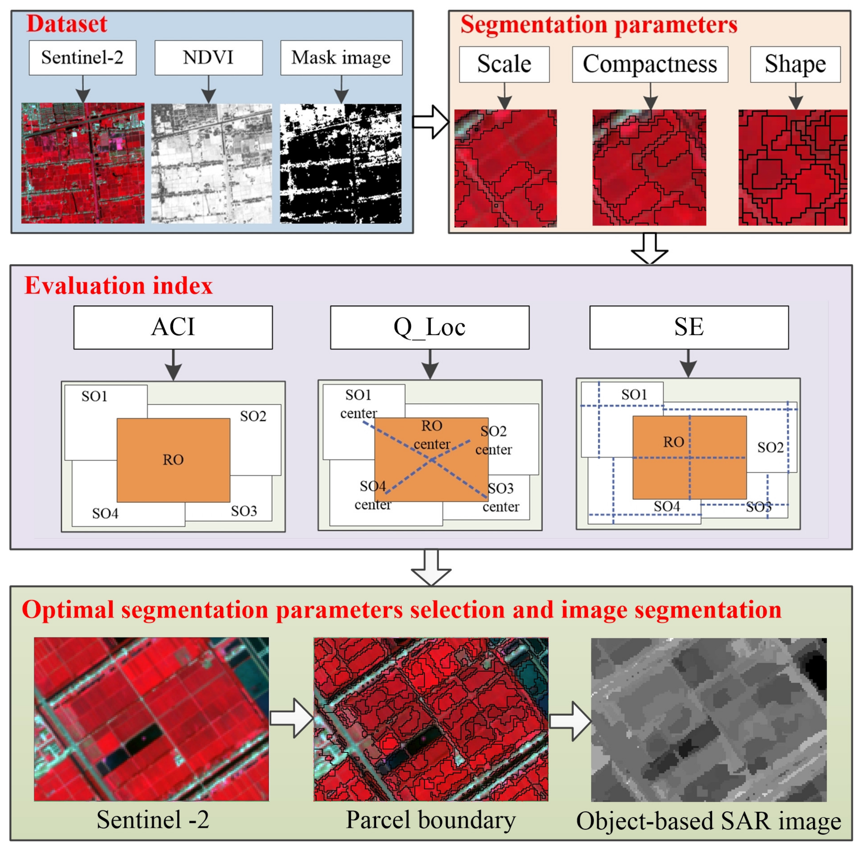
2.3.1. Rice Mapping Method by Fusing SAR and Optical Images (SOI)

Based on the commonly available scenario of “single-phase optical and multi-phase microwave images” in cloudy and rainy regions, this method aims to take full advantage of SAR and optical images in rice mapping, and reduces the dependence on the acquisition time of the optical image. The technical workflow of the method is illustrated in Figure 4, which includes the following steps:

(1)

Preliminary classification based on single-phase optical image

Firstly, with optimized spectral features generated from Sentinel-2 image bands (more details in Section 2.4), a preliminary classification model is established by SVM to exclude some ground objects (i.e., the artificial surface) that are evidently not rice, and thus simplify image segmentation and rice mapping.

(2)

Optical image segmentation and object-based feature extraction from SAR images

A multi-scale segmentation was conducted to extract boundaries of rice parcels based on the Sentinel-2 image and the preliminary classification result. Then, the parcel boundary information is used to handle the features from the SAR time-series images. Detailed processes could be found in Section 2.4 and Section 2.5.

(3)

Rice mapping and evaluation of methods’ adaptability to operational scenario

Based on the object-based time-series SAR features, the classification model for rice mapping is established. In this process, different machine learning algorithms are tested and compared in performance evaluation (details are fully described in Section 2.6). In each of the four rice growth stages, one SAR image is randomly selected to form a time-series of SAR images for rice mapping, so as to test the sensitivity of the proposed method to the slight difference of SAR image acquisition time. Further, to evaluate the capabilities of polarization features and texture features in rice extraction, three different feature sets were compared, including the pure polarization feature set (PPF), the pure texture feature set (PTF), and the joint set of polarization features and texture features (PFTF).

Figure 4. Illustration of the rice mapping method. PPF means the pure polarization feature set; PTF means the pure texture feature set; PFTF means the joint set of polarization features and texture features.

Figure 4. Illustration of the rice mapping method. PPF means the pure polarization feature set; PTF means the pure texture feature set; PFTF means the joint set of polarization features and texture features.

2.3.2. Rice Mapping Methods Based on Pure Optical Images (POI) and Pure SAR Images (PSI) for Comparison

To assess the performance of the SOI method, two conventional strategies that map rice based on pure optical images (POI) and pure SAR images (PSI) were compared. For the POI-based strategy, two Sentinel-2 images on the tillering and jointing stages in 2019 were analyzed. For the PSI-based strategy, the pixel-level classification was conducted based on the time-series microwave images from 2018 to 2020 (Figure 5). For POI and PSI, similar feature selection and machine learning approaches to SOI were adopted.

2.4. Feature Selection for Rice Mapping

Stable and effective features are crucial for rice mapping with remote sensing data. Optimal feature sets were generated from candidate optical and SAR features considering both feature sensitivity and information redundancy for different classification strategies.

(1)

Candidate optical and SAR features

The candidate optical features mainly include 10 spectral band features and 8 classic vegetation indices (VIs) that can effectively indicate the physiological state of plants (

Table 2. Candidate optical and SAR features for rice mapping.

Satellites	Category	Features	Reference
Sentinel-2	Spectral bands	Band2-Blue	/
		Band3-Green
		Band4-Red
		Band5-Vegetation Red Edge
		Band6-Vegetation Red Edge
		Band7-Vegetation Red Edge
		Band8-NIR
		Band9-Water vapor
		Band11-SWIR
		Band12-SWIR
	VIs	EVI = 2.5 × (NIR − Red)/(NIR + 6 × Red − 7.5 × Blue + 1)	[17]
		EVI2 = 2.5 × (NIR − Red)/(NIR + 2.4 × Red + 1)	[18]
		SR = NIR/R	[19]
		NDVI = (NIR − Red)/(NIR + Red)	[20]
		SAVI = (NIR − Red) × (1 + L)/(NIR + Red + L)	[21]
		WDRVI = (0.1 × NIR − Red)/(0.1 × NIR + Red)	[22]
		MNDWI = (Green − SWIR)/(Green + SWIR)	[23]
		VARIred-edge = (Red-edge − Red)/(Red-edge + Red)	[24]
Sentinel-1	Polarization	VV	/
		VH
	Textural features	Mean	[16]
		Variance
		Homogeneity
		Contrast
		Dissimilarity
		Entropy
		Second Moment
		Correlation

). These VIs are sensitive to vegetation targets and are frequently used for crop mapping and monitoring [15]. The candidate SAR features mainly include 2 polarization features and 8 texture features that are generated by the gray-scale co-occurrence matrix (with a 5×5 window and 32 levels). The VV and VH polarization are significantly affected by variation of soil moisture and canopy structure. The texture features of SAR images are derived from the gray co-occurrence matrix that are able to provide information about the spatial pattern among image pixels (Table 2) [16]. The above features were extracted by ENVI 5.3 software.

(2)

Selection of features for preliminary classification

Among the 18 candidate optical features in Table 2, an independent t-test was used to evaluate their sensitivity in classifying the four ground object types, with a criteria of p < 0.01. Within the sensitive features, a correlation analysis was carried out among features to reduce information redundancy. The R² > 0.8 was used as the relevant criterion for each pair of features. Combined with the sensitivity result of the t-test, the features with weak sensitivity were eliminated according to the p-value until no features were highly correlated. As a result, this yielded the optimized feature set with strong sensitivity and low correlation for preliminary classification.

(3)

Selection of temporal change optical features

To use the temporal change information of optical features on two growth stages of rice, the difference of the candidate features (Table 2) was derived between the transplanting stage and the jointing stage (Formula (1)).

$$F_{\Delta }=F_{p2}-F_{p1}$$

(1)

where F represents a certain feature, F_p1 and F_p2 represent the feature on transplanting stage and jointing stage, and F_∆ represents the change of this feature.

Based on the temporal change features, the same approach for conducting sensitivity analysis and cross-correlation analysis were implemented to generate the optimized temporal change feature set. These features, together with optimal features for preliminary classification, were used for rice mapping under POI mode.

(4)

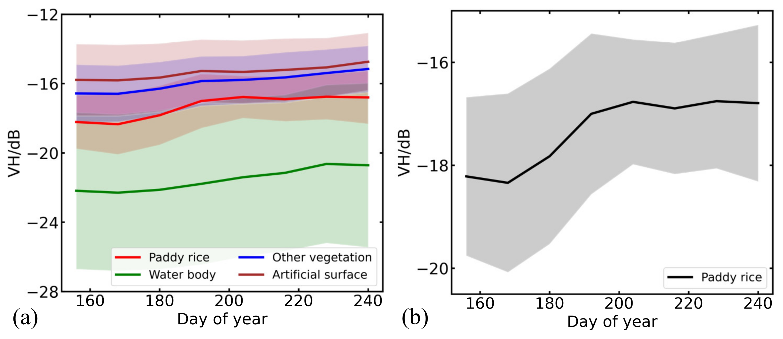
Selection of SAR features

The polarization and texture features on each SAR image were averaged according to the generated ROIs (details please see Section 2.5). Based on these extracted data, the same feature elimination process as used in previous steps was implemented to obtain the optimized SAR features.

2.5. Multi-Scale Image Segmentation

Multi-scale segmentation is used to segment the image into parcel objects. In multi-scale segmentation, the selection of segmentation parameters directly associates with the consistency between the derived boundaries and actual boundaries of natural plots [25], which significantly affects the accuracy of rice mapping. To assess the results of the segmentation, a set of objective and quantifiable evaluation indices are needed.

In this study, a representative region was selected in the study area for determining the segmentation parameters. The optimized parameters were then applied to the whole study area. As the Figure 6 shows, in the multi-scale image segmentation analysis, the original bands (Band3 to Band8) and NDVI feature of the Sentinel-2 image were used as the base images. According to both the literature and pre-experiment results [26,27], the range and step of the segmentation parameters are determined as scale factor: 35–60 with a step of 5; shape factor: 0.1–0.6 with a step of 0.1; and compactness factor: 0.2–0.7 with a step of 0.1. A three-factor and six-level orthogonal experiment [28] was conducted to avoid traversal testing, yielded a total of 36 factor combinations for optimizing parameters.

Regarding the quality evaluation of the multi-scale segmentation, three indices, including the area consistency index (ACI), shape error (SE) and quality of an individual object’s location (Q_Loc), were used to provide a comprehensive evaluation. The principle of the three indices is illustrated in Figure 6, and their formulas are given as follows:

$$AC{I}_i=\frac{area\left(S{O}_i\cap R{O}_i\right)}{area\left(S{O}_i\cup R{O}_i\right)}$$

(2)

$$Q\_Lo{c}_i=dist\left(centroid\left(S{O}_i\right),centroid\left(R{O}_i\right)\right)$$

(3)

$$S{E}_i=\left|Asr\left(S{O}_i\right)-Asr\left(R{O}_i\right)\right|$$

(4)

where the ACI refers to the ratio of the overlap between the segmented object (SO) and the reference object (RO) to their merged area. When the SO is close to RO, the ACI approaches 1, indicating the ideal result. The Q_Loc represents the sum of the distances between the centroids of RO and SO. The SE calculates the aspect ratio between the SO and the RO [29,30], and Asr represents the aspect ratio.

Based on the three indices, a comprehensive segmentation score (CSS, Formula (5)) is proposed, which is the sum of the sequential score of each index (e.g., for one index, the highest score, 36, indicates the combination ranking no. 1). The combination corresponding to the highest CSS is determined as the optimal parameter set and was used to conduct the multi-scale segmentation.

$$CSS=\mathrm{Sequential} \mathrm{Score}\left(ACI+Q\_Loc+SE\right)$$

(5)

2.6. Classification Method and Evaluation

Based on the optimized features extracted from the segmented blocks, two representative machine learning algorithms, the CART and SVM, were used for rice mapping. The CART is a classic method for adaptively constructing a decision tree classifier according to the relationships among variables. The algorithm is easy to be interpreted, superior in processing a large amount of high-dimensional data and solving nonlinear problems [4]. The SVM seeks the optimal hyperplane for different categories of samples by projecting the variables into a high-dimensional feature space, which has good generalization ability and advances, particularly for small-size samples [9,31].

The evaluation of rice mapping results, including the overall accuracy (OA), user’s accuracy (UA), producer’s accuracy (PA) and kappa coefficient, are all calculated from the confusion matrix [9]. In this study, the eCognition software was used for multi-scale image segmentation, the ENVI software was used for image processing, and the Matlab software was used for data analysis.

3. Results

3.1. Optimal Features for Rice Mapping

The sensitivity of optical features for preliminary classification are shown in

Table 3. Results of sensitivity analysis with the single-scene Sentinel-2 image.

Category	Features	t-Test	Cross-Correlation
Spectral bands	Band2
	Band3
	Band4	▲	■
	Band5
	Band6	▲
	Band7	▲
	Band8	▲
	Band9	▲
	Band11	▲	■
	Band12	▲
VIs	EVI	▲	■
	EVI2	▲
	SR
	NDVI
	SAVI	▲	■
	WDRVI
	MNDWI	▲	■
	VARIred-edge	▲

“▲” indicates that the t-test results of the specific feature achieved p < 0.01 significance level, and “■” indicates the final features selected under correlation analysis R² < 0.8.

. All bands except Band2, Band3 and Band5 achieved the significance level of p < 0.01. The EVI, EVI2, SAVI, MNDWI and VARI_red-edge all exceeded the significance level of 0.01. However, a high cross-correlation was found between these features. After removing those features with redundant information, only Band4, Band11, EVI, MNDWI and SAVI were retained.

Meanwhile, according to same feature selection steps above, the optimal features for POI-based classification are Band3_∆, Band6_∆, Band9_∆, EVI_∆ and WDRVI_∆.

Based on segmented parcel boundaries, the SAR features are extracted and processed with sensitivity analysis. It was noticed that the VH value of the water body is significantly lower than that of the other classes, while rice has a lower backscattering coefficient compared with other classes, except water (Figure 7). The VH backscattering coefficient of rice is low in the transplanting stage, and gradually increases with the growth of the plants, which exhibited a clear temporal pattern. According to the similar t-test and cross-correlation check, the sensitivity of the SAR features was derived and illustrated in

Table 4. Sensitivity of SAR features on different dates.

Features	Date (2018)
	Phase1 (0603)	Phase2 (0615)	Phase3 (0627)	Phase4 (0709)	Phase5 (0721)	Phase6 (0802)	Phase7 (0814)	Phase8 (0826)
VV				▲	▲			▲
VV_Mean	▲		▲			▲
VV_Variance				▲	▲
VV_Homogeneity
VV_Contrast
VV_Dissimilarity				▲	▲
VV_Entropy				▲	▲
VV_Second Moment
VV_Correlation
VH		▲					▲
VH_Mean	▲
VH_Variance					▲	▲
VH_Homogeneity		▲			▲	▲
VH_Contrast						▲
VH_Dissimilarity					▲	▲	▲
VH_Entropy			▲			▲
VH_Second Moment		▲						▲
VH_Correlation						▲		▲

The dates in the table are from 2018. In 2019 and 2020, the acquisition dates are one day postponed compared to 2018. “▲” indicates that the t-test results of the specific feature achieved the p < 0.01 significance level, and the final features were selected under correlation analysis R² < 0.8.

. There are more sensitive features identified on the tillering stage (9 July and 21 July) and jointing stage (2 August). More VH polarization features are found to be sensitive than the VV polarization features. For texture features, the dissimilarity, mean, variance and entropy features are sensitive to rice mapping. However, the texture features are generally not as sensitive as polarization features.

To further test the adaptability of the proposed method, the 30 optimized features were grouped according to four key growth stages of rice, and combined according to PPF, PTF and PFTF. On each growth stage, only one feature was randomly selected to test the influence of the slight difference in image acquisition time on classification results (

Table 5. A summary of selected SAR features on key growth stages of rice.

Combinations	Randomly Selected Features
PPF	VH_Phase2, VV_Phase5, VH_Phase7, VV_Phase8
PTF	VV_Mean_Phase1, VV_Dissimilarity_Phase4, VH_Entropy_Phase6, VV_Second Moment_Phase8,
PFTF	VH_Homogeneity_Phase2, VV_Phase5, VH_Variance_Phase6, VV_Phase8

).

3.2. Rice Parcel Boundaries Yielded by Multi-Scale Segmentation

The orthogonal experiment method was conducted, and the CSS index was calculated for each combination of segmentation parameters. The combination corresponding to the highest CSS is determined as the optimal combination. In this case, the segmentation parameters are: scale = 35, shape = 0.3, compactness = 0.6. The scale parameter controls the size of the generated object and has a decisive influence on classification accuracy. When the scale is small (e.g., 15), the results tend to be over-segmented, while when the scale is large (e.g., 60), the under-segmented issue tends to be significant. In case the scale is 35, the segmented blocks are approximately similar to the actual rice parcels (Figure 8).

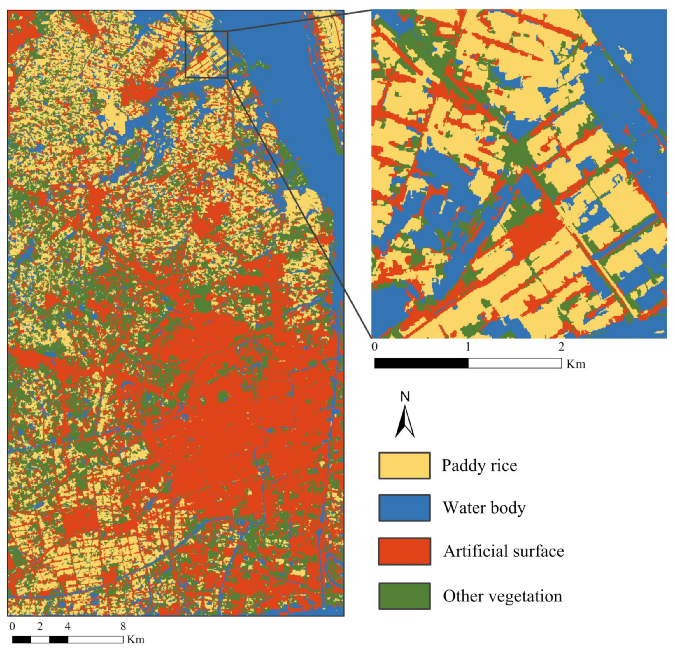
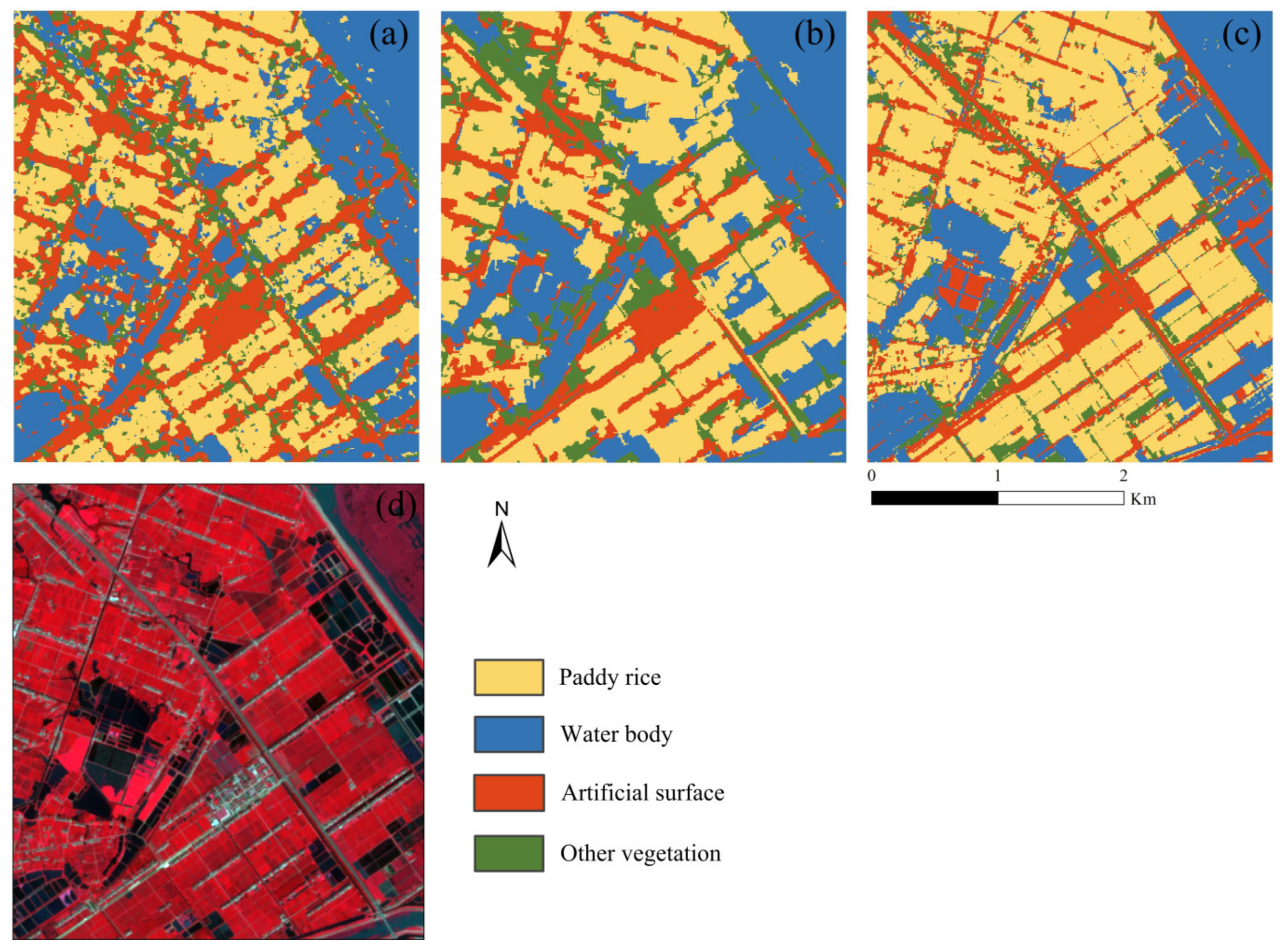
3.3. Evaluation of Rice Mapping Results

Rice planting area mapped with different strategies (i.e., SOI, POI and PSI, for details please see Section 2.3) in 2018–2020 are shown in Figure 9 and Figure 10. Figure 9 shows that rice is mainly distributed in the northern part of the study area, while the southern part of the study area is dominated by artificial surfaces. Figure 10 shows that the rice classification results obtained by the POI method are the least fragmented, but there are some misclassifications (e.g., the pond is misclassified as rice), and the rice classification results obtained by the PSI method show an obvious salt and pepper effect, which is mainly caused by the significant noise of the SAR images. The SOI method gives better consideration to the accuracy of classification results, together with the integrity of classified rice parcels. The OA of rice mapping exceeded 90% for both the CART and SVM classifiers under SOI. A remarkably high overall accuracy (93.95%) was achieved for the SVM model, with the PA average and UA average reaching 92.83% and 90.48% (

Table 6. The accuracy of rice mapping results under the SOI strategy. CART means classification and regression trees method; SVM means support vector machine method. OA means overall accuracy; UA means user’s accuracy and PA means producer’s accuracy.

Classifier	Date	OA (%)	OA Average	Kappa	Rice
					PA (%)	PA Average	UA (%)	UA Average
CART	2018	90.61	91.85	0.85	87.22	85.37	88.40	87.88
	2019	94.04		0.91	84.05		87.23
	2020	90.89		0.87	84.85		88.01
SVM	2018	92.42	93.95	0.88	91.33	92.83	95.03	90.48
	2019	94.64		0.92	92.18		84.03
	2020	94.80		0.92	94.97		92.37

), which were slightly higher than those of CART.

The accuracies of SOI were significantly higher than those of PSI. For example, based on SVM, the OA, PA, UA and Kappa of the PSI strategy were lower than the SOI strategy by 9.75%, 19.4%, 18.74% and 0.16, respectively (

Table 7. Accuracy of rice mapping under different strategies.

Classifier	Strategy	OA (%)	Kappa	Rice
				PA (%)	UA (%)
CART	POI	94.02	0.91	96.66	76.05
	SOI	94.04	0.91	84.05	87.23
	PSI	82.35	0.72	71.64	65.62
SVM	POI	97.83	0.97	97.71	95.61
	SOI	94.64	0.92	92.18	84.03
	PSI	84.89	0.76	72.78	65.29

The results are based on the 2019 dataset.

). This suggests that the addition of the parcel boundary information plays a vital role in rice mapping. Conversely, for SOI and POI, the results indicated that under the commonly available scenario of “single-phase optical and multi-phase microwave images”, the SOI can yield approximate accuracy to the POI strategy in rice mapping. In addition, the performance of the POI is somewhat unstable. The UA of the CART model is only 76.05%, indicating significant misclassification from the water body to rice (Table 7 and

Table 8. Confusion matrix of the CART model under POI strategy.

		Truth
		Paddy Rice	Water Body	Artificial Surface	Other Vegetation	Total
Classification	Paddy rice	927	215	12	65	1219
	Water body	17	3598	8	46	3669
	Artificial surface	14	2	1680	31	1727
	Other vegetation	1	5	17	607	630
	Total	959	3820	1717	749	7245

The results are based on data from 2019.

).

To further assess the adaptability of SOI in the operational scenario, three randomly picked SAR image sets were used to substitute the entire SAR image time series. The results of SVM models showed that PPF achieved relatively high accuracies, whereas the accuracies of PTF were lower (

Table 9. Accuracy of rice mapping with randomly picked SAR images.

Combinations	Date	OA (%)	OA Average	Kappa	Rice
					PA (%)	PA Average	UA (%)	UA Average
PPF	2018	88.12	90.09	0.81	79.69	85.10	85.70	87.43
	2019	92.74		0.89	90.93		86.94
	2020	89.41		0.84	84.67		89.66
PTF	2018	84.57	85.58	0.76	76.02	72.71	58.98	60.20
	2019	86.63		0.79	70.80		58.08
	2020	85.55		0.79	71.32		63.55
PFTF	2018	89.62	88.81	0.84	87.12	85.60	91.63	90.02
	2019	86.03		0.78	84.88		92.71
	2020	90.79		0.86	84.79		85.71

). Such a pattern indicates that polarization features are more effective in rice mapping than texture features.

In comparing the operational PFTF model (Table 9) with the model with the entire SAR time series (Table 6), despite the accuracy of the PFTF model being slightly lower than that of the model with the entire SAR time series, the accuracy of rice mapping is still acceptable. This suggests that the SOI can also be driven by only SAR images on several key growth stages of rice, which thus illustrates a great potential in the operational implementation of rice mapping.

4. Discussion

4.1. Role of Optical and SAR Features for Rice Mapping

Throughout the growing progress of rice, it shows significant changes in optical and SAR features, which help to distinguish it from other land objects. For example, the significant increase of the rice leaf area during the tillering stage and jointing stage will induce the response of several Vis [15,21]. For SAR images, the backscattering intensity is governed by the composition of the soil and the structure of the rice canopy. In the transplanting stage of rice, the microwave signal was dominated by mirror reflection of the water surface, which is similar to the response of the water body. During the tillering to ridge sealing stages of rice, the body scattering and canopy scattering increased, and lead to an increase of the backscattering coefficient. Conversely, during the ridge sealing to heading stages, the canopy coverage of rice is stable, and the canopy scattering played a dominant role, thus leading to a slight decrease of the backscattering coefficient. The variation of canopy composition and canopy structure of rice across the growth stages thus forms the theoretical basis of rice mapping with SAR features [4,11].

The polarization features of the SAR image can reflect the degree of interaction between vegetation structures, while the textural features of the SAR image can delineate the spatial relationship and structure distribution of ground objects [16]. The complementary characteristics between these two types of features help to improve the efficacy of rice recognition.

4.2. Optimization of Multi-Scale Segmentation

Different from some existing studies that evaluate multi-scale segmentation results using a single criterion (e.g., common area ratio; distance between objects’ centers, etc.) [32], this study combines a set of evaluation indices and an orthogonal experiment to provide a comprehensive optimization of segmentation parameters. The evaluation method considers the area consistency, shape error and location of objects, which ensures the high quality of segmented parcels’ boundaries.

It should also be noticed that although the ideal block boundaries can be obtained for most parcel fields under optimal segmentation parameters, some non-ideal segments also existed in results. Within a certain region, the heterogeneity of the landscape resulted in difference in the category, size and spectral characteristics of the ground object. This may be because the landscape heterogeneity (i.e., size, spectral characteristics, etc.) makes it difficult to achieve satisfactory segmentation for all parcels using one set of segmentation parameters for a large area [33]. Therefore, it might be necessary to adjust these segmentation parameters in different parts for a large area to improve the quality of the segmentation.

4.3. The Effectiveness of the SOI

The SOI strategy fully considers the climatic characteristic of cloudy and rainy regions where the acquisition time of optical images is uncertain. The role of the optical images is changed from classification to field segmentation, which thus loosen the requirement of the acquisition time of optical images. Therefore, within 2018–2020, despite the optical images being acquired at different rice growth stages, a relatively stable accuracy can be achieved in rice mapping, which guarantees the robustness of the strategy. Yang et al. [11] combined multi-scene optical images with time-series microwave images for rice mapping, and the classification accuracy reached 90.2%. In contrast, the SOI method proposed in this paper achieved a higher rice mapping accuracy (94.64%), while reducing the dependency on multi-temporal optical images. On the other hand, the SAR images can capture the specific temporal change pattern of rice. However, the inherent salt and pepper issue of the SAR images severely disturbs the temporal pattern of the SAR, which further limits the accuracy of rice mapping based on pixel-level SAR images [34,35]. However, by averaging the SAR image features according to the segmented parcels, the noise issue can be effectively suppressed in object-oriented rice mapping and obtain a higher accuracy.

Further, it is encouraging that the SOI strategy can be driven solely by a few SAR images from four key growth stages of rice, yet still achieve satisfactory classification accuracy. It is anticipated that the SAR features from the four key growth stages of rice reflect the major temporal change pattern during the rice development process. With significantly less input data, the computational complexity of the procedure can be reduced, which is important in an operational scenario. In addition, considering that long-term time-series SAR data can effectively improve the differences between different ground objects, especially different vegetation, and thus improve the classification accuracy, this study does not discuss the situation when all SAR data are in the same phenological stage.

5. Conclusions

In this study, aiming at rice mapping that can be operationally implemented in cloudy and rainy regions, a strategy by fusing SAR and optical images is proposed. The main conclusions are as follows:

(1)

The proposed SOI method can achieve accurate extraction of rice area. The method makes full use of the parcel boundary information derived by optical images and growth and phonological traits of rice from SAR images. The mapping accuracy of SOI is significantly higher than PSI and POI.

(2)

An adaptive rice parcel boundary extraction method based on multi-scale segmentation was proposed. A comprehensive segmentation quality index, together with an orthogonal experiment, were used to obtain the optimal segmentation parameters and generate the parcel boundaries for rice mapping.

(3)

Further, the adaptability of SOI in the operational scenario is examined according to a “random pick” strategy. Based on both the polarization and texture features, the SOI method exhibited strong adaptability to the uncertainty of the acquisition time of remote sensing images.

It should be noted that some challenges remain in the application of the established method. For example, some regions may have different cultivation schemes (e.g., different timing of transplanting, different plans of irrigating) and different growth period durations, which may result in the inconsistency of temporal signals and thus hamper the implementation of the proposed SOI strategy. In addition, in areas with high spatial heterogeneity, the issue of mixed pixels may also interfere with the rice mapping results. However, it is encouraging that abundant remote sensing data with constantly improving spatial and temporal resolution provide a powerful backing of remotely sensed rice mapping. In addition, the achievement of deep learning algorithms can also be considered in the future, particularly in some more complicated scenarios in rice mapping.

References

1. Godfray, H.C.J.; Beddington, J.R.; Crute, I.R.; Haddad, L.; Lawrence, D.; Muir, J.F.; Pretty, J.; Robinson, S.; Thomas, S.M.; Toulmin, C. Food security: The challenge of feeding 9 billion people. Science 2010, 327, 812–818. [Google Scholar] [CrossRef] [PubMed] [Green Version]
2. Lobell, D.B.; Thau, D.; Seifert, C.; Engle, E.; Little, B. A scalable satellite-based crop yield mapper. Remote Sens. Environ. 2015, 164, 324–333. [Google Scholar] [CrossRef]
3. Peng, D.L.; Huete, A.R.; Huang, J.F.; Wang, F.M.; Sun, H.S. Detection and estimation of mixed paddy rice cropping patterns with MODIS data. Int. J. Appl. Earth Obs. Geoinf. 2011, 13, 13–23. [Google Scholar] [CrossRef]
4. Talema, T.; Hailu, B.T. Mapping rice crop using sentinels (1 SAR and 2 MSI) images in tropical area: A case study in Fogera wereda, Ethiopia. Remote Sens. Appl. Soc. Environ. 2020, 18, 100290. [Google Scholar] [CrossRef]
5. Ali, A.M.; Savin, I.; Poddubsky, A.; Abouelghar, M.; Saleh, N.; Abutaleb, K.; El-Shirbeny, M.; Dokuin, P. Integrated Method for Rice Cultivation Monitoring Using Sentinel-2 Data and Leaf Area Index. Egypt. J. Remote Sens. Space Sci. 2020, 24, 431–441. [Google Scholar] [CrossRef]
6. Dong, J.W.; Xiao, X.M.; Menarguez, M.A.; Zhang, G.L.; Qin, Y.W.; Thau, D.; Biradar, C.; Moore, B., III. Mapping paddy rice planting area in northeastern Asia with Landsat 8 images, phenology-based algorithm and Google Earth Engine. Remote Sens. Environ. 2016, 185, 142–154. [Google Scholar] [CrossRef] [Green Version]
7. Phung, H.P.; Nguyen, L.D.; Thong, N.H.; Thuy, L.T.; Apan, A.A. Monitoring rice growth status in the Mekong Delta, Vietnam using multitemporal Sentinel-1 data. J. Appl. Remote Sens. 2020, 14, 1. [Google Scholar] [CrossRef] [Green Version]
8. Zhan, P.; Zhu, W.Q.; Li, N. An automated rice mapping method based on flooding signals in synthetic aperture radar time series. Remote Sens. Environ. 2021, 252, 112112. [Google Scholar] [CrossRef]
9. Mansaray, L.R.; Wang, F.M.; Huang, J.F.; Yang, L.B.; Kanu, A.S. Accuracies of support vector machine and random forest in rice mapping with Sentinel-1A, Landsat-8 and Sentinel-2A datasets. Geocarto Int. 2020, 35, 1088–1108. [Google Scholar] [CrossRef]
10. Xiao, W.; Xu, S.C.; He, T.T. Mapping Paddy Rice with Sentinel-1/2 and Phenology-, Object-Based Algorithm-A Implementation in Hangjiahu Plain in China Using GEE Platform. Remote Sens. 2021, 13, 990. [Google Scholar] [CrossRef]
11. Yang, H.J.; Pan, B.; Wu, W.F.; Tai, J.H. Field-based rice classification in Wuhua county through integration of multi-temporal Sentinel-1A and Landsat-8 OLI data. Int. J. Appl. Earth Obs. Geoinf. 2018, 69, 226–236. [Google Scholar] [CrossRef]
12. He, Y.L.; Dong, J.W.; Liao, X.Y.; Sun, L.; Wang, Z.P.; You, N.S.; Li, Z.C.; Fu, P. Examining rice distribution and cropping intensity in a mixed single-and double-cropping region in South China using all available Sentinel 1/2 images. Int. J. Appl. Earth Obs. Geoinf. 2021, 101, 102351. [Google Scholar] [CrossRef]
13. Yang, L.B.; Wang, L.M.; Abubakar, G.A.; Huang, J.F. High-Resolution Rice Mapping Based on SNIC Segmentation and Multi-Source Remote Sensing Images. Remote Sens. 2021, 13, 1148. [Google Scholar] [CrossRef]
14. Yang, L.B.; Mansaray, L.R.; Huang, J.F.; Wang, L.M. Optimal Segmentation Scale Parameter, Feature Subset and Classification Algorithm for Geographic Object-Based Crop Recognition Using Multisource Satellite Imagery. Remote Sens. 2019, 11, 514. [Google Scholar] [CrossRef] [Green Version]
15. Thenkabail, P.S.; Lyon, J.G.; Huete, A. Hyperspectral Remote Sensing of Vegetation; CRC Press: Boca Raton, FL, USA, 2011; pp. 336–348. [Google Scholar]
16. Caballero, G.R.; Platzeck, G.; Pezzola, A.; Casella, A.; Winschel, C.; Silva, S.S.; Luduena, E.; Pasqualotto, N.; Delegido, J. Assessment of Multi-Date Sentinel-1 Polarizations and GLCM Texture Features Capacity for Onion and Sunflower Classification in an Irrigated Valley: An Object Level Approach. Agron. J. 2020, 10, 845. [Google Scholar] [CrossRef]
17. Huete, A.; Didan, K.; Miura, T.; Rodriguez, E.P.; Gao, X.; Ferreira, L.G. Overview of the radiometric and biophysical performance of the MODIS vegetation indices. Remote Sens. Environ. 2002, 83, 195–213. [Google Scholar] [CrossRef]
18. Jiang, Z.Y.; Huete, A.R.; Didan, K.; Miura, T. Development of a two-band enhanced vegetation index without a blue band. Remote Sens. Environ. 2008, 112, 3833–3845. [Google Scholar] [CrossRef]
19. Jordan, C.F. Derivation of Leaf-Area Index from Quality of Light on the Forest Floor. Ecology 1969, 50, 663–666. [Google Scholar] [CrossRef]
20. Rouse, J.W.; Haas, R.H.; Schell, J.A.; Deering, D.W. Monitoring vegetation systems in the great plains with ERTS. Nasa Spec. Publ. 1974, 351, 309. [Google Scholar]
21. Huete, A.R. A soil-adjusted vegetation index (SAVI). Remote Sens. Environ. 1988, 25, 295–309. [Google Scholar] [CrossRef]
22. Gitelson, A.A. Wide Dynamic Range Vegetation Index for Remote Quantification of Biophysical Characteristics of Vegetation. J. Plant Physiol. 2004, 161, 165–173. [Google Scholar] [CrossRef] [PubMed]
23. Xu, H.Q. A Study on Information Extraction of Water Body with the Modified Normalized Difference Water Index (MNDWI). J. Remote Sens. 2005, 9, 7, (In Chinese with English Abstract). [Google Scholar]
24. Gitelson, A.A.; Kaufman, Y.J.; Stark, R.; Rundquist, D. Novel algorithms for remote estimation of vegetation fraction. Remote Sens. Environ. 2002, 80, 76–87. [Google Scholar] [CrossRef] [Green Version]
25. Mesner, N.; Ostir, K. Investigating the impact of spatial and spectral resolution of satellite images on segmentation quality. J. Appl. Remote Sens. 2014, 8, 083696. [Google Scholar] [CrossRef]
26. Bo, S.K.; Han, X.C.; Ding, L. Automatic Selection of Segmentation Parameters for Object Oriented Image Classification. Geomat. Inf. Sci. Wuhan Univ. 2009, 34, 514–517, (In Chinese with English Abstract). [Google Scholar]
27. Zhu, C.J.; Yang, S.Z.; Cui, S.C. Accuracy evaluating method for object-based segmentation of high resolution remote sensing image. High Power Laser Part. Beams 2015, 27, 27061007, (In Chinese with English Abstract). [Google Scholar]
28. Sui, D.S.; Cui, Z.S. Application of orthogonal experimental design and Tikhonov regularization method for the identification of parameters in the casting solidification process. Acta Metall. Sin. 2009, 22, 9. [Google Scholar] [CrossRef] [Green Version]
29. Zhan, Q.M.; Molenaar, M.; Tempfli, K.; Shi, W.Z. Quality assessment for geo-spatial objects derived from remotely sensed data. Int. J. Remote Sens 2005, 26, 2953–2974. [Google Scholar] [CrossRef]
30. Clinton, N.; Holt, A.; Scarborough, J.; Yan, L.; Gong, P. Accuracy assessment measures for object-based image segmentation goodness. Photogramm. Eng. Remote. Sens 2008, 76, 289–299. [Google Scholar] [CrossRef]
31. Zhang, J.C.; He, Y.H.; Yuan, L.; Liu, P.; Zhou, X.F.; Huang, Y.B. Machine Learning-Based Spectral Library for Crop Classification and Status Monitoring. Agronomy 2019, 9, 496. [Google Scholar] [CrossRef] [Green Version]
32. Rasanen, A.; Rusanen, A.; Kuitunen, M.; Lensu, A. What makes segmentation good? A case study in boreal forest habitat mapping. Int. J. Remote Sens 2013, 34, 8603–8627. [Google Scholar] [CrossRef]
33. Costa, H.; Foody, G.M.; Boyd, D.S. Supervised methods of image segmentation accuracy assessment in land cover mapping. Remote Sens. Environ. 2018, 205, 338–351. [Google Scholar] [CrossRef] [Green Version]
34. Mansaray, L.R.; Zhang, D.; Zhou, Z.; Huang, J. Evaluating the potential of temporal Sentinel-1A data for paddy rice discrimination at local scales. Remote Sens. Lett. 2017, 8, 967–976. [Google Scholar] [CrossRef]
35. Mandal, D.; Kumar, V.; Bhattacharya, A.; Rao, Y.S.; Siqueira, P.; Bera, S. Sen4Rice: A processing chain for differentiating early and late transplanted rice using time-series Sentinel-1 SAR data with Google Earth engine. IEEE Geosci. Remote Sens. Lett. 2018, 15, 1947–1951. [Google Scholar] [CrossRef]
Figure 1. Geographical location of the study area, field survey and sample points. (a) Location of the study area; (b) field survey and sample points in the study area; (c) four key growth stages of rice in the study area.
Agronomy 12 03010 g001
Figure 2. A demonstration of optical (Sentinel-2, Red: Band8, Green: Band4, Blue: Band3) and synthetic aperture radar (SAR) (Sentinel-1 VV) images.
Agronomy 12 03010 g002
Figure 3. Field survey calendar and available remote sensing images within 2018–2020.
Agronomy 12 03010 g003
Figure 5. A comparison of different strategies for rice mapping.
Agronomy 12 03010 g005
Figure 6. Overview of the multi-scale image segmentation for parcel boundary extraction.
Agronomy 12 03010 g006
Figure 7. Temporal curves of SAR features in 2019. (a) Temporal curves of four classes; (b) temporal curve of rice. The light buffers refer to ±1σ from the mean.
Agronomy 12 03010 g007
Figure 8. A demonstration of multi-scale segmentation results under different scale parameters. Shape and compactness are defined as 0.3 and 0.6 here.
Agronomy 12 03010 g008
Figure 9. Rice mapping result based on the SOI strategy in 2019.
Agronomy 12 03010 g009
Figure 10. Comparison of rice mapping results using different classification strategies based on SVM and the 2019 dataset: (ac) represent the partial result under PSI, SOI and POI; (d) represents the false color image of Sentinel-2 (Red: Band8, Green: Band4, Blue: Band3).
Agronomy 12 03010 g010