A Model for Identifying Soybean Growth Periods Based on Multi-Source Sensors and Improved Convolutional Neural Network

Abstract

The identification of soybean growth periods is the key to timely take field management measures, which plays an important role in improving yield. In order to realize the discrimination of soybean growth periods under complex environments in the field quickly and accurately, a model for identifying soybean growth periods based on multi-source sensors and improved convolutional neural network was proposed. The AlexNet structure was improved by adjusting the number of fully connected layer 1 and fully connected layer 2 neurons to 1024 and 256. The model was optimized through the hyperparameters combination experiment and the classification experiment of different types of image datasets. The discrimination of soybean emergence (VE), cotyledon (VC), and first node (V1) stages was achieved. The experimental results showed that after improving the fully connected layers, the average classification accuracy of the model was 99.58%, the average loss was 0.0132, and the running time was 0.41 s/step under the optimal combination of hyperparameters. At around 20 iterations, the performances began to converge and were all superior to the baseline model. Field validation trials were conducted applying the model, and the classification accuracy was 90.81% in VE, 91.82% in VC, and 92.56% in V1, with an average classification accuracy of 91.73%, and single image recognition time was about 21.9 ms. It can meet the demand for the identification of soybean growth periods based on smart phone and unmanned aerial vehicle (UAV) remote sensing, and provide technical support for the identification of soybean growth periods with different resolutions from different sensors.

1. Introduction

By quickly and accurately identifying the growth periods and determining the emergence status, the temporal and spatial competitiveness of the crop can be improved, providing the basis for establishing the optimal canopy structure [1]. Soybean is an important source of high-quality protein and an essential crop for both grain and oil forage, thus improving the yield and quality of soybean is of great importance to ensure the soybean industry security and national food security [2]. Timely management measures at different growth periods of soybean will help to determine the reasonable time for chemical control, so as to control weeds in the field, prevent diseases and pests, and ensure yield. With the rapid development of precision agriculture, using information technology to identify growth periods has become an important direction for soybean intelligent management decisions.

In recent years, deep learning has been widely used in agricultural information analysis [3]; its outstanding feature learning and extraction ability are suitable for crop identification and classification [4,5,6]. The convolutional neural network is one of the representative methods. It is widely used in image classification by extracting deep complex features of images to effectively express differences of different categories in images [7,8,9]. By continuously reducing the dimension of the images, it can train the images with a large amount of data [10].

Based on the traditional convolutional neural network, the model performance can be further improved by improving important structural parameters and optimizing training strategy. This can be achieved by improving other important layers such as convolutional layers, pooling layers, and using other optimization algorithms such as Adam or dropout. Colored bio-imaging provides an intuitive and less invasive detection method for research in areas such as the environment and biology [11]. Related scholars have conducted many studies on different crops using improved convolutional neural network combined with colored bio-imaging techniques. Hou et al. [12] realized the accurate classification of castor seeds in missing seed shells, castor seeds with cracks, and intact castor seeds (without damage) by improving the convolution neural network. The optimal parameters were determined through combination experiments, and dropout was used to optimize the model. The average test accuracy reached 93.45%, improved by 0.93%, and the training time was reduced. However, the reflective phenomenon on the surface of castor seeds leads to poor image quality, which affected the test results. Zhao et al. [13] built a convolution neural network model for the classification of intact peanuts, skin-damaged peanuts, and half peanuts. The model structure was improved by reducing the convolution layer and pooling layer, and the model was optimized by using exponential attenuation, moving average, etc. The accuracy was 98.18%, which achieved 12.73% improvement, and one image processing time was reduced from 30.7 ms to 18.3 ms; the peanut image classification accuracy and effectiveness were significantly improved. Niu et al. [14] and Zhou et al. [15] used improved DenseNet and MobileNetV3 convolutional neural networks to classify and identify tomato leaf diseases from Plant Village public datasets, respectively. The accuracy was increased from 90% to 97.76%, and from 94.68% to 98.25%, which was significantly higher than before. However, it has not been verified in the field, and the application effect in the complex field environment is unknown. Shen et al. [16] designed the WheNet network for wheat impurity identification by improving and optimizing Inception_v3. The accuracy was about 98% and the loss was 0.013, and most of the impurities in wheat could be accurately recognized. For some impurities similar to the color of normal wheat and overlapping impurities, the network was easy to identify errors. Wu et al. [17] developed an improved convolutional neural network model, FWCNN, for leaf and wood component separation. In order to avoid learning invalid features during model training and improve model operation efficiency, the pooling layer and dropout layer were deleted. The overall classification accuracy was ≥94.98%, indicating the importance of optimizing the hyperparameters to improve the model performance.

The previous research results showed that an improved convolutional neural network could provide support for soybean seedling growth period discrimination. However, poor dataset quality, complex network structure, improper parameter setting, and an inappropriate optimization strategy will affect the model performance and the accuracy in practical applications will be greatly reduced. Low-cost and rapid detection sensors should be used as much as possible to meet detection needs [18]. The visible sensors used in the previous studies have these advantages and provide a basis for obtaining images of soybean to identify the growth periods. The morphological difference of soybean seedlings in different periods is obvious, which is difficult to identify. Therefore, a growth period identification model based on an improved convolutional neural network that can identify soybean from different visible sensors was proposed. The structure of AlexNet’s fully connected layers were improved, and the model was trained and tested using the soybean seedling image datasets containing three growth periods. Different combinations of learning rate, dropout, and batch size were optimized. Through the contrast experiment of different image datasets, the optimal image dataset was determined. It is expected to realize rapid and accurate identification of soybean seedling growth periods under a complex field environment.

2. Materials and Methods

2.1. Image Acquisition

A large amount of representative and quality data should be prepared for training to make the convolutional neural network still classify new data well [19]. The images acquired in the laboratory environment generally have a similar background, uniform lighting, uniform acquisition equipment, and focal length, which are different from the real environment. Therefore, various data were collected from No. 15 in Jianshan Farm (48°86′22″ N, 125°36′43″ E) and No. 9 in Bawuer Farm of Heilongjiang Province (46°28′93″ N, 132°74′40″ E) and the Circular Agriculture Research Center of Guangdong Province (21°16′46″ N, 110°25′86″ E) as experimental sites. Images from different periods were captured in the morning, mid-day, and evening in sunny days, after rain, calm, breezy, and other environments [20]. Field RGB images were obtained during VE, VC, and V1 of more than 10 main soybean varieties in Heilongjiang Province. The image acquisition tool was a smart phone (Huawei nova6, China) and the original image format was a .jpg with a resolution of 3648 × 2736 pixels.

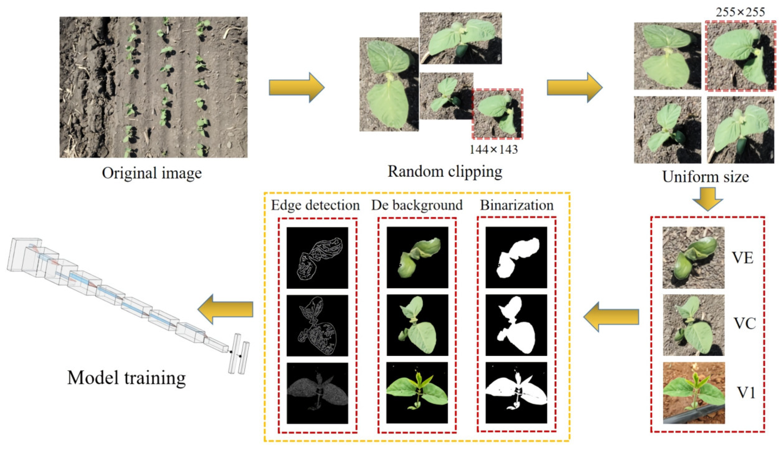
2.2. Dataset Construction

One-thousand original images were selected for each location. The required sample images were cut by manual clipping, and Photoshop software was used to modify the images size to 255 × 255 × 3. Effective image enhancement increases the number of training samples and the diversity of image data. Image datasets for three growth periods of soybean seedlings were constructed by adjusting image brightness, contrast, flip, and random rotation. There were 9000 images in the datasets, 3000 images in each period. As shown in

Table 1. Distribution of image datasets.

Period	Number of Training Set Images	Number of Testing Set Images	Image Label
VE	2250	750	0
VC	2250	750	1
V1	2250	750	2

, the training and testing set were divided by 3:1, with labels to distinguish them.

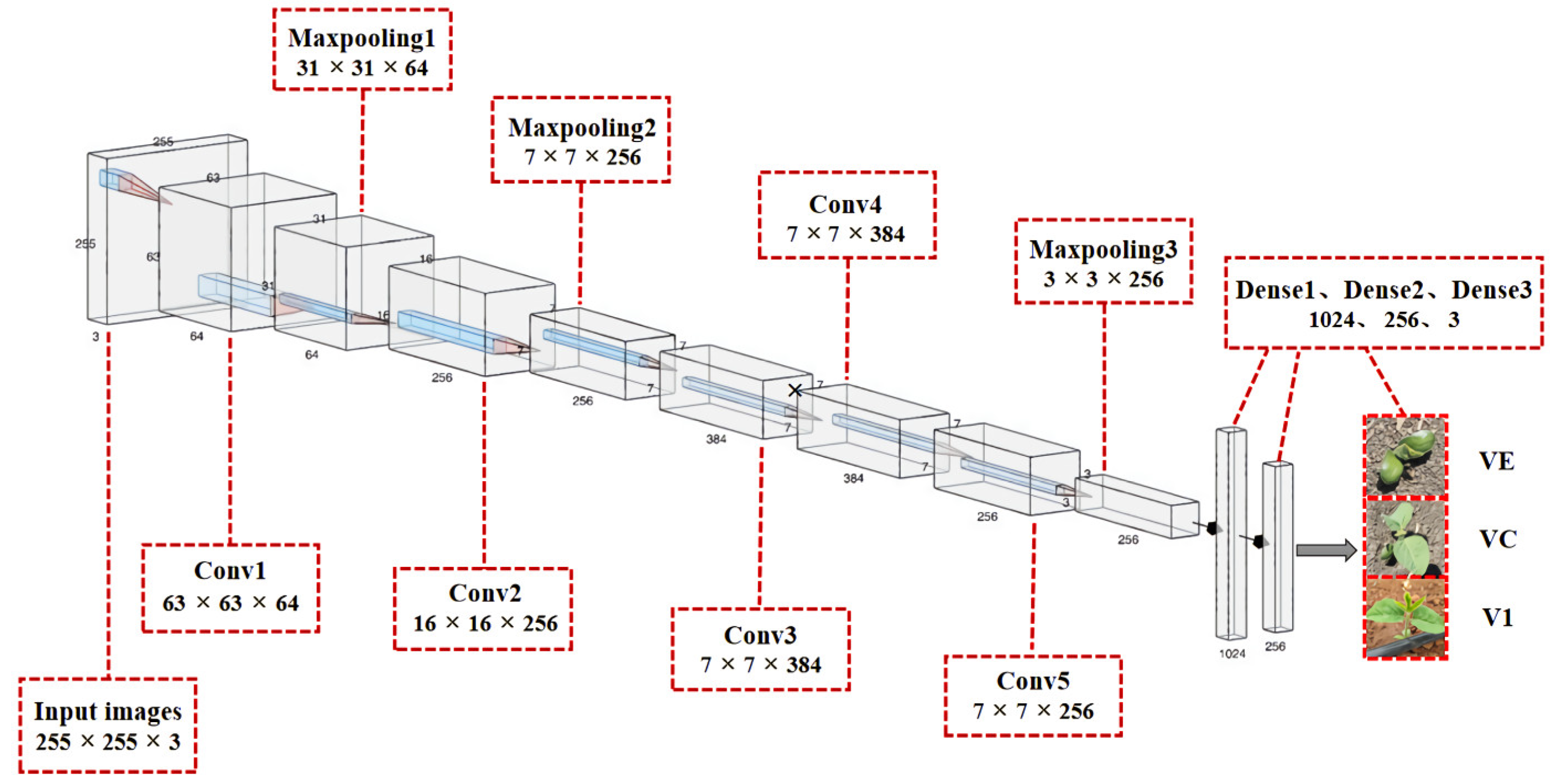
2.3. Model Establishment

AlexNet is a typical model in convolutional neural network with good classification performance [21]. Based on the AlexNet, the soybean seedling growth period discrimination model with self extracting features was established. AlexNet consists of 5 convolutional layers, 3 pooling layers, and 3 fully connected layers. Convolutional layers can effectively extract deeper feature information from certain regions of pixels in the images [22]. The convolution process is defined as follows:

$$Con{v}_{out}=\frac{Con{v}_{in}+2P-F_{conv}}{S_{conv}}+1$$

(1)

where Conv_out is the output image size, Conv_in is the input image size, F_conv is the convolution kernel size, P is the input images fill size, and S_conv is the convolution step.

Pooling layers are usually applied behind convolutional layers to further reduce computation. AlexNet uses max-pooling to reduce information loss by retaining the most prominent features in the images [23]. The max-pooling process is defined as follows:

$$M{p}_{out}=\frac{M{p}_{in}-F_{Mp}}{S_{Mp}}+1$$

(2)

where Mp_out is the output image size after max-pooling, Mp_in is the input images size in max-pooling, F_Mp is the convolution kernel size of max-pooling, and S_Mp is the pooling step.

The fully connected layers undertake the main calculation, store the final feature information, and realize image classification and prediction [24]. It is classified by Softmax and defined as follows:

$$S_r=\frac{exp\left(a_{rx}\right)}{{\sum }_{k=1}^{3}exp\left(a_{rk}\right)}$$

(3)

where S_r is the classification probability of the r-th soybean seedling belonging to the x-th growth period, a_rx is the product component of the r-th soybean seedling and the x-th growth period in the vector, a_rk is the product component of the r-th soybean seedling and the k-th growth period in the vector, and k is the number of growth periods (it is 3 in this study).

By improving the model structure, the identification accuracy, stability, and operation efficiency can be enhanced. The number of neurons in traditional AlexNet’s fully connected layer 1 and fully connected layer 2 is 4096. In this study, the fully connected layers were improved. The number of neurons in fully connected layer 1 and fully connected layer 2 was reduced to 1024 and 256 respectively, and fully connected layer 3 was set to 3. VE, VC, and V1 periods are classified by an improved model. The schematic diagram of fully connected layers before and after being improved is shown in Figure 1.

The final model was established to discriminate the growth periods of soybean seedlings as shown in Figure 2. The input image size was 255 × 255 × 3, and the feature map size of 3 × 3 × 256 was obtained. The convolution kernel size decreased from 7 to 5 and then to 3, whereas the feature map size was also reduced in half at layer 1, 2, and 5 by overlapping max-pooling. The image features had been extracted sufficiently to the fifth convolutional layers, and the classification results were obtained through the fully connected layers.

The training and testing of convolutional neural network adopted TensorFlow 2.5 deep learning framework and Keras module. Anaconda software, CUDA architecture, cuDNN development library, and Pycharm were applied. The processor was Inter(R) Core(TM)i5-1035G1 CPU @1.00GHz 1.19; the running environment was Windows 10 system; and the display adapter parameters were Inter(R) UHD Graphics, NVIDIA GeForce MX350.

2.4. Model Optimization

A large number of parameters need to be specified in the training of a convolutional neural network, and different sensitivity to various parameters lead to different experimental results. Hyperparameter is an important part of the model, which needs to be set before training. As a tuning parameter, it has the characteristics of a parameter and needs to be set manually. Different datasets and models have different applicable hyperparameters, so it is necessary to select appropriate hyperparameters through experimental design to obtain the optimal model. Improper setting of the learning rate will lead to model training shock or even divergence. In AlexNet’s fully connected layer 1 and fully connected layer 2, dropout is introduced to prevent the model from overfitting. Some nodes in the neural network will be closed and no longer communicate with each other, which can reduce the network complexity, make the network generalization ability stronger, and speed up the operation. Batch size is the size of each batch of data; by selecting a suitable batch size, the model training speed can be accelerated and the accuracy can be improved. Batch size to the power of 2 can speed up the calculation process [25].

Consequently, a single-factor experiment was designed to determine the value range of the hyperparameters. Learning rate, dropout, and batch size were selected as influencing factors. The experiment was conducted with learning rate (0.0001, 0.001, 0.0025, 0.005, 0.01) [26,27], dropout (0.5, 0.6, 0.7, 0.8, 0.9) [28], and batch size (16, 32, 64, 128, 256) [9], and Adam was selected as the AlexNet optimization algorithm.

A complex environment background will make a difference in the model feature extraction effect. The datasets constructed from binary images, background-removed images, and edge detection images were used as the model input for experiments. By comparing the classification results of different types of image datasets, the optimal image datasets were determined; the experimental flow chart is shown in Figure 3.

3. Results

3.1. Evaluating Indicator

The model performance is evaluated by accuracy and average accuracy. In the process of model training, the operation stability is explored by setting the number of iterations. In this work, the iterations number was 500, and the model will get a classification accuracy after each iteration. The calculation equation of model accuracy and average accuracy is as follows:

$$A=\frac{N_C}{N_T}\times 100\%$$

(4)

$$AA=\frac{e_T}{e}\times 100\%$$

(5)

where A is accuracy; N_C is quantity with correct classification; N_T is quantity of all samples; AA is average accuracy; e is epoch; e_T is sum of classification accuracy after each iteration.

3.2. Analysis of Hyperparameters Combination Experiment

The model was trained with a batch size of 32; dropout of 0.5; and learning rate of 0.01, 0.005, 0.0025, 0.001, and 0.0001, and the learning rate was 0.001 > 0.0001 > 0.01 > 0.005 > 0.0025. With the learning rate of 0.001; batch size of 32; and dropout of 0.5, 0.6, 0.7, 0.8, and 0.9, the dropout 0.5 > 0.8 > 0.6 > 0.7 > 0.9 was obtained. With the learning rate of 0.001 and dropout of 0.5, the batch size was 16, 32, 64, 128, and 256 to train the model, which was obtained as 32 > 128 > 64 > 256 > 16. The single-factor experiment results of hyperparameters are shown in Figure 4.

According to the single-factor experiment results of hyperparameters, a learning rate of 0.001, 0.0001, 0.005, 0.01; dropout of 0.5, 0.6, 0.7, 0.8; and batch size of 32, 64, 128, 256 were selected to arrange the combination test. The experimental design and results are shown in

Table 2. Experimental design and results.

Serial Number		Factors		Accuracy
	Learning Rate	Dropout	Batch Size
1	0.001	0.5	32	98.63%
2	0.001	0.6	64	98.77%
3	0.001	0.7	128	98.39%
4	0.001	0.8	256	97.12%
5	0.0001	0.5	64	99.47%
6	0.0001	0.6	32	99.58%
7	0.0001	0.7	256	88.25%
8	0.0001	0.8	128	99.14%
9	0.005	0.5	128	68.44%
10	0.005	0.6	256	40.11%
11	0.005	0.7	32	36.52%
12	0.005	0.8	64	37.63%
13	0.01	0.5	256	66.98%
14	0.01	0.6	128	39.08%
15	0.01	0.7	64	47.25%
16	0.01	0.8	32	43.42%

.

From the experiment results, the model corresponding to experiment 6 had the highest average classification accuracy of 99.58%. The best classification of soybean seedlings images was achieved with this hyperparameter combination. The convergence speed and stability are also the key to judge the performance of the model. According to the experiment results, the model performance before and after improvement were compared under the hyperparameter combination. The results are shown in Figure 5.

When the number of neurons in fully connected layer 1 and fully connected layer 2 was 4096, the average accuracy of the model was 99.53%, the average loss was 0.0209, and the running time was 0.55 s/step. While the average accuracy was 99.58%, the average loss was 0.0132, and the running time was 0.41 s/step when the number of fully connected layer 1 and fully connected layer 2 neurons were 1024 and 256, respectively. By comparing the two groups of experiment results, the improved model was superior to the original model in terms of running time, average loss, and average accuracy. The improved model started to converge at about 20 iterations, with fast convergence, stable operation, and less overfitting. Based on the above results, the optimal hyperparameter combination of the model was a learning rate of 0.0001, dropout of 0.6, and batch size of 32.

3.3. Performance Comparison of Different Image Datasets

Canny operator can effectively eliminate information irrelevant to image edges, so that morphological features and texture features can be completely preserved. After removing the background from the original images, all color features except for the soybean seedlings can be suppressed more obviously. Complex backgrounds were removed to make soybean seedlings more prominent. Binary allowed soybean seedlings to be screened out, but only the external morphological characteristics were retained. Several different image datasets were trained by the convolution neural network, and the model performance comparison is shown in

Table 3. Model performance comparison.

Datasets	Running Time	Average Loss	Average Accuracy
RGB Images	0.41 s/step	0.0132	99.58%
Binary Images	1.21 s/step	0.0978	94.53%
Background-removed Images	0.54 s/step	0.0123	99.61%
Canny Edge Detection Images	1.13 s/step	0.0294	99.52%

.

The results showed that the complexity of image background affected the model training. The average classification accuracy of the model for RGB images was 99.58%, with the shortest running time in the complex environment of soybean fields. The average classification accuracy of background-removed images was 99.61%, which was 0.03% higher than RGB images, but the running time was increased by 0.13 s/step, and the pre-processing took plenty of time, which increased the workload. Thus, from multiple perspectives of model performance and application efficiency, RGB images can meet the demand of discriminating soybean growth periods in actual agricultural production.

3.4. Field Experiment Validation

As a new method to obtain field data, an unmanned aerial vehicle (UAV) can quickly obtain images of large plots in a short time. It can avoid the error caused by manual shooting and effectively make up for the shortcomings of traditional image acquisition methods, with the advantage of high throughput [29]. More than 800 mu of No. 15 in Jianshan Farm with high hills, flat slopes, slopes, and other landforms was taken as the experiment site. According to the terrain difference and crop growth habits, DJI P4 Multispectral UAV was used to select representative locations to collect a large number of images. The UAV flight height was 5 m, the original images were 1600 × 1300 pixels, and the image enhancement and acquisition methods remained the same as before. Figure 6 shows the soybean seedling images in different growth periods under standard conditions, and the datasets include 3000 images.

AlexNet was used to train and test the RGB images of the UAV, and the model performance is shown in Figure 7. The average classification accuracy was 99.35%, the average loss was 0.0328, and the running time was 0.47 s/step.

Images were collected in the natural environment of the field, and datasets containing 1000 images were constructed to validate the practical application of the model, in which the images were not processed in any way. The classification accuracy was 90.81% in VE, 91.82% in VC, and 92.56% in V1, with an average classification accuracy of 91.73% and a single image recognition time of about 21.9 ms. The model combined with UAV field images allows for the accurate identification of soybean seedling growth periods.

4. Discussion

Many researchers have studied crop recognition and classification by improving the AlexNet. Different crop types and characteristics will affect the model recognition accuracy. Accordingly, recognition time, stability, and structural complexity are also criteria for evaluating the model. The recognition accuracy of kiwifruit in a complex environment by Mu et al. [30] was 96.00%, and the recognition time of a single image was about 1 s, but the recognition time of a single image of a soybean seedling was about 21.9 ms. Zhang et al. [31] realized the leaf classification of five plants by modifying different parameters of the AlexNet structure, with an accuracy of more than 99%. The model tended to be stable after 25 training times, whereas the soybean seedling recognition tended to be stable after 20 training times. Xiao et al. [32] showed 98.92% accuracy of rice pest identification, with an average loss of 0.03, whereas the average loss in soybean seedlings was 0.0132. Dong et al. [33] improved the classification model for nine strawberry pests and diseases, which increased the training time compared to the pre-improvement, whereas the improved soybean seedlings identification model saved 25.46% of the training time. The identification of heat damage stress in tomato seedlings was carried out by Wang et al. [34], with an average accuracy of 98.8%. Ni et al. [35] classified different types of peanut pods, with a maximum accuracy of 88.76%. The above comparative analysis showed that the discrimination of soybean growth periods using the improved AlexNet network has been improved in terms of recognition time, accuracy, and stability.

Research has been carried out for the identification of crop growth periods using sensors of different scales. Li [36] acquired winter wheat visible images by a near-earth end sensor, and used the improved Faster R-CNN to achieve the recognition of three growth periods with an average accuracy of 96%. Fu et al. [37] used UAV to identify four growth periods of maize by Swin Transformer model, and the test accuracy was 98.7% with a single image recognition time of 89.7 ms. Using satellite remote sensing images and based on the decision tree algorithm, Xu [38] achieved the identification of five growth periods of winter wheat, with the highest recognition accuracy of 86%. The crop images acquired by the near-ground end sensor are more accurate, but the coverage is smaller. Satellite remote sensing has a large coverage, but low accuracy. The advantage of UAV is that it can not only ensure certain accuracy, but also cover a large range. It has been tested as a high-throughput crop information detection tool [39]. For soybean growing period recognition, the test accuracy reached 99.35%, and still achieved good results in the actual field trial verification, with an accuracy of 91.73%, and it still has room for improvement. The identification model proposed in this study can provide decisions for management measures to be taken during different growth periods of soybean. It plays an important role in scientific and careful fertilizer application; the rational and timely use of pesticides to achieve yield preservation; and, to some extent, yield increase.

Based on this model, soybean VE, VC, and V1 periods were identified, and various control measures are still needed to ensure efficient and high-quality soybean growth in V2, V3, and subsequent growth periods. With the gradual vigorous growth, the soybean seedlings will overlap with each other and be sheltered by leaves. In this research, the early stages of soybean growth were identified, so the model did not consider the above phenomena, which became the key and difficult problem in the follow-up research. The model can be further improved and optimized and tried to be studied in combination with other algorithms.

5. Conclusions

In view of the importance of soybean growth period identification for timely management and control measures, the soybean seedling growth period identification model was constructed. By improving the fully connected layer structure of the AlexNet, and optimizing the selection of learning rate, dropout, and batch size, the identification of VE, VC, and V1 of soybean seedlings was realized. Through improving and optimizing the model, the simplified fully connected layer structure of 1024 and 256 was determined. The optimal combination of hyperparameters with a learning rate of 0.0001, dropout of 0.6, and batch size of 32 was determined. The average classification accuracy of the model was 99.58%, the average loss was 0.0132, and the running time was 0.41 s/step. Compared with the model before improvement, the performance of the model was improved by 0.05%, 0.0077, and 0.14 s/step respectively. The model was trained by UAV RGB images and verified in the field. The classification accuracy was 90.81% in VE, 91.82% in VC, and 92.56% in V1, with an average classification accuracy of 91.73%. It provides a new idea and method for the accurate and rapid identification of soybean seedling growth periods in the complex field environment, and offers a theoretical basis and technical support for agricultural managers to take timely measures in the corresponding growth periods of soybean.

References

1. Soltani, A.; Robertson, M.J.; Torabi, B.; Yousefi-Daz, M.; Sarparast, R. Modelling seedling emergence in chickpea as influenced by temperature and sowing depth. Agric. For. Meteorol. 2006, 138, 156–167. [Google Scholar] [CrossRef]
2. Guan, H.; Liu, M.; Ma, X. Automatic soybean disease diagnosis model based on image correction technology. J. Jiangsu Univ. Nat. Sci. Ed. 2018, 39, 409–413. [Google Scholar]
3. Lan, Y.; Deng, X.; Zeng, G. Advances in diagnosis of crop diseases, pests and weeds by UAV remote sensing. Smart Agric. 2019, 1, 1. [Google Scholar]
4. Lv, S.; Li, D.; Xian, R. Research status of deep learning in agriculture of China. Comput. Eng. Appl. 2019, 55, 24–33. [Google Scholar]
5. Liu, D.; Li, S.; Cao, Z. State-of-the-art on deep learning and its application in image object classification and detection. Comput. Sci. 2016, 43, 13–23. [Google Scholar]
6. Li, M.; Wang, J.; Li, H.; Hu, Z.; Yang, X.; Huang, X.; Zeng, W.; Zhang, J.; Fang, S. Method for identifying crop disease based on CNN and transfer learning. Smart Agric. 2019, 1, 46–55. [Google Scholar]
7. Hamuda, E.; Glavin, M.; Jones, E. A survey of image processing techniques for plant extraction and segmentation in the field. Comput. Electron. Agric. 2016, 125, 184–199. [Google Scholar] [CrossRef]
8. Szegedy, C.; Liu, W.; Jia, Y.; Sermanet, P.; Reed, S.; Anguelov, D.; Erhan, D.; Vanhoucke, V.; Rabinovich, A. Going deeper with convolutions. In Proceedings of the 2015 IEEE Conference on Computer Vision and Pattern Recognition (CVPR), Boston, MA, USA, 7–12 June 2015; pp. 1–9. [Google Scholar]
9. Shao, Z.; Yao, Q.; Tang, J.; Li, H.; Yang, B.; Lv, J.; Chen, Y. Research and development of the intelligent identification system of agricultural pests for mobile terminals. Sci. Agric. Sin. 2020, 53, 3257–3268. [Google Scholar]
10. Brahimi, M.; Boukhalfa, K.; Moussaoui, A. Deep learning for tomato diseases: Classification and symptoms visualization. Appl. Artif. Intell. 2017, 31, 299–315. [Google Scholar] [CrossRef]
11. Arif, M.; Tahir, F.; Fatima, U.; Nadeem, S.; Mohyuddin, A.; Ahmad, M.; Maryum, A.; Rukh, M.; Suffian, M.; Sattar, J. Novel synthesis of sensor for selective detection of Fe+ 3 ions under various solvents. J. Indian Chem. Soc. 2022, 99, 100754. [Google Scholar] [CrossRef]
12. Hou, J.; Yao, E.; Zhu, H. Classification of castor seed damage based on convolutional neural network. Trans. Chin. Soc. Agric. Mach. 2020, 51, 440–449. [Google Scholar]
13. Zhao, Z.; Song, H.; Zhu, J.; Lu, L.; Sun, L. Identification algorithm and application of peanut kernel integrity based on convolution neural network. Trans. Chin. Soc. Agric. Eng. 2018, 34, 195–201. [Google Scholar]
14. Niu, X.; Gao, B.; Nan, X.; Shi, Y. Detection of tomato leaf disease based on improved DenseNet convolutional neural network. Jiangsu J. Agric. Sci. 2022, 38, 129–134. [Google Scholar]
15. Zhou, Q.; Ma, L.; Cao, L.; Yu, H. Identification of tomato leaf diseases based on improved lightweight convolutional neural networks MobileNetV3. Smart Agric. 2022, 4, 47–56. [Google Scholar]
16. Shen, Y.; Yin, Y.; Zhao, C.; Li, B.; Wang, J.; Li, G.; Zhang, Z. Image recognition method based on an improved convolutional neural network to detect impurities in whea. IEEE Access 2019, 7, 162206–162218. [Google Scholar] [CrossRef]
17. Wu, B.; Zheng, G.; Chen, Y. An improved convolution neural network-based model for classifying foliage and woody components from terrestrial laser scanning data. Remote Sens. 2020, 12, 1010. [Google Scholar] [CrossRef] [Green Version]
18. Arif, M.; Rauf, A.; Tahir, F.; Saeed, A.; Nadeem, S.; Mohyuddin, A. Synthesis and optical study of highly sensitive calix [4] based sensors for heavy metal ions detection probes. Chem. Data Collect. 2022, 42, 100956. [Google Scholar] [CrossRef]
19. Fan, X.; Zhou, J.; Xu, Y.; Peng, X. Corn disease recognition under complicated background based on improved convolutional neural network. Trans. Chin. Soc. Agric. Mach. 2021, 52, 210–217. [Google Scholar]
20. Xu, J.; Shao, M.; Wang, Y.; Han, W. Recognition of corn leaf spot and rust based on transfer learning with convolutional neural network. Trans. Chin. Soc. Agric. Mach. 2020, 51, 230–236. [Google Scholar]
21. Li, Y.; Dong, H. Classification of remote-sensing image based on convolutional neural network. CAAI Trans. Intell. Syst. 2018, 13, 550–556. [Google Scholar]
22. Huang, L.; Shao, S.; Lu, X.; Guo, X.; Fan, J. Segmentation and registration of lettuce multispectral image based on convolutional neural network. Trans. Chin. Soc. Agric. Mach. 2021, 52, 186–194. [Google Scholar]
23. Yu, P.; Zhao, J. Image recognition algorithm of convolutional neural networks based on matrix 2-norm pooling. J. Graph. 2016, 37, 694–701. [Google Scholar]
24. Basha, S.; Dubey, S.; Pulabaigari, V.; Mukherjee, S. Impact of fully connected layers on performance of convolutional neural networks for image classification. Neurocomputing 2020, 378, 112–119. [Google Scholar] [CrossRef] [Green Version]
25. Zhao, L.; Hou, F.; Lv, Z.; Zhu, H.; Ding, X. Image recognition of cotton leaf diseases and pests based on transfer learning. Trans. Chin. Soc. Agric. Eng. 2020, 36, 184–191. [Google Scholar]
26. Zhang, R.; Li, Z.; Hao, J.; Sun, L.; Li, H.; Han, P. Image recognition of peanut pod grades based on transfer learning with convolutional neural network. Trans. Chin. Soc. Agric. Eng. 2020, 36, 171–180. [Google Scholar]
27. Long, M.; Ouyang, C.; Liu, H.; Fu, Q. Image recognition of Camellia oleifera diseases based on convolutional neural network & transfer learning. Trans. Chin. Soc. Agric. Eng. 2018, 34, 194–201. [Google Scholar]
28. Yang, G.; Bao, Y.; Liu, Z. Localization and recognition of pests in tea plantation based on image saliency analysis and convolutional neural network. Trans. Chin. Soc. Agric. Eng. 2017, 33, 156–162. [Google Scholar]
29. Zhu, B.; Li, M.; Liu, F.; Jia, A.; Mao, X.; Guo, Y. Modeling of canopy structure of field-grown maize based on UAV images. Trans. Chin. Soc. Agric. Mach. 2021, 52, 170–177. [Google Scholar]
30. Mu, L.; Gao, Z.; Cui, Y.; Li, K.; Liu, H.; Fu, L. Kiwifruit detection of far-view and occluded fruit based on improved AlexNet. Trans. Chin. Soc. Agric. Mach. 2019, 50, 24–34. [Google Scholar]
31. Zhang, W.; Wen, J. Research on leaf image identification based on improved AlexNet neural network. In Proceedings of the 2nd International Conference on Signal Processing and Computer Science (SPCS 2021), Qingdao, China, 20–22 August 2021. [Google Scholar]
32. Xiao, X.; Yang, H.; Yi, W.; Wan, Y.; Huang, Q.; Luo, J. Application of improved AlexNet in image recognition of rice pests. Sci. Technol. Eng. 2021, 21, 9447–9454. [Google Scholar]
33. Dong, C.; Zhang, Z.; Yue, J.; Zhou, L. Classification of strawberry diseases and pests by improved AlexNet deep learning networks. In Proceedings of the 13th International Conference on Advanced Computational Intelligence (ICACI), Wanzhou, China, 14–16 May 2021; Volume 5, pp. 14–16. [Google Scholar]
34. Wang, X.; Wu, Z.; Sun, Y.; Zhang, X.; Wang, Y.; Jiang, Y. Intelligent identification of heat stress in tomato seedlings based on chlorophyll fluorescence imaging technology. Trans.Chin. Soc. Agric. Eng. 2022, 38, 171–179. [Google Scholar]
35. Ni, J.; Yang, H.; Li, J.; Han, Z. Variety identification of peanut pod based on improved AlexNet. J. Pean. Sci. 2021, 50, 14–22. [Google Scholar]
36. Li, Y. Research on classification and recognition of growing period of winter wheat in central China plain based on deep feature learning and multi-level R-CNN. North China Univ. Water Resour. Electr. Power. 2021, 3, 1–58. [Google Scholar]
37. Fu, L.; Huang, H.; Wang, H.; Huang, S.; Chen, D. Classification of maize growth stages using the Swin Transformer model. Trans. Chin. Soc. Agric. Eng. 2022, 38, 191–200. [Google Scholar]
38. Xu, D.; Zhao, J.; Li, N. On scattering characteristics of winter wheat at different phenological period based on Sentinel-1A SAR images. In Proceedings of the IET International Radar Conference (IET IRC 2020), online, 4–6 November 2020; pp. 1478–1482. [Google Scholar]
39. Feng, A.; Zhou, J.; Vories, E.; Sudduth, K.A. Evaluation of Cotton Emergence Using UAV-Based Narrow-Band Spectral Imagery with Customized Image Alignment and Stitching Algorithms. Remote Sens. 2020, 12, 1764. [Google Scholar] [CrossRef]
Figure 1. Schematic diagram of fully connected layers before and after being improved.
Agronomy 12 02991 g001
Figure 2. Discrimination model of soybean seedlings growth periods.
Agronomy 12 02991 g002
Figure 3. Experimental flow chart.
Agronomy 12 02991 g003
Figure 4. Single-factor test results of hyperparameters.
Agronomy 12 02991 g004
Figure 5. Comparison of model performance before and after improvement: (a) change trend of model accuracy before improvement; (b) change trend of model loss before improvement; (c) change trend of model accuracy after improvement; (d) change trend of model loss after improvement.
Agronomy 12 02991 g005
Figure 6. Soybean seedling images of different growth periods.
Agronomy 12 02991 g006
Figure 7. Model performance analysis: (a) change trend of model accuracy; (b) change trend of model loss.
Agronomy 12 02991 g007