Intelligent Weed Management Based on Object Detection Neural Networks in Tomato Crops

Abstract

As the tomato (Solanum lycopersicum L.) is one of the most important crops worldwide, and the conventional approach for weed control compromises its potential productivity. Thus, the automatic detection of the most aggressive weed species is necessary to carry out selective control of them. Precision agriculture associated with computer vision is a powerful tool to deal with this issue. In recent years, advances in digital cameras and neural networks have led to novel approaches and technologies in PA. Convolutional neural networks (CNNs) have significantly improved the precision and accuracy of the process of weed detection. In order to apply on-the-spot herbicide spraying, robotic weeding, or precise mechanical weed control, it is necessary to identify crop plants and weeds. This work evaluates a novel method to automatically detect and classify, in one step, the most problematic weed species of tomato crops. The procedure is based on object detection neural networks called RetinaNet. Moreover, two current mainstream object detection models, namelyYOLOv7 and Faster-RCNN, as a one and two-step NN, respectively, were also assessed in comparison to RetinaNet. CNNs model were trained on RGB images monocotyledonous (Cyperus rotundus L., Echinochloa crus galli L., Setaria verticillata L.) and dicotyledonous (Portulaca oleracea L., Solanum nigrum L.) weeds. The prediction model was validated with images not used during the training under the mean average precision (mAP) metric. RetinaNet performed best with an AP ranging from 0.900 to 0.977, depending on the weed species. Faster-RCNN and YOLOv7 also achieved satisfactory results, in terms of mAP, particularly through data augmentation. In contrast to Faster CNN, YOLOv7 was less precise when discriminating monocot weed species. The results provide a better insight on how weed identification methods based on CNN can be made more broadly applicable for real-time applications.

1. Introduction

Tomato (Solanum lycopersicum L.) is one of the most important crops worldwide. The world production of tomatoes is around 170.8 million tons. China is the largest producer of tomatoes, and it represents 31% of the total production around the world. They are followed very closely, with second and third place, in terms of production, by India and the United States. Spanish production is around more than 4 million tons, ranking 11th among the countries with the highest tomato production [1]. However, the most problematic weeds for this crop put its production at risk, competing for water, light, nutrients, and physical space [2]. Besides, there is the problem of consumer acceptance worldwide regarding pesticide usage in the agri-food chain [3]. Therefore, using herbicides will be a challenging approach under increasing political and social pressure [4]. The reduction of herbicides, insecticides, and fungicides is a major motivating force behind the current agricultural expert systems [5,6] to comply with EU Directive 2009/128/EC [7].

Weed management plays one of the most important roles in tomato crops. Nowadays, the conventional approach in weed management is herbicides sprayed over the entire crop area [8], even in free weed areas. Nevertheless, the density and composition of weeds are not uniform throughout the field, with spatial and temporal variation [9]. Site-specific weed management (SSWM) could achieve a better precision of weed treatment with economic and environmental benefits leading to better food quality [10]. SSWM is achieved by applying a treatment only on the weed patches (e.g., using nozzles that open and close on command). This procedure could be complemented using the specific or most effective active ingredient for each weed species or a mixture of active ingredients. A system integrating SSWM and multi-species weed detection could achieve effective control of the most problematic weed species in tomato crops through the automatic selection of the herbicide to be applied. This approach could reduce the herbicide residues in the food chain. Thus, leading to safer agricultural products for the consumer and the environment and a more sustainable agriculture that is able to comply with EU (Directive 2009/128/EC) policies, such as Green Deal or from Farm to Fork.

Currently, new tools such as deep learning (DL) are helping to reach the aforementioned sustainable goals. This tool has shown promising and potential results in several research areas. Regarding agriculture, DL learning usage has been rapidly increasing since 2016 [11]. Convolutional neural networks (CNN) represents the most used DL technique in digital agriculture with 42% of publications [11] with digital images as input. Thus, digital cameras and neural networks (NN) are presented as an innovative and promising method in many fields of agriculture, especially in plant detections [12]. Dyrmann et al. [4] collected six datasets from different research papers and trained a convolutional CNN to classify a set of 22 weed species. In this work, a classification accuracy between 82.4% and 88.2% was achieved. These results show the CNN potential for digital classifications of weed species. In a similar research by Dyrmann et al. [13], a total of 17 weed species in a corn field was detected and classified. Segmentation techniques were used to detect plant species with intersection over union metric (IoU) [14] values between 0.69 and 0.93 for weeds and corn plants. After the detection of the weeds, a CNN was used to classify the weeds species with an overall accuracy of 87%.

Considering the application in real agriculture situations, the network classification accuracy varied from 33% to 98%, with the latter being for sugar beet (Beta vulgaris L.). In 2017, dos Santos Ferreira et al. [15] implemented a developed CNN to detect weeds in soybean crop images, even discriminating between monocotyledonous and dicotyledonous weeds. It was presented with a dataset comprising 15,000 images of soybean, weeds, and soil. According to the results, a replication of AlexNet reached a 99.5% average accuracy for all analyzed images. Using a CNN, Sharpe et al. (2019) [16] proposed an approach to in situ online detection and sprayed Goosegrass (Eleusine indica L.) in a 5-leaf stage in greenhouses with promising results. Interestingly, Osorio et al. [17] compared three methods for weed estimation in lettuce crops using ground truth data from experts. The methods support vector machines (SVM), YOLOv3, and Mask R-CNN were combined with the NDVI index to extract non-photosynthetic objects. The models had an F₁-score of 88% and 94%, respectively, for weeds and crop detection. Chen et al. (2018) [18] created a dataset of 5187 images of 15 weed classes specific to cotton (Gossypium hirsutum L.) to assess 27 DL models through transfer learning, where RestNet101 showed the best F1 score (>99%). Peteinatos et al. [19,20] evaluated three CNN architectures (VGG16, Inception, and ResNet-50) to classify weeds in maize, sunflower, and potato crops using images captured from a ground-based vehicle and found that the VGG16 outscored the other two CNNs. Additionally, they determined that datasets for CNN-based weed classification should be more robust, useful, and diversified. Weed classification was also accomplished using image segmentation using CNN. More recently, in 2022, Subeesh et al. [21] selected four DL models (Alexnet, GoogLeNet, InceptionV3, Xception) based on the complexity and computational cost to identify weeds in bell peppers. They reported overall accuracies ranging from 94.5% to 97.7%. Inception V3 exhibited the best performance for detection in terms of precision, accuracy, and recall, even though Xception was the most complex and the deepest one.

In each case, the authors illustrated the potential for NN to be used in digital agriculture, based on their impressive classification capabilities. In selective weed management, it is important to know the species under the sprinkler to select the specific herbicides and the doses to be applied. Some of the works cited [17,21,22] only discriminated between two classes: crop vs. weeds or monocotyledonous vs. dicotyledonous [15]. Other authors [4,18,19] were able to classify between weed species, but only the results by species classification were reported, leaving aside the problem of weed detection in the field. However, these networks require two processes to detect the species of the weeds: a prior segmentation process to detect plants and then classify them by species [13]. With this approach, numerous limitations remain, including the requirement for large training datasets and slow run time [23].

Recently, a new NN has been developed to allow for greater detection and classification of objects. One of those models is RetinaNet [24], which is a single-stage object detector that can handle object location and classification in one step. The development of RetinaNet has allowed it to be applied in the agricultural field, where real-time detections of different types of vegetables were achieved [22]. RetinaNet has been successful in reducing the prediction time and increasing the detection accuracy in many fields [24].

YOLO model has always been one of the most popular models for object identification used by deep learning experts [25]. A faster region-based convolutional neural network (Faster RCNN) is also a standard detection model that has been researched for weed identification. Rahman et al. [26] evaluated one-step (YOLOv5, EfficientDet, RetinaNet) and two-step (Fast RCNN, Faster RCNN) object detection neural networks, demonstrating the best mAP for one-step networks, compared to two-step networks. The best accurate values mAP obtained were 0.76 for EfficientDet and 0.78 for RetinaNet. However, only three weed species were considered (i.e., Mollugo verticillata L., Ipomoea lacunosa L., and Amaranthus palmeri L.), leaving aside the monocotyledonous species and classification between species of the same botanical family.

In agriculture, the real-time application on the fields occurs when data collection (i.e., weed images), data processing (i.e., prediction), and spray decision occur at the same time as the tractor advances. Given the several times required for the training and prediction of the conventional NN models, the prediction speed in real-time application of herbicides is an issue to solve in selective weed management in real time [27,28]. The use of RetinaNet for weed detection is scarce, according to the bibliography consulted, and it has shown a great performance for achieving accuracy, such as two-step NN, but with the speed of one-step NN. In the last conference paper published [29] for this research team, a general analysis of the RetinaNet performance was carried out in the maize crops.

RetinaNet is a fast and accurate NN for exploring the prediction accuracy against the most aggressive weeds in tomato crops, since the single procedure (one-step) allows for detecting and classifying objects in one step. Furthermore, RetinaNet is fast and highly accurate among object detection networks [30]. The single procedure allows us to detect and classify objects in one step with fast predictions. This characteristic motivates this research to explore the prediction accuracy against the most aggressive weeds in tomato crops. This one-step algorithm allows for discriminating between species that are morphologically very similar, such as grasses weed (monocotyledons), even between species of the same family, i.e., Graminae weeds. Furthermore, this one-step architecture avoids prior segmentation to detect plants in the field. Thus, RetinaNet provides fast prediction models that could solve the problem of slow NN for real-time applications, while maintaining a satisfactory mean average prediction (mAP). Nonetheless, since computing processing capacity has increased over the years at a fast pace, Retinanet stands out as a potential network to be applied in real time weed management.

Due to the current developments and the required speed and accuracy needs of a novel procedure, based on object detection NN, RetinaNet was analyzed according to the precision, prediction time, and number of the trained parameters. The current study proposes a one-step detection and classification method discriminating between the most aggressive weed species in tomato crops (Solanum lycopersicum L.) under real and commercial production fields. Discriminating, morphologically similar species, such as the monocotyledonous weeds (Cyperus rotundus L., Echinochloa crus galli L., Setaria verticillata L.) and dicotyledonous weeds (Portulaca oleracea L., Solanum nigrum L.). This study also addresses the challenging discrimination between weeds of the same family with many similarities that only accentuates the confusion, i.e., Echinochloa crus galli L. and Setaria verticillata L. In addition, the target weeds, although seedlings, were under different early phonological stages.

Due to unstructured field conditions and the high biological variety of weeds, effective and reliable weed detection continues to be a tough task. Furthermore, the proposed methodology copes with an image dataset with a high variability not only with regard to the target weed species but also the image acquisition process. The dataset was enriched to provide the most faithful input to the NN, hence making up a more technically demanding dataset. Images were captured at different times of the day for several days. In this manner, different weather conditions and crops and weeds casting changing shadows altered the images background. Furthermore, in order to take a step further, the dataset was also enhanced by acquiring images in different land plots, hence providing different backgrounds, due to the varying soil conditions, i.e., different colors. In addition, RetinaNet was analyzed and compared, in terms of computational complexity, with two currently state-of-the-art object detectors: a two-step NN called Fast-er-RCNN and, particularly, YOLO as a one-step NN, according to the latest 7th version.

2. Materials and Methods

2.1. Image Acquisition

The selected fields for the experiments were in the province of Badajoz, Spain (39°1′14.42″–6°3′40.69″). All the images were collected on commercial fields under real uncontrolled illumination conditions during several days at different times, in order to capture different soil backgrounds, shadows, and illumination conditions. Tomato crop and the weeds were in the scene of the image. Additionally, weeds were in the line and interline crops. A large proportion of weeds in the crop line overlapped with tomato plants, especially in advanced growth stages. The images were taken in early stages of development, to coincide with the period of weed treatment. No herbicide spraying was carried out during the image acquisition or 10 days before. Each lot was processed following an “M” trajectory. Every 2 m, a zenithal image was taken from a height of 1.3 m. Five weed species, monocotyledonous (Cyperus rotundus L., Echinochloa crus galli L., Setaria verticillata L.) and dicotyledonous (Portulaca oleracea L., Solanum nigrum L.), were found in low growth stages, combined with crop plants (Solanum lycopersicum L.). The considered species are the most problematic tomato weeds in Spain [31]. The camera used was a Canon PowerShot SX540 HS with a spatial resolution of 5184 pixels × 3886 pixels. A shutter speed of 1/1000 was used, while the ISO was calibrated automatically to achieve a good image quality under the changing lighting conditions.

2.2. Image Pre-processing

A total of 1713 images were captured, in which the plant species were identified and manually labelled by weed science experts. LabelImg [32] was employed using the PascalVOC format [33] to export the corresponding XML files. This format saves the coordinates of the bounding boxes surrounding the objects. All bounding boxes defined by one image were saved in a single XML file. Each object saved the coordinates of the upper-left and lower-right corner (xmin, ymin, xmax, ymax), as well as the class name of the labelled object. Some examples of the data are shown in Figure A1. Seven plant species were categorized with the help of weed science experts, labelled according to the EPPO (European and Mediterranean Plant Protection Organization) code system. The labels are explained below: SOLNI for plants identified as the species Solanum nigrum L. (Figure A1a), POROL for plants identified as the species Portulaca oleracea L. (Figure A1b), SETIT for plants identified as the species Setaria verticillata L. (Figure A1c), ECHCG for plants identified as the species Echinochloa crus galli L. (Figure A1d), CYPRO for plants identified as the species Cyperus rotundus L. (Figure A1e), NR for species not recognised by the expert for their small size in the image (Figure A1f), LYPES for plants identified as the species Solanum lycopersicum L. (Figure A1g).

In order to evaluate the predictive potential of a model, it was necessary to perform these evaluations with data that had not been used for training, e.g., “new data for the model”. The dataset was split into 5 folders, with 342 images per folder. Four of them were used for the training and cross-validation processes (in each iteration, 3 folders belonged to the training set and 1 folder belonged to the validation set). The remaining folder was used for the validation set. Test prediction quality was assessed through mAP. Both the training set and test set were conducted using a GeForce GTX 1080 GPU. Captured image sizes could not be processed with the processing power of the GPU, requiring a reduction of their size. Thus, a scan of the images was performed, generating 74 smaller sub-images for each full image. Three parameters had to be selected: image height, image width, and overlap between one sub-image and the next. 3886 pixels for width, 1926 pixels for height, and an overlap of 1900 pixels were selected. Each XML that defined the plant labels in the original images was corrected accordingly, resulting in a new XML file for each sub-image. As a result of the scanning process, some bounding boxes that are in contact with edges of the sub-image might be cut, resulting in incomplete data. To avoid the use of this data for training, those boxes were eliminated. The large overlap specified for scanning allows that, if a plant is removed because it touches the edge, it will appear in the next sub-image, thereby ensuring that all the plants in the original images have a label on the training set. From these, any sub-image without bounding boxes was deleted. The labels were visually examined by experts who corrected labelling errors. After the scanning procedure, 10,607 bounding boxes were obtained (

Table 1. Labelling weed species by EPPO code (European and Mediterranean Plant Protection Organization). Number of labels by bounding boxes in the Training set, Test set, and Validation set.

Species	Label	Training Set	Test Set	Validation Set
Solanum nigrum L.	SOLNI	1917	383	821
Cyperus rotundus L.	CYPRO	1691	338	725
Echinochloa crus galli L.	ECHCG	895	179	384
Setaria verticillata L.	SETIT	157	31	67
Portulaca oleracea L.	POROL	506	506	101
Solanum lycopersicum L.	LYPES	799	160	342
Not recognised	NR	372	74	159

).

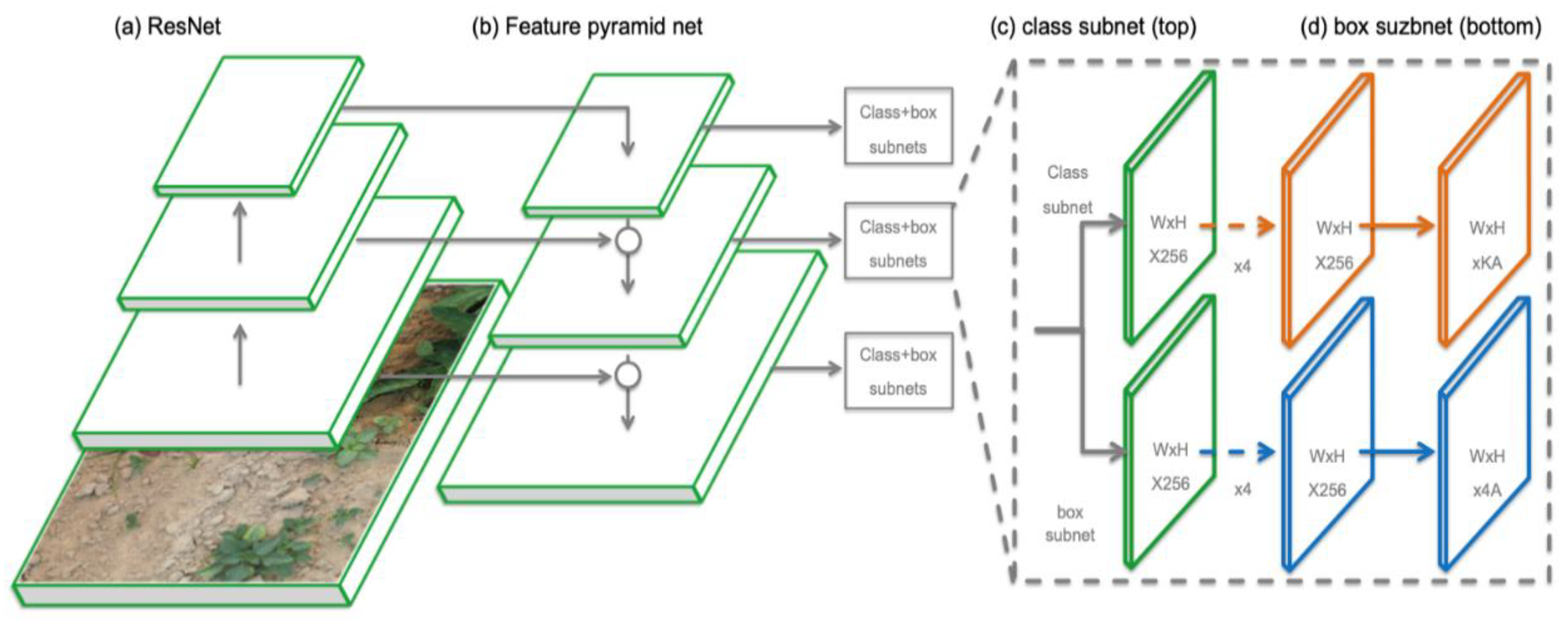
2.3. RetinaNet Object Detection Neural Network

Object detection is a powerful technique that can achieve successful plant and weed identification. The state-of-the-art object detectors can be collectively divided into two categories: (1) one-step detector and (2) two-step detectors [32,34]. The one step is a detection process and the second is the classification of these objects. RetinaNet is a one-step detector, a unified network composed of a backbone network and two task-specific subnetworks. The backbone is responsible for computing a convolutional feature map over an entire input image and is an off-the-self convolutional network. The first subnet performs convolutional object classification on the backbone output, whereas the second subnet performs convolutional bounding box regression. The two subnetworks feature a simple design for one-stage dense detection. Further details on the RetinaNet architecture are provided in Lin et al. [24] RetinaNet was selected among the object Detection networks as it has shown a good performance achieving accuracy like two-step networks but with the speed of single-step networks. Figure 1 shows a graphical representation of RetinaNet architecture.

2.4. Training Model

Weed and tomato plants were classified in seven different classes (SOLNI, CYPRO, ECHCG, SETIT, POROL, LYPES, NR). Training was made using the implementation proposed by Gaiser et al. [35]. The DL model used in this study was implemented using Keras 2.4.3 in Python 3.6.8 with the TensorFlow (2.3.0) back-end.

Collecting a large enough dataset for creating a unique DL method intended for a specific application is extremely time-consuming and virtually impossible. Therefore, DL methods commonly use a pre-trained computer vision model trained on a large training dataset, so-called transfer learning (TL) [5]. Using TL, feature extraction methods can be leveraged due to models trained on standard datasets; thus, object detection is finely tuned to the specific target [11]. The Resnet50 [36] model, as the backbone network, pre-trained model by TL with the COCO dataset, and with an initial learning rate of 1 × 10⁵, was used. For the training subsets, data augmentation [37] was also undertaken to avoid over-fitting and overcome the highly variable nature of target classification. The Keras [38] library was modified and improved for the data augmentation parameters, such as rotation, scale, illumination, perspective, and color. Specifically, rotation of up to 10°, a brightness shift of ±20%, a channel shift of ±30%, and a zoom of ±20%. Thus, 280 news bounding boxes per each annotation were performed, according to 35 rotations, 2 brightness shifts, 2 brightness shifts, and 2 zoom shifts. As the RetinaNet implementation needs to input images with their annotations (bounding boxes), they enter into the workflow unbalanced. However, in the script implementation, the bounding boxes entered into the backbone processed by under-sampling method [39], producing a balanced number of annotations to model training.

The training performance of the model was evaluated following the most accepted metric by the scientific community for Object Detection models: the Average Precision (AP) per class and the mAP is the mean between all classes. This metric evaluates both the detection and classification process. The way it does it is by evaluating the detection process with the Intersection over Union (IoU) metric. It is a measurement based on the Jaccard Index, a coefficient of similarity for two sets of data. In the Object Detection scope, the intersection IoU measures the overlapping area between the predicted bounding box and the ground-truth bounding box divided by the area of union between them, as illustrated in the Equation (1) and Figure 2.

$$IoU=\frac{area\left(Bp{\displaystyle \cap }Bgt\right)}{area\left(Bp{\displaystyle \cup }Bgt\right)}$$

(1)

Then the evaluation of the classification process was carried out by comparing the IoU with a given threshold (t = 0.5) and selecting the detection of highest confidence for each ground-truth bounding box. This way, each detection could be:

True positive (TP): A correct detection of plant species with the highest probability on a bounding box.

False positive (FP): An incorrect detection or a misplaced detection of plant.

False negative (FN): An undetected plant species.

The true negative result does not apply in the object detection context, because it is a background of images and, thereby, there would be an infinite number of bounding boxes that should not be detected within any given image. The general definition of average precision (AP) is the area under the curve of precision (P) × recovery (R), as shown in Equation (2). Then, considering Equations (3) and (4) for calculation of precision and recall, the AP is obtained [40].

$$\mathrm{AP}={{\displaystyle \int }}_1^{0}P\left(r\right)dr$$

(2)

$$Precision=\frac{TP}{TP+FP}$$

(3)

$$Recall=\frac{TP}{TP+FN}$$

(4)

RetinaNet was trained until the mAP of the training set of every class did not improve for 16 consecutive epochs. The parameters used for implementing RetinaNet were the following: 1 × 10⁵ as the learning rate, backbone model ResNet-50 pre-trained on the COCO dataset, 100 epochs to train, and 600 steps per epoch. Moreover, the backbone layers were frozen during training, the images were not resized, and option image augmentation was carried out as stated above. Furthermore, the batch size was 8 and the IoU threshold (t) selected was set at 0.5.

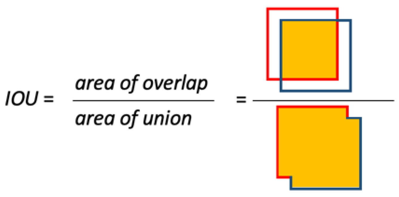
2.5. Fitness Evaluation

The training progress was evaluated epoch by epoch throughout AP metric per class for both test and validation sets. The training was carried out until the model converged. Hence, AP values did not improve epoch by epoch on the validation test. At this point in the training, the learning curves became asymptotic, and the model did not overfit. The overfitting issue arose when the statistical DL model learned the training data set so well that its performance on unseen data sets was inadequate. Thus, this signifies that the DL learning model adjusted very effectively to both the noise and signal included in the training data [41]. Therefore, overfitting indicated that the accuracy model was accurate for predicting the validation set image, but not new images, such as those in the test set. Therefore, once the training was finished, the real performance of the model was evaluated with images it had never seen for the model.

The first experiment seeks to evaluate the general prediction performance of the model to identify crop and weeds species under real field conditions. To achieve this goal, an analysis was carried out epoch-by-epoch with the mAP between all the classes. The second experiment was based on the same analysis as the first experiment. The objective was to evaluate which species were best using AP. RetinaNet was analyzed, in terms of computational complexity (speed prediction, i.e., detection and classification, number of trained parameters) along with two popular object detection frameworks: faster-RCNN as a two-step NN [42] and YOLOv7 as a one-step NN [43]. Hyper parameters settings for both Faster-RCNN and YOLOv7 remained the same as for RetinaNet to compare under homogeneous conditions. The third experiment showed a detection result of the most important groups of weeds, i.e., dicotyledonous and monocotyledonous plants. The mAP was calculated with the species of each group. The last experiment poses an analysis based on selective detection of weeds vs. crops on the dataset.

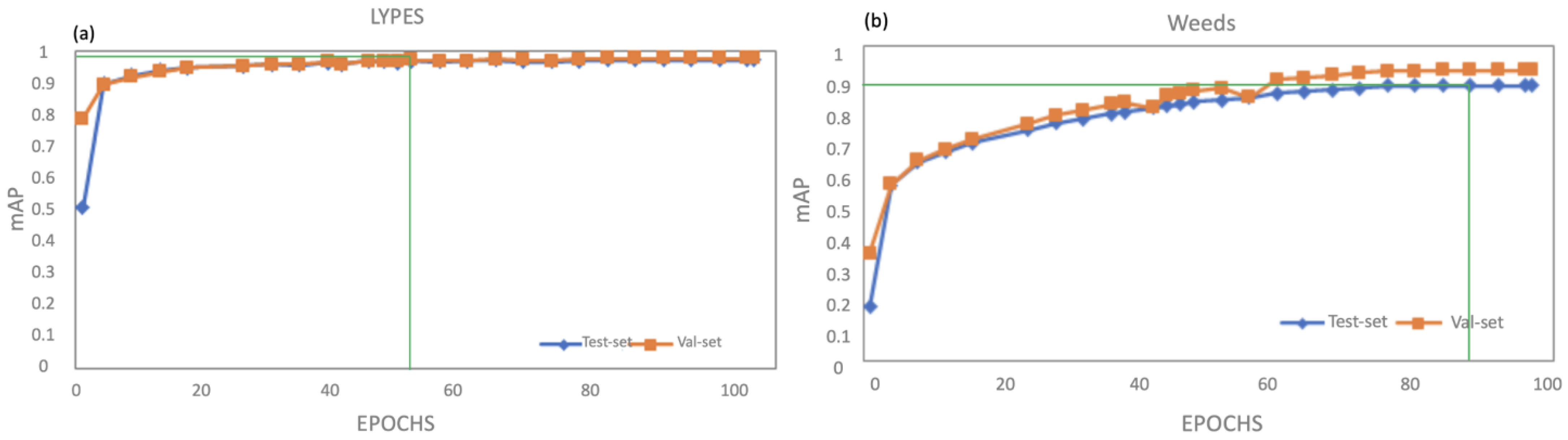
3. Results and Discussion

This study automatically classified six different species of weeds and crop, specifically: monocotyledonous (Cyperus rotundus L., Echinochloa crus galli L., Setaria verticillata L.), dicotyledonous (Portulaca oleracea L., Solanum nigrum L.), and the tomato crop (Solanum lycopersicum L.) under real field conditions. The training performance of the RetinaNet model, represented by mAP values per epoch, is shown in Figure 3, representing the validation set (rhombus data markers) and test set (square data markers). The best results for the first experiment were achieved in 85 epochs, and the trained model converges and obtains its maximum prediction value (mAP: 0.92755) over the validation set. The AP values per class are shown in

Table 2. Prediction mAP values on the test set per species identified by EPPO code as label.

Species	Label	AP
Solanum nigrum L.	SOLNI	0.9209
Cyperus rotundus L.	CYPRO	0.9322
Echinochloa crus galli L.	ECHCG	0.9502
Setaria verticillata L.	SETIT	0.9044
Portulaca oleracea L.	POROL	0.9776
Solanum lycopersicum L.	LYPES	0.9842
Not recognised	NR	0.8234
mAP	----	0.92755

, where the lowest value of AP occurs for the not recognised plant (NR) classes with 0.8234 AP value and the highest for the tomato crop class (LYPES) with a 0.9744 AP value.

An example of weed detection for qualitative evaluation in an image is shown in Figure 4. The detected plants are boxed and labeled with the confidence level. These tests results are presented with the value of IoU set to 0.5.

A model was trained to demonstrate which species is the best class detected. The training progress, by increasing the number of epochs until reaching the maximum precision on the validation set and the test set by species, is shown in Figure 5. The green line indicates the maximum average precision (AP) obtained on the vertical axis and the horizontal axis shows the first epoch when this AP is reached. Regarding the weed species, the best prediction was achieved for Portulaca oleracea L. (POROL), with 0.9842 AP value reached in epoch 85. The lowest AP value was for Setaria verticillata L. (SETIT), with 0.904 in epoch 82.

In addition, two species (Echinochloa crus-galli L., Setaria verticillata L.) of the same botanical family (Poaceae) were detected with 0.9502 and 0.9044 AP, respectively. As members of the same family, these species have similar morphological traits that make it extremely difficult for classification algorithms to discriminate. Particularly, the detection of Echinochloa crus-galli L. is relevant, due to well-known reported genetic resistance to herbicides [44,45]. For many years, weed control by herbicides was the most effective and efficient weed management system. Nevertheless, the use of herbicides with the same sites of action (i.e., physiological sites of attack) and generic herbicides to control a broad spectrum of weed species year-by-year has led to the problem of herbicide weed resistance [46].

The NR class obtained the lowest AP value, 0.8234, in epoch 86. This class contains examples of small weed seedlings that were not properly recognised by the experts, due to the small size in the images. The algorithm, on the other hand, was excellent at detecting small weeds of this type. These small weeds are at low stages of development, which allows for early weed control. Therefore, lower doses of herbicide in chemical control or less soil removal in mechanical control could be achieved. Previous research [19,37,42,44] has reported a great accuracy for weed detection. However, they properly work on big weed sizes and high-quality resolution images, which usually does not happen under real field conditions working in real time. Thus, real field conditions must be tested, in order to perform site-specific applications. Considering the detection results by the most important groups of the plants,

Table 3. Performance detection of the monocotyledonous and dicotyledonous weeds by mAP metric between each group.

Weed Group	Species Label	mAP
Dicotyledonous	SOLNI and POROL	0.9492
Monocotyledonous	CYPRO, SETIT and ECHCG	0.9533

shows the prediction performances of the model discriminating between dicotyledonous and monocotyledonous weeds.

This potential discrimination can be implemented in simple spraying and hoeing operations, when only the crop and weed need to be separated in digital images, or weed species can be grouped into classes of monocotyledonous weeds and dicotyledonous weeds. Hence, it might be a faster and more efficient treatment [47], since many commercial herbicides are intended to control groups of weeds such as broadleaf (monocotyledonous) and narrowleaf (dicotyledonous) herbicides. In this work, RetinaNet has managed to discriminate with a precision of 94% and 95% between monocotyledonous and dicotyledonous weeds, which can lead to more specific and effective spraying.

The classification of weeds (all species) vs. crops has a great impact because the model detects 98.4% of the tomato plants and 0.91% of the weed plants. Thus, under site-specific weed management or robotic technology [43,48,49], the model could spray herbicide only on the surface of the field where there are weeds avoiding spraying the crops. Therefore, this approach reduces herbicide use, compared to conventional farming, which involves uniform field application.

The results provided in Table 3 agree with those achieved by [50], utilizing high-resolution UAS-based RGB imagery to train YOLOv3 as a single-step architecture. However, the highest mAP score of 0.9148 and 0.8613 for monocot and dicot weeds were obtained at the 0.25 IoU threshold, instead of 0.5, as in this study. When the IoU was set at 0.5, the mAP decreased to 0.6337 and 0.4513. Although these values are lower, these results open a new way for identifying wees with field images in the challenging scenario of weeds in early phenological stages. As expected, the best values for mAP were achieved when the UAS imagery was acquired at 10 m above the ground level at both the 0.5 and 0.25 IoU. In contrast, the present approach managed to discriminate not only monocot and dicot weeds, but also within each group.

The results of the detection of weeds vs crop experiment are shown in Figure 6, which represents the maximum precision for the prediction of weeds species and crop plants. The results obtained were 0.9842 AP for tomato plants (LYPES) and 0.9118 mAP for weed plants (SOLNI, CYPRO, ECHCG, SETIT, POROL, NR). The LYPES class reached the maximum precision in early epochs (55), while the weed plants reached it in 84 epochs.

Previous studies focused only on classification of weed species have shown accuracies between 94% and 99.5%, depending on the selected neural network and the quality of training [12,15,19,51], leaving out detection analysis. Hence, the performance of two-stage and single-stage object detection models was assessed. The analysis of the three different CNN proposed in this study, i.e., RetinaNet, YOLOv7, and Faster-RCNN, provides a better insight to understand their strengths and weaknesses under the remaining challenge in DL to detect weeds robustly and accurately. Moreover, for the purpose of creating image-based weed identification for site-specific weed management, it is crucial to have a structured weed detection dataset with correct annotations and to thoroughly research weed detection methods. Numerous variables influence weed identification, including the intra- and inter-species variation in weed appearance traits, i.e., shape, size, color, and texture. The resemblance between weeds and crops and changes in field lighting conditions and soil backgrounds [26] have and influence as well. In order to cope with this issue, a diverse dataset that includes the necessary variance, according to the criteria stated in [52], was performed. Moreover, to ensure the quality of the data, every attempt was taken to remove low-quality original annotations.

In this manner, RetinaNet performs exceptionally well in predicting AP values based on weed species and crop. However, YOLOv7, despite being a fast NN, in terms of prediction the discrimination of monocot weeds, reveals its weakness. The explanation can be found due to detected false positives in the ECHCG class, likely transferred from false positives from SETIT and CYPRO classes. However, the detection of dicotyledon species is quite robust. YOLOv7 detects NR class effectively, as well, because YOLO has excellent object detection performance. Hence, it detects small objects, such as NR class, very well. Nevertheless, YOLOv7 may be correctly classifying them based solely on the size of the bounding box. However, this mismatch should be researched in future studies focusing on these monocot weeds species. Regarding the AP for Faster R-CNN, this model shows high precision for the general multi species classification, also for the monocotyledonous species. The lowest value has been obtained for SOLNI, this hypothesis is speculative and requires more research in this regard. In terms of accuracy, Faster R-CNN and RetinaNet show similar and excellent performance in detecting weed species (

Table 4. Prediction AP values on the validation set per Object Detection Model and species.

Label	RetinaNet	YOLOv7	Faster-RCNN
SOLNI	0.9209	0.8100	0.86755
CYPRO	0.9322	0.5533	0.90785
ECHCG	0.9502	0.9650	0.91056
SETIT	0.9044	0.6349	0.89502
POROL	0.9776	0.9323	0.92346
LYPES	0.9842	0.9530	0.96763
NR	0.8234	0.96735	0.97735

). However, the lower AP value of the SOLNI class can be explained due to the small size of the weed species in the images, hence being added as false positives in the NR class. Another possibility could be that the SOLNI class was below the threshold of 0.5 for the IoU.

On the other hand, the method of data augmentation produces data for DL models, it reduces the model reliance on training data and enhances its effectiveness for DL. When trained with new data supplied by data augmentation, deep learning models often perform better [53]. Furthermore, augmentation methods combat overfitting phenomenon, while improving the CNN test accuracy [54]. Thus, the distance between the training set and the validation set, and potentially the future testing sets, will be reduced, since the augmented data will represent a more complete collection of the possible data points [37]. Thus, to reduce the errors in detection and classification due to the different image conditions in the dataset, all CNN models improve the mAP, particularly YOLOv7 and Faster-RCNN (

Table 5. Comparison of the different models, including the data augmentation effect.

Neural Network	mAP	Speed Prediction Sec/Frame	Number of Trained Parameters
RetinaNet	0.90354	0.2354	39,336,702
RetinaNet and Augmentation	0.92755
YOLOv7	0.65346	0.0869	36,519,530
YOLOv7 and Augmentation	0.83085
Faster-RCNN	0.89135	1.2863	55,338,998
Faster-RCNN and Augmentation	0.92135

). YOLOv7 increases the accuracy of the detection, while simultaneously simplifying the structure of the prediction network and reducing the amount of time spent on detection. YOLOv7 is a very fast one-step network but less precise when there is a high variability in terms of classes. RetinaNet has the speed of one-step networks and the accuracy of two-step networks. Although RetinaNet has a high detection accuracy, its potential inability to execute real-time detection in applications is a result of the large number of parameters and large size of the model. However, with the advancement of technology, in terms of hardware and software, the application of RetinaNet as a one-step model might be feasible within the next few years.

The detecting procedure in the Faster R-CNN occurs in two steps. A regional proposal network analyzes the image with a feature extractor and generates a score for each proposal during this phase. These regression layers forecast the category and bounding box to which each regional recommendation bounding box belongs in the second phase. This results in a better virtually costless with regional proposal. On the basis of Faster R-CNN and high accuracy in object detection and classification, other networks have been constructed. However, Faster-RCNN requires more trained parameters, hence the speed prediction time is higher. Although YOLOv7 features a fast speed, it is not as accurate as the Faster R-CNN detection method in terms of detection accuracy. YOLOv6 is not accurate enough for object localization and has a low recall rate. After that, YOLO v7was proposed to improve YOLOv6 in several aspects. Normalization on convolution layers were added using a high-resolution classifier, along with convolution layers with anchor boxes, to predict bounding boxes, instead of the fully connected layers.

Moreover, the classification process is more difficult when the crop resembles weeds; hence, a large number of parameters are needed in the NN, combined with a high level of computational power [55]. The advantage of CNNs is the ability to create correlations and extrapolate and weigh new features independently [49,56]. There are two CNNs limitations in weed detection: the high-capacity data processing hardware and the long computing time in the training and prediction stage make it difficult to adopt, especially for real-time systems [19,57]. The effort required to train CNNs with plant species at various stages of development and under various environmental conditions is enormous, and it may necessitate the collaboration of several working groups [4,19]. Hall et al. [58] reduced the prediction and training CNN time by selecting labelling weed species in cotton, without significantly reducing classification accuracy.

Interestingly, Sapkota et al. [59] performed a cross-applicability study in cotton, soybean, and corn using two popular object detection frameworks, YOLOv4 and Faster R-CNN. These NN were assessed to detect weeds under two schemes: detecting at weed/crop level detection and weed species level detection. The authors achieved high AP between 0.83–0.88 values, in terms of discrimination between morning glories (dicots) grasses (monocots). However, the research did not consider the discrimination between species of monocotyledonous weeds, as presented in this study.

In addition, the RetinaNet prediction speed for 3886-pixel by 1926-pixels was 0.2354 s per image, which is slow for real time applications. Thus, prepossessing of the data is necessary to implement the system under field conditions. Although the data processing capacity of computers evolves at a great speed, real-time forecasts are not feasible yet. On the other hand, new self-labelling algorithms are being developed by the research team to increase the number of images. This work will include more weed species and growth stages, as well as increasing the amount of data per class. Regarding network configuration, the analysis of both performance and inference rate of other object detection networks is also planned. Furthermore, a greater amount of variability in the dataset images will be added to evaluate the combinations of the parameters to be adjusted from RetinaNet, as well as all combinations of parameters with different classification architectures (e.g., RestNet101, ResNet152, VGG, DenseNet, DffNet, MobilNet, SeNet). Thus, a higher accuracy, with lowering processing times, would be achievable.

Artificial perception and SSWM reduce herbicide use and the aggressiveness of mechanical treatments. Technologies for site-specific spraying highlight the potential of herbicide savings, which are up to 90% [60]. The herbicide reduction is significantly less, regardless of the spraying technology used [61]. Additionally, herbicide saving generates a greater protection of the environment, e.g., herbicide infiltration into groundwater, lowers risk of resistant weeds, and reduces agrochemical residues in the food chain [62]. In addition, the biodiversity of weed species and insects can also be increased, and rare weeds species can be protected by reducing the herbicide load on the environment [63,64]. Moreover, the European Commission has set a concrete strategic plan to reduce the use of chemicals, specifically 50% by 2030 (EU Green Deal), enhance biodiversity, and assist farmers in decision-making processes to increase farm sustainability within the borders of the Union. Nevertheless, it is still undefined whether a reduction in herbicide use could be feasible in different farming systems and situations [65]. A SSWM based on an automatic weed detection system could be a powerful tool to meet this challenging goal. The use of object detection networks could be very useful for smart spraying during herbicide applications, given that these networks can be integrated into treatment systems in real time and are capable of deciding what type of treatment is to be applied, with some commercial prototypes, such as the Blueriver case [29], combined with a real-time detection system on a commercial plant-by-plant applicator. All these systems are rapidly evolving and may be a response to the demand for reduced herbicide use and higher yields. In addition, the current study has obtained higher accuracy values than similar research [26] using RetinaNet (mAP values of 0.78, against 0.900–0.9 soil backgrounds 77 in the present paper). However, only three dicotyledonous weeds were considered in the cited paper, leaving aside the monocotyledonous species. Additionally, the classification between species of the same botanical family was not considered. This is a great challenge for the present study, since it was able to detect Echinochloa crus galli L. with 0.9502 of mAP and Setaria verticillata L. with 0.9044 of mAP. YOLOv7 and Faster-RCNN should be further explored, along with the promising RetinaNet performance, since the trade-off between improved accuracy and speed is crucial.

4. Conclusions

The selective and localized methods of weed control are a potential alternative to uniform herbicide spraying on agricultural crops. Both guarantee high efficacy in weed management, along with less use of herbicides. There have been many advances in large-scale arable crops, such as cereals, corn, and soybeans. However, less advances have been shown in high value crops, such as tomato. This approach is changing due to the EU Green Deal because this strategy does not discriminate by crops. The current study shows the potential to automatically detect the main weed species that lowers the production of tomato crops in Spain under real field conditions. RetinaNet has achieved detection and classification in a one-step procedure, with values of mAP between 0.900 and 0.977. The lowest value is for Setaria verticillata L., and the highest value is for Portulaca oleracea L. The precision obtained is high enough to carry out effective selective controls. On the basis of model size, the YOLOv7 model provides fast detection speeds, but it is less accurate to effectively discriminate with monocots, contrary to Faster CNN, hence the latter prediction time is lower, compared to RetinaNet and YOLOv7. The three CNN models benefitted from data augmentation, specifically with YOLOv7 increasing the mAP from to 0.65 to 0.83.

In addition, RetinaNet has demonstrated a great performance for classifing two important groups of weeds, such as monocotyledonous weeds (Solanum nigrum L. and Portulaca oleracea L.) with a mAP of 0.9533 and dicotyledonous (Cyperus rotundus L., Echinochloa crus-galli L. and Setaria verticillata L.) with a mAP of 0.9492. The results obtained for discrimination between species within the same family offer great potential for the identification of species with resistance to herbicides. This method of detection of weed species, based on object detection neural networks, presents promising results not only for selective controls of weeds vs. crops but also for selective control by separated weed species. To further refine the model and increase the mAP and speed of detection, we will construct larger datasets and continue trying various methods in future studies.

References

1. Bruinsma, J. World Agriculture: Towards 2015/2030: An FAO Perspective; Routledge: London, UK, 2017. [Google Scholar]
2. Qasem, J.R. Weed Seed Dormancy: The Ecophysiology and Survival Strategies. In Seed Dormancy and Germination; IntechOpen: London, UK, 2020. [Google Scholar]
3. Machleb, J.; Peteinatos, G.G.; Kollenda, B.L.; Andújar, D.; Gerhards, R. Sensor-based mechanical weed control: Present state and prospects. Comput. Electron. Agric. 2020, 176, 105638. [Google Scholar] [CrossRef]
4. Dyrmann, M.; Karstoft, H.; Midtiby, H.S. Plant species classification using deep convolutional neural network. Biosyst. Eng. 2016, 151, 72–80. [Google Scholar] [CrossRef]
5. Pantazi, X.-E.; Moshou, D.; Bravo, C. Active learning system for weed species recognition based on hyperspectral sensing. Biosyst. Eng. 2016, 146, 193–202. [Google Scholar] [CrossRef]
6. Sabzi, S.; Abbaspour-Gilandeh, Y. Using video processing to classify potato plant and three types of weed using hybrid of artificial neural network and partincle swarm algorithm. Measurement 2018, 126, 22–36. [Google Scholar] [CrossRef]
7. Milan, R. Directive 2009/128/EC on the Sustainable Use of Pesticides; European Parliamentary Research Service: Brussels, Belgium, 2018.
8. Pérez-Ortiz, M.; Peña, J.M.; Gutiérrez, P.A.; Torres-Sánchez, J.; Hervás-Martínez, C.; López-Granados, F. Selecting patterns and features for between- and within- crop-row weed mapping using UAV-imagery. Expert Syst. Appl. 2016, 47, 85–94. [Google Scholar] [CrossRef] [Green Version]
9. Fernández-Quintanilla, C.; Peña, J.M.; Andújar, D.; Dorado, J.; Ribeiro, A.; López-Granados, F. Is the current state of the art of weed monitoring suitable for site-specific weed management in arable crops? Weed Res. 2018, 58, 259–272. [Google Scholar] [CrossRef]
10. Tang, J.; Zhang, Z.; Wang, D.; Xin, J.; He, L. Research on weeds identification based on K-means feature learning. Soft Comput 2018, 22, 7649–7658. [Google Scholar] [CrossRef]
11. Kamilaris, A.; Prenafeta-Boldú, F.X. Deep learning in agriculture: A survey. Comput. Electron. Agric. 2018, 147, 70–90. [Google Scholar] [CrossRef] [Green Version]
12. Olsen, A.; Konovalov, D.A.; Philippa, B.; Ridd, P.; Wood, J.C.; Johns, J.; Banks, W.; Girgenti, B.; Kenny, O.; Whinney, J.; et al. DeepWeeds: A Multiclass Weed Species Image Dataset for Deep Learning. Sci. Rep. 2019, 9, 2058. [Google Scholar] [CrossRef] [Green Version]
13. Dyrmann, M. Automatic Detection and Classification of Weed Seedlings under Natural Light Conditions. Ph.D. Thesis, University of Southern Denmark, Odense, Denmark, 2017. [Google Scholar]
14. Rezatofighi, H.; Tsoi, N.; Gwak, J.; Sadeghian, A.; Reid, I.; Savarese, S. Generalized Intersection over Union: A Metric and A Loss for Bounding Box Regression. In Proceedings of the IEEE/CVF Conference on Computer Vision and Pattern Recognition (CVPR), Long Beach, CA, USA, 15–20 June 2019. [Google Scholar]
15. dos Santos Ferreira, A.; Matte Freitas, D.; Gonçalves da Silva, G.; Pistori, H.; Theophilo Folhes, M. Weed detection in soybean crops using ConvNets. Comput. Electron. Agric. 2017, 143, 314–324. [Google Scholar] [CrossRef]
16. Sharpe, S.M.; Schumann, A.W.; Yu, J.; Boyd, N.S. Vegetation detection and discrimination within vegetable plasticulture row-middles using a convolutional neural network. Precis. Agric. 2020, 21, 264–277. [Google Scholar] [CrossRef]
17. Osorio, K.; Puerto, A.; Pedraza, C.; Jamaica, D.; Rodríguez, L. A Deep Learning Approach for Weed Detection in Lettuce Crops Using Multispectral Images. AgriEngineering 2020, 2, 471–488. [Google Scholar] [CrossRef]
18. Chen, R.; Chu, T.; Landivar, J.A.; Yang, C.; Maeda, M.M. Monitoring cotton (Gossypium hirsutum L.) germination using ultrahigh-resolution UAS images. Precis. Agric. 2018, 19, 161–177. [Google Scholar] [CrossRef]
19. Peteinatos, G.G.; Reichel, P.; Karouta, J.; Andújar, D.; Gerhards, R. Weed Identification in Maize, Sunflower, and Potatoes with the Aid of Convolutional Neural Networks. Remote Sens. 2020, 12, 4185. [Google Scholar] [CrossRef]
20. Peteinatos, G.G.; Weis, M.; Andújar, D.; Rueda Ayala, V.; Gerhards, R. Potential use of ground-based sensor technologies for weed detection: Ground-based sensor technologies for weed detection. Pest Manag. Sci. 2014, 70, 190–199. [Google Scholar] [CrossRef] [PubMed]
21. Subeesh, A.; Bhole, S.; Singh, K.; Chandel, N.S.; Rajwade, Y.A.; Rao, K.V.R.; Kumar, S.P.; Jat, D. Deep convolutional neural network models for weed detection in polyhouse grown bell peppers. Artif. Intell. Agric. 2022, 6, 47–54. [Google Scholar] [CrossRef]
22. Zheng, Y.Y.; Kong, J.L.; Jin, X.B.; Su, T.L.; Nie, M.J.; Bai, Y.T. Real-Time Vegetables Recognition System based on Deep Learning Network for Agricultural Robots. In Proceedings of the 2018 Chinese Automation Congress (CAC), Xi’an, China, 30 November–2 December 2018; pp. 2223–2228. [Google Scholar]
23. Sattler, T.; Zhou, Q.; Pollefeys, M.; Leal-Taixé, L. Understanding the Limitations of CNN-Based Absolute Camera Pose Regression. In Proceedings of the IEEE/CVF Conference on Computer Vision and Pattern Recognition (CVPR), Long Beach, CA, USA, 15–20 June 2019; pp. 3297–3307. [Google Scholar]
24. Lin, T.Y.; Goyal, P.; Girshick, R.; He, K.; Dollár, P. Focal Loss for Dense Object Detection. In Proceedings of the 2017 IEEE International Conference on Computer Vision (ICCV), Venice, Italy, 22–29 October 2017; pp. 2999–3007. [Google Scholar]
25. Li, Z.; Namiki, A.; Suzuki, S.; Wang, Q.; Zhang, T.; Wang, W. Application of Low-Altitude UAV Remote Sensing Image Object Detection Based on Improved YOLOv5. Appl. Sci. 2022, 12, 8314. [Google Scholar] [CrossRef]
26. Abdur Rahman, Y.L.; Wang, H. Deep Neural Networks for Weed Detections Towards Precision Weeding. In Proceedings of the 2022 ASABE Annual International Meeting, Houston, TX, USA, 17–20 July 2022; American Society of Agricultural and Biological Engineers: St. Joseph, MI, USA, 2022. [Google Scholar]
27. Tannouche, A.; Sbai, K.; Miloud, R.; Agounoune, R.; Abdelhai, R. Real Time Weed Detection using a Boosted Cascade of Simple Features. Int. J. Electr. Comput. Eng. (IJECE) 2016, 6, 2755–2765. [Google Scholar] [CrossRef]
28. Sabzi, S.; Abbaspour-Gilandeh, Y.; García-Mateos, G. A fast and accurate expert system for weed identification in potato crops using metaheuristic algorithms. Comput. Ind. 2018, 98, 80–89. [Google Scholar] [CrossRef]
29. Yeshe, A.; Gourkhede, P.; Vaidya, P. Blue River Technology: Futuristic Approach of Precision Farming; Just Agriculture: Punjab, India, 2022. [Google Scholar]
30. Rakhmatulin, I.; Kamilaris, A.; Andreasen, C. Deep Neural Networks to Detect Weeds from Crops in Agricultural Environments in Real-Time: A Review. Remote Sens. 2021, 13, 4486. [Google Scholar] [CrossRef]
31. Correa, J.M.L.; Todeschini, M.; Pérez, D.S.; Karouta, J.; Bromberg, F.; Ribeiro, A.; Andújar, D. 8. Multi species weed detection with Retinanet one-step network in a maize field. In Precision Agriculture ’21; Wageningen Academic: Budapest, Hungary, 2021; pp. 79–86. [Google Scholar]
32. Zaragoza, C.; Tei, F.; Montemurro, P.; Baumann, D.T.; Dobrzanski, A.; Giovinazzo, R.; Kleifeld, Y.; Rocha, F.; Alaoui, S.B.; Sanseovic, T.; et al. Weeds and weed management in processing tomato. Acta Hortic. 2003, 613, 111–121. [Google Scholar] [CrossRef]
33. LabelImg, T. Git Code LabelImg; Github: San Francisco, CA, USA, 2015. [Google Scholar]
34. Zaidi, S.S.A.; Ansari, M.S.; Aslam, A.; Kanwal, N.; Asghar, M.; Lee, B. A survey of modern deep learning based object detection models. Digit. Signal Process. 2022, 126, 103514. [Google Scholar] [CrossRef]
35. Gaiser, H.d.V.M.; Lacatusu, V.; Williamson, A.; Liscio, E.; Henon, Y.; Gratie, C. Fizyr Fizyr/Keras-Retinanet 0.5.1, Zenodo: Geneva, Switzerland, 2019.
36. He, K.; Zhang, X.; Ren, S.; Sun, J. Deep Residual Learning for Image Recognition. In Proceedings of the 2016 IEEE Conference on Computer Vision and Pattern Recognition (CVPR), Las Vegas, NV, USA, 27–30 June 2016; pp. 770–778. [Google Scholar]
37. Shorten, C.; Khoshgoftaar, T.M. A survey on Image Data Augmentation for Deep Learning. J. Big Data 2019, 6, 60. [Google Scholar] [CrossRef]
38. Chollet, F. Keras; Github: San Francisco, CA, USA, 2015. [Google Scholar]
39. Yen, S.-J.; Lee, Y.-S. Under-Sampling Approaches for Improving Prediction of the Minority Class in an Imbalanced Dataset. In Intelligent Control and Automation: International Conference on Intelligent Computing, ICIC 2006, Kunming, China, 16–19 August 2006; Huang, D.-S., Li, K., Irwin, G.W., Eds.; Springer: Berlin/Heidelberg, Germany, 2006; pp. 731–740. [Google Scholar]
40. Viola, P.A.; Jones, M.J. Rapid object detection using a boosted cascade of simple features. In Proceedings of the 2001 IEEE Computer Society Conference on Computer Vision and Pattern Recognition, CVPR 2001, Kauai, HI, USA, 8–14 December 2001; Volume 1, p. I. [Google Scholar]
41. Montesinos López, O.A.; Montesinos López, A.; Crossa, J. Overfitting, Model Tuning, and Evaluation of Prediction Performance. In Multivariate Statistical Machine Learning Methods for Genomic Prediction; Springer International Publishing: Cham, Switzerland, 2022; pp. 109–139. [Google Scholar]
42. Garibaldi-Márquez, F.; Flores, G.; Mercado-Ravell, D.A.; Ramírez-Pedraza, A.; Valentín-Coronado, L.M. Weed Classification from Natural Corn Field-Multi-Plant Images Based on Shallow and Deep Learning. Sensors 2022, 22, 3021. [Google Scholar] [CrossRef]
43. Jha, K.; Doshi, A.; Patel, P.; Shah, M. A comprehensive review on automation in agriculture using artificial intelligence. Artif. Intell. Agric. 2019, 2, 1–12. [Google Scholar] [CrossRef]
44. Lopez-Martinez, N.; Marshall, G.; De Prado, R. Resistance of barnyardgrass (Echinochloa crus-galli) to atrazine and quinclorac. Pestic. Sci. 1997, 51, 171–175. [Google Scholar] [CrossRef]
45. Talbert, R.E.; Burgos, N.R. History and Management of Herbicide-resistant Barnyardgrass (Echinochloa crus-galli) in Arkansas Rice. Weed Technol. 2007, 21, 324–331. [Google Scholar] [CrossRef]
46. Jasieniuk, M.; Brûlé-Babel, A.L.; Morrison, I.N. The Evolution and Genetics of Herbicide Resistance in Weeds. Weed Sci. 1996, 44, 176–193. [Google Scholar] [CrossRef]
47. Gerhards, R.; Andújar Sanchez, D.; Hamouz, P.; Peteinatos, G.G.; Christensen, S.; Fernandez-Quintanilla, C. Advances in site-specific weed management in agriculture—A review. Weed Res. 2022, 62, 123–133. [Google Scholar] [CrossRef]
48. Lati, R.N.; Siemens, M.C.; Rachuy, J.S.; Fennimore, S.A. Intrarow Weed Removal in Broccoli and Transplanted Lettuce with an Intelligent Cultivator. Weed Technol. 2016, 30, 655–663. [Google Scholar] [CrossRef]
49. Zhang, W.; Miao, Z.; Li, N.; He, C.; Sun, T. Review of Current Robotic Approaches for Precision Weed Management. Curr. Robot. Rep. 2022, 3, 139–151. [Google Scholar] [CrossRef] [PubMed]
50. Etienne, A.; Ahmad, A.; Aggarwal, V.; Saraswat, D. Deep Learning-Based Object Detection System for Identifying Weeds Using UAS Imagery. Remote Sens. 2021, 13, 5182. [Google Scholar] [CrossRef]
51. Potena, C.; Nardi, D.; Pretto, A. Fast and Accurate Crop and Weed Identification with Summarized Train Sets for Precision Agriculture. In Intelligent Autonomous Systems 14. IAS 2016. Advances in Intelligent Systems and Computing; Springer: Cham, Switzerland, 2016. [Google Scholar]
52. Lu, Y.; Young, S. A survey of public datasets for computer vision tasks in precision agriculture. Comput. Electron. Agric. 2020, 178, 105760. [Google Scholar] [CrossRef]
53. Maharana, K.; Mondal, S.; Nemade, B. A review: Data pre-processing and data augmentation techniques. Glob. Transit. Proc. 2022, 3, 91–99. [Google Scholar] [CrossRef]
54. Zhang, R.; Zhou, B.; Lu, C.; Ma, M. The Performance Research of the Data Augmentation Method for Image Classification. Math. Probl. Eng. 2022, 2022, 2964829. [Google Scholar] [CrossRef]
55. Partel, V.; Charan Kakarla, S.; Ampatzidis, Y. Development and evaluation of a low-cost and smart technology for precision weed management utilizing artificial intelligence. Comput. Electron. Agric. 2019, 157, 339–350. [Google Scholar] [CrossRef]
56. Lee, S.H.; Chan, C.S.; Mayo, S.J.; Remagnino, P. How deep learning extracts and learns leaf features for plant classification. Pattern Recognit. 2017, 71, 1–13. [Google Scholar] [CrossRef] [Green Version]
57. Rawat, W.; Wang, Z. Deep Convolutional Neural Networks for Image Classification: A Comprehensive Review. Neural Comput. 2017, 29, 2352–2449. [Google Scholar] [CrossRef] [PubMed]
58. Hall, D.; Dayoub, F.; Perez, T.; McCool, C. A Rapidly Deployable Classification System Using Visual Data for the Application of Precision Weed Management. arXiv 2018, arXiv:abs/1801.08613. [Google Scholar] [CrossRef] [Green Version]
59. Sapkota, B.B.; Hu, C.; Bagavathiannan, M.V. Evaluating Cross-Applicability of Weed Detection Models across Different Crops in Similar Production Environments. Front. Plant Sci. 2022, 13, 837726. [Google Scholar] [CrossRef] [PubMed]
60. Wiles, L.J. Beyond patch spraying: Site-specific weed management with several herbicides. Precis. Agric. 2009, 10, 277–290. [Google Scholar] [CrossRef]
61. Allmendinger, A.; Spaeth, M.; Saile, M.; Peteinatos, G.G.; Gerhards, R. Precision Chemical Weed Management Strategies: A Review and a Design of a New CNN-Based Modular Spot Sprayer. Agronomy 2022, 12, 1620. [Google Scholar] [CrossRef]
62. Gerhards, R.; Oebel, H. Practical experiences with a system for site-specific weed control in arable crops using real-time image analysis and GPS-controlled patch spraying. Weed Res. 2006, 46, 185–193. [Google Scholar] [CrossRef]
63. Bürger, J.; Küzmič, F.; Šilc, U.; Jansen, F.; Bergmeier, E.; Chytrý, M.; Cirujeda, A.; Fogliatto, S.; Fried, G.; Dostatny, D.F.; et al. Two sides of one medal: Arable weed vegetation of Europe in phytosociological data compared to agronomical weed surveys. Appl. Veg. Sci. 2022, 25, e12460. [Google Scholar] [CrossRef]
64. Timmermann, C.; Gerhards, R.; Kühbauch, W. The Economic Impact of Site-Specific Weed Control. Precis. Agric. 2003, 4, 249–260. [Google Scholar] [CrossRef]
65. Tataridas, A.; Kanatas, P.; Chatzigeorgiou, A.; Zannopoulos, S.; Travlos, I. Sustainable Crop and Weed Management in the Era of the EU Green Deal: A Survival Guide. Agronomy 2022, 12, 589. [Google Scholar] [CrossRef]
Figure 1. RetinaNet network architecture using one-stage to detect and classify objects. Backbone on top of a feedforward ResNet architecture (a) generates a rich, (b) multi-scale convolutional feature pyramid. To this backbone RetinaNet attaches two subnetworks, one for classifying anchor boxes (c) and one for regressing from anchor boxes to ground-truth object boxes (d).
Agronomy 12 02953 g001
Figure 2. Graphical representation of the IoU mathematical expression in the Object Detection scope.
Agronomy 12 02953 g002
Figure 3. Testing and validation values mAP per epoch and the maximum prediction value on the test set is shown by the green line.
Agronomy 12 02953 g003
Figure 4. Example of weed detection through RetinaNet with bounding boxes with the confidence level.
Agronomy 12 02953 g004
Figure 5. Learning curves of the weed species over the validation set (rhombus data markers) and test set (square data markers). (a) Cyperus rotundus L. (CYPRO), (b) Solanum nigrum L. (SOLNI), (c) Echinochloa crus galli L. (ECHCG), (d) Setaria verticillata L. (SETVE), (e) Portulaca oleracea L. (POROL), (f) Not recognized.
Agronomy 12 02953 g005
Figure 6. Learning curves of crops (a) vs. weeds (b) over validation set (rhombus data markers) and test set (square data markers).
Agronomy 12 02953 g006