
Local Factors Impact Accuracy of Garlic Tissue Test Diagnosis

 , , ,
, , ,  ,
,  , and
, and 
Abstract
1. Introduction
2. Materials and Methods
2.1. Experimental Area Description
2.2. Soil and Tissue Analyses
2.3. Climatic Indices
2.4. Numerical Analyses
3. Results
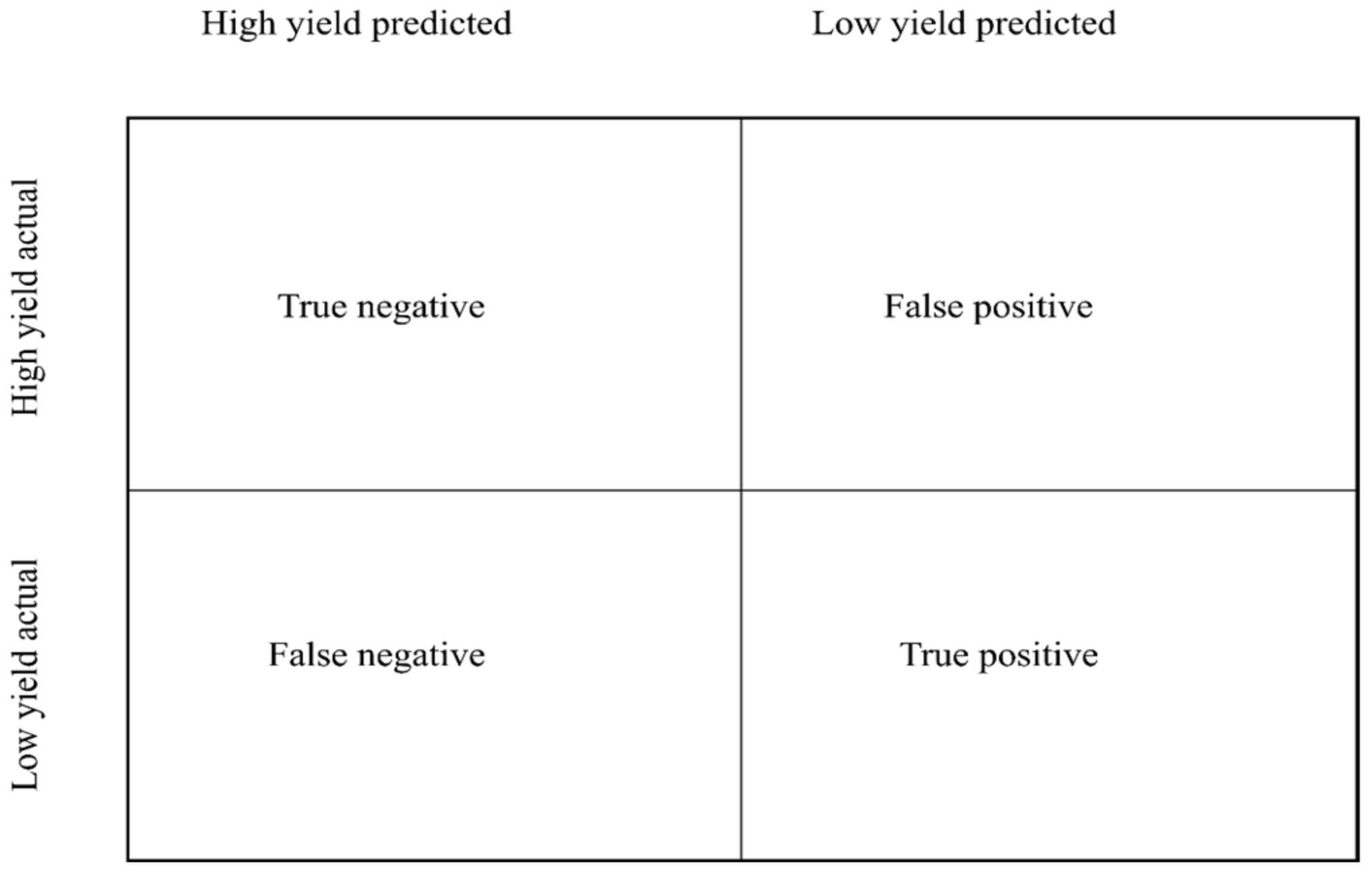
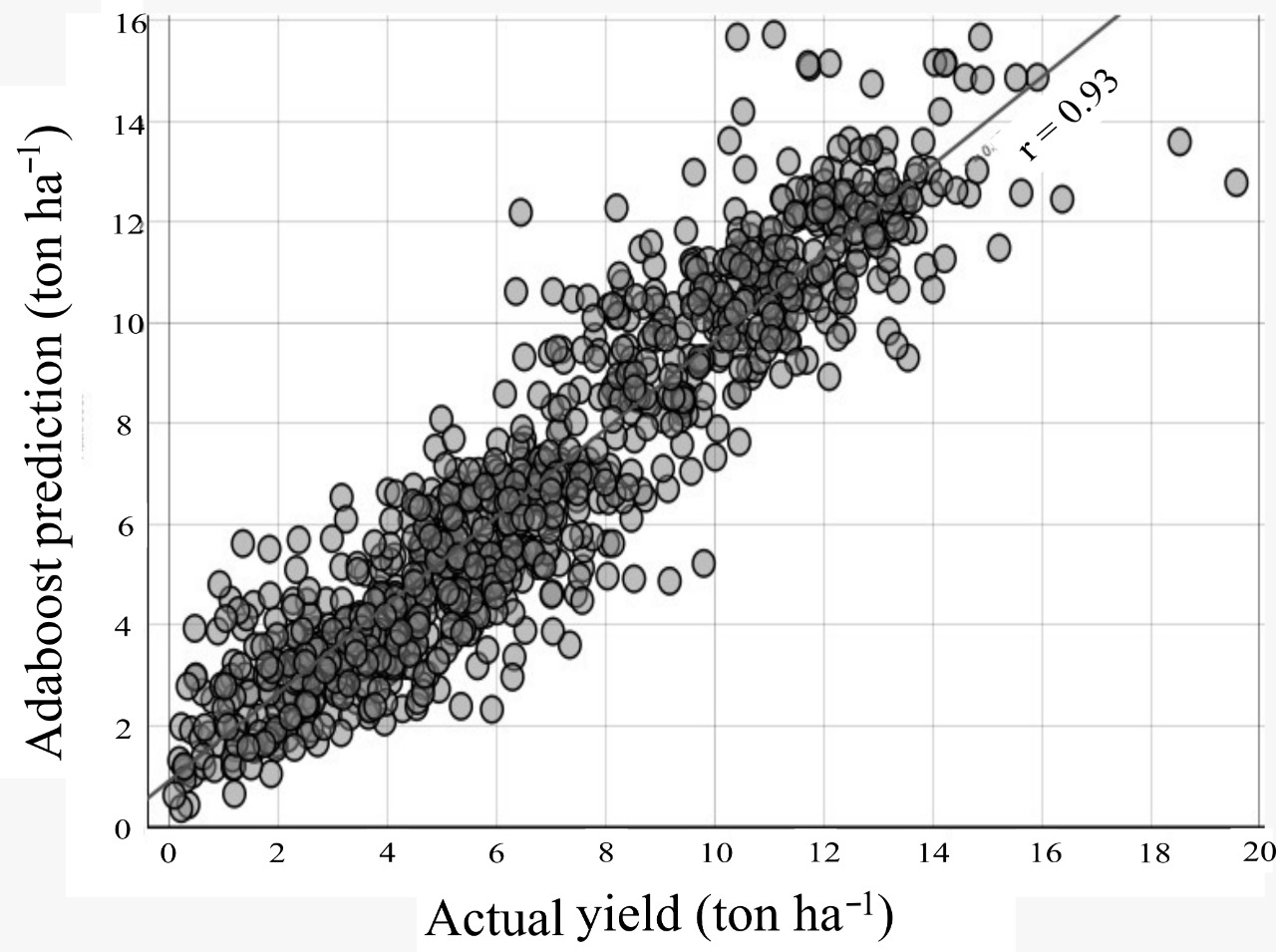
3.1. Model Accuracy
3.2. Random Forest Yield Prediction for Observational Data in 2018–2019
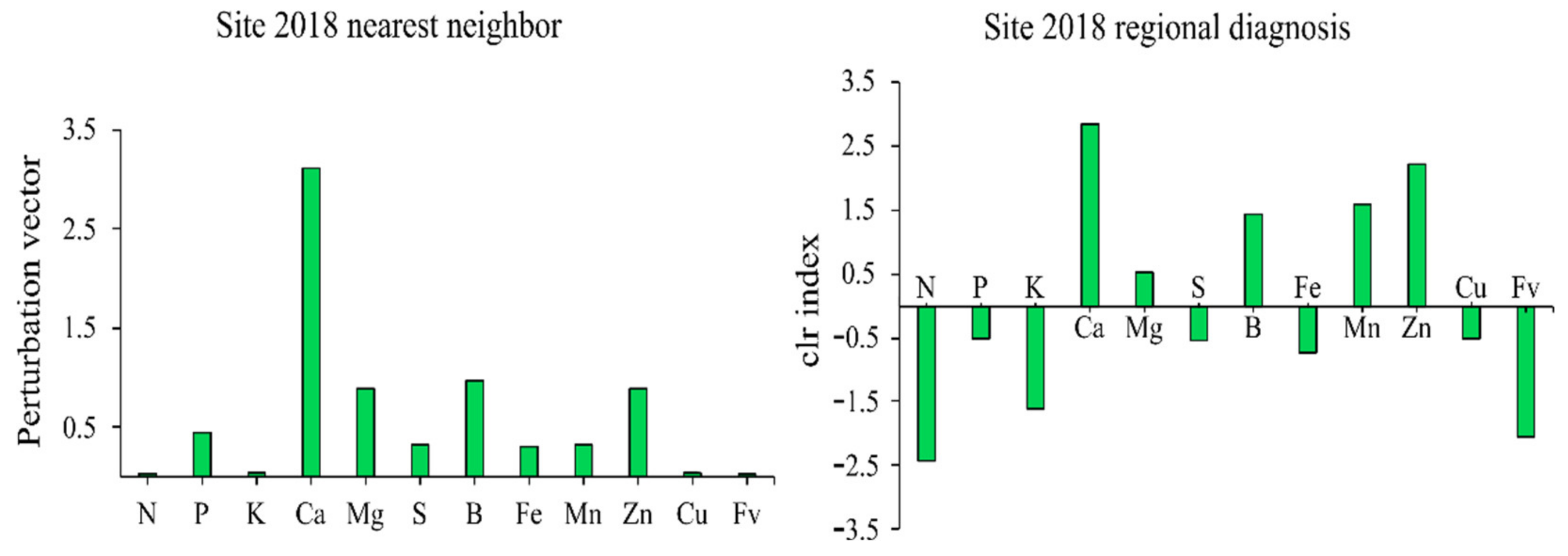
3.3. The False Positive Specimens at Site in 2018
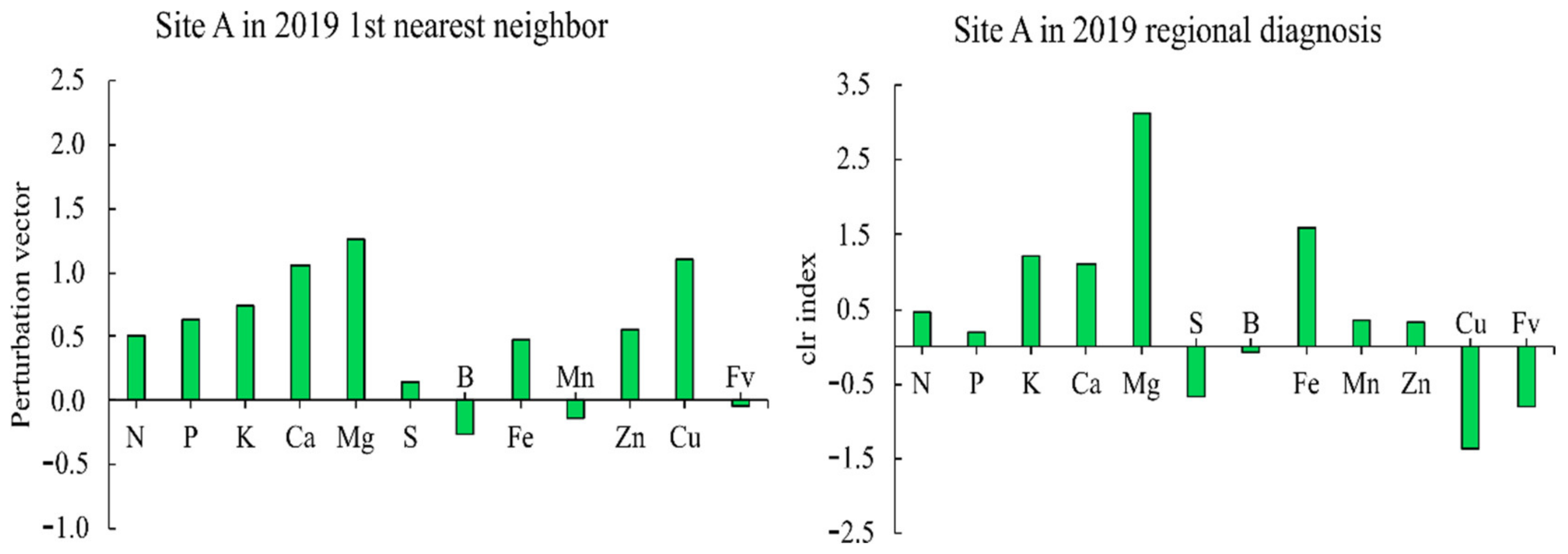
3.4. The True Positive Specimens at Site A in 2019
4. Discussion
4.1. Factor-Specific Optimum Nutrient Levels
4.2. Prediction of Garlic Yields and Nutrient Limitations
4.3. Need for Large and Diversified Datasets
5. Conclusions
Supplementary Materials
Author Contributions
Funding
Institutional Review Board Statement
Informed Consent Statement
Data Availability Statement
Acknowledgments
Conflicts of Interest
References
- Cunha, M.L.P.; Oliveira, T.F.; Clemente, J.M.; Gentil, T.G.; de Aquino, L.A. Modeling of nutrients demands in garlic crop. Aust. J. Crop Sci. 2015, 9, 1205–1213. [Google Scholar] [CrossRef]
- Cunha, M.L.P.; Aquino, L.A.; Novais, R.F.; Clemente, J.M.; de Aquino, P.M.; Oliveira, T.F. Diagnosis of the Nutritional Status of Garlic Crops. Rev. Bras. Ciência Solo 2016, 40, e0140771. [Google Scholar] [CrossRef]
- Martínez-López, J.A.; López-Urrea, R.; Martínez-Romero, Á.; Pardo, J.J.; Montoya, F.; Domínguez, A. Improving the Sustainability and Profitability of Oat and Garlic Crops in a Mediterranean Agro-Ecosystem under Water-Scarce Conditions. Agronomy 2022, 12, 1950. [Google Scholar] [CrossRef]
- Sánchez-Virosta, Á.; Sánchez-Gómez, D. Thermography as a Tool to Assess Inter-Cultivar Variability in Garlic Performance along Variations of Soil Water Availability. Remote Sens. 2020, 12, 2990. [Google Scholar] [CrossRef]
- Moretti, C.L.; Berg, F.L.N.; Mattos, L.M.; Santos, J.Z.; Saminêz, T.C.O.; Resende, F.V.; Mendonça, J.L.; Lima, D.B. Chemical composition and physical properties of organically grown onions in central Brazil. Acta Hortic. 2005, 688, 317–321. [Google Scholar] [CrossRef]
- Buso, G.S.C.; Paiva, M.R.; Torres, A.C.; Resende, F.V.; Ferreira, M.A.; Buso, J.A.; Dusi, A.N. Genetic diversity studies of Brazilian garlic cultivars and quality control of garlic-clover production. Genet. Mol. Res. 2008, 7, 534–541. [Google Scholar] [CrossRef]
- De Resende, J.T.V.; Morales, R.G.F.; Zanin, D.S.; Resende, F.V.; de Paula, J.T.; Dias, D.M.; Galvão, A.G. Caracterização morfológica, produtividade e rendimento comercial de cultivares de alho. Hortic. Bras. 2013, 31, 157–162. [Google Scholar] [CrossRef]
- Inglis, P.W.; Mello, S.C.M.; Martins, I.; Silva, J.B.T.; Macêdo, K.; Sifuentes, D.N.; Valadares-Inglis, M.C. Trichoderma from Brazilian garlic and onion crop soils and description of two new species: Trichoderma azevedoi and Trichoderma peberdyi. PLoS ONE 2020, 15, e0228485. [Google Scholar] [CrossRef]
- Amorim, J.R.D.A.; Fernandes, P.D.; Gheyi, H.R.; Azevedo, N.C.D. Efeito da salinidade e modo de aplicação da água de irrigação no crescimento e produção de alho. Pesqui. Agropecuária Bras. 2002, 37, 167–176. [Google Scholar] [CrossRef][Green Version]
- Hahn, L.; Paviani, A.C.; Feltrim, A.L.; Wamser, A.F.; Rozane, D.E.; Reis, A.R. dos Nitrogen doses and nutritional diagnosis of virus-free garlic. Rev. Bras. Ciência Solo 2020, 44, e0190067. [Google Scholar] [CrossRef]
- Hoogerheide, E.S.S.; Azevedo Filho, J.A.; Vencovsky, R.; Zucchi, M.I.; Zago, B.W.; Pinheiro, J.B. Genetic variability of garlic accessions as revealed by agro-morphological traits evaluated under different environments. Genet. Mol. Res. 2017, 16, gmr16029612. [Google Scholar] [CrossRef]
- Jones, J.B.; Case, V.W. Sampling, Handling, and Analyzing Plant Tissue Samples. In Soil Testing and Plant Analysis; SSSA Book Series; John Wiley & Sons, Ltd.: Madison, WI, USA, 1990; pp. 549–562. ISBN 9780891188629. [Google Scholar]
- Peck, T.R. Soil testing: Past, present and future. Commun. Soil Sci. Plant Anal. 1990, 21, 1165–1186. [Google Scholar] [CrossRef]
- Ruel, J.C.; Horvath, R.; Ung, C.H.; Munson, A. Comparing height growth and biomass production of black spruce trees in logged and burned stands. For. Ecol. Manag. 2004, 193, 371–384. [Google Scholar] [CrossRef]
- Munson, R.D.; Nelson, W.L. Principles and Practices in Plant Analysis. In Soil Testing and Plant Analysis; Westerman, R., Ed.; SSSA Book Series; John Wiley & Sons, Ltd.: Madison, WI, USA, 1990; pp. 359–387. ISBN 9780891188629. [Google Scholar]
- Wilkinson, S.R.; Grunes, D.L.; Sumner, M.E. Nutrient Interactions in Soil and Plant Nutrition. In Handbook of Soil Science; Routledge: Boca Raton, FL, USA, 2000; pp. 89–112. [Google Scholar]
- Walworth, J.L.; Sumner, M.E. The Diagnosis and Recommendation Integrated System (DRIS). In Advances in Soil Science; Springer: Berlin/Heidelberg, Germany, 1987; pp. 149–188. [Google Scholar]
- Leitzke Betemps, D.; Vahl de Paula, B.; Parent, S.-É.; Galarça, S.P.; Mayer, N.A.; Marodin, G.A.B.; Rozane, D.E.; Natale, W.; Melo, G.W.B.; Parent, L.E.; et al. Humboldtian Diagnosis of Peach Tree (Prunus persica) Nutrition Using Machine-Learning and Compositional Methods. Agronomy 2020, 10, 900. [Google Scholar] [CrossRef]
- De Lima Neto, A.J.; de Deus, J.A.L.; Rodrigues Filho, V.A.; Natale, W.; Parent, L.E. Nutrient Diagnosis of Fertigated “Prata” and “Cavendish” Banana (Musa spp.) at Plot-Scale. Plants 2020, 9, 1467. [Google Scholar] [CrossRef]
- Vahl de Paula, B.; Squizani Arruda, W.; Etienne Parent, L.; Frank de Araujo, E.; Brunetto, G. Nutrient Diagnosis of Eucalyptus at the Factor-Specific Level Using Machine Learning and Compositional Methods. Plants 2020, 9, 1049. [Google Scholar] [CrossRef]
- Lemaire, G.; Sinclair, T.; Sadras, V.; Bélanger, G. Allometric approach to crop nutrition and implications for crop diagnosis and phenotyping. A review. Agron. Sustain. Dev. 2019, 39, 27. [Google Scholar] [CrossRef]
- Jarrell, W.M.; Beverly, R.B. The Dilution Effect in Plant Nutrition Studies; Academic Press: Cambridge, MA, USA, 1981; Volume 34, pp. 197–224. ISBN 0065-2113. [Google Scholar]
- Keppel, G.; Kreft, H. Integration and synthesis of quantitative data: Alexander von Humboldt’s renewed relevance in modern biogeography and ecology. Front. Biogeogr. 2019, 11, 1–6. [Google Scholar] [CrossRef]
- Aitchison, J. The Statistical Analysis of Compositional Data; Chapman & Hall, Ltd.: London, UK, 1986; ISBN 0412280604. [Google Scholar]
- Aitchison, J. Principles of Compositional Data Analysis. Inst. Math. Stat. Lect. Notes Monogr. Ser. 1994, 24, 73–81. [Google Scholar] [CrossRef]
- Coulibali, Z.; Cambouris, A.N.; Parent, S.-É. Cultivar-specific nutritional status of potato (Solanum tuberosum L.) crops. PLoS ONE 2020, 15, e0230458. [Google Scholar] [CrossRef]
- Parent, S.-É. Why we should use balances and machine learning to diagnose ionomes. Authorea 2020, 1, 1–13. [Google Scholar] [CrossRef]
- Parent, S.-É.; Lafond, J.; Paré, M.C.; Parent, L.E.; Ziadi, N. Conditioning Machine Learning Models to Adjust Lowbush Blueberry Crop Management to the Local Agroecosystem. Plants 2020, 9, 1401. [Google Scholar] [CrossRef] [PubMed]
- Hahn, L.; Parent, L.-É.; Paviani, A.C.; Feltrim, A.L.; Wamser, A.F.; Rozane, D.E.; Ender, M.M.; Grando, D.L.; Moura-Bueno, J.M.; Brunetto, G. Garlic (Allium sativum) feature-specific nutrient dosage based on using machine learning models. PLoS ONE 2022, 17, e0268516. [Google Scholar] [CrossRef] [PubMed]
- Alvares, C.A.; Stape, J.L.; Sentelhas, P.C.; Gonçalves, J.L.M.; Sparovek, G. Köppen’s climate classification map for Brazil. Meteorol. Zeitschrift 2013, 22, 711. [Google Scholar] [CrossRef]
- United States Department of Agriculture. Soil Survey Staff Keys to Soil Taxonomy, 12th ed.; United States Department of Agriculture: Washington, DC, USA, 2014. [Google Scholar]
- Tedesco, M.J.; Gianello, C.; Bissani, C.A.; Bohnen, H.; Volkweiss, S.J. Análise de Solo, Plantas e Outros Materiais; Universidade Federal do Rio Grande do Sul: Porto Alegre, Brazil, 1995. [Google Scholar]
- Da Silva, F.C. Manual de Análises Químicas de Solos, Plantas e Fertilizantes; Embrapa Informação Tecnológica: Brasília, Brazil, 2009. [Google Scholar]
- Dos Santos, F.C.; Neves, J.C.L.; Novais, R.F.; Alvarez, V.V.H.; Sediyama, C.S. Modelagem da recomendação de corretivos e fertilizantes para a cultura da soja. Rev. Bras. Ciência Solo 2008, 32, 1661–1674. [Google Scholar] [CrossRef][Green Version]
- Murphy, J.; Riley, J.P. A modified single solution method for the determination of phosphate in natural waters. Anal. Chim. Acta 1962, 27, 31–36. [Google Scholar] [CrossRef]
- MclNTOSH, J.J.; COX, J.E. Colorimetric Determination of Boron in Porcelain Enamel Frits. J. Am. Ceram. Soc. 1960, 43, 123–124. [Google Scholar] [CrossRef]
- Luengo, R.F.A.; Calbo, A.G.; Lana, M.M.; Moretti, C.L.; Henz, G.P. Classificação de Hortaliças; Ministério da Agricultura, Pecuária e Abastecimento: Marília, Brazil, 1999; p. 63. [Google Scholar]
- Epagri. Empresa de Pesquisa Agropecuária e Extensão Rural de Santa. In Banco de Dados de Variáveis Ambientais de Santa Catarina; Epagri: Florianopolis, Brazil, 2020; ISBN 2674-9521. [Google Scholar]
- Agriculture and Agri-Food Canada. Government of Canada Cool Wave Days for Cool Season/Overwintering Crops (>5 °C); Agriculture and Agri-Food Canada: Ottawa, ON, Canada, 2018. [Google Scholar]
- Tremblay, N.; Bouroubi, Y.M.; Bélec, C.; Mullen, R.W.; Kitchen, N.R.; Thomason, W.E.; Ebelhar, S.; Mengel, D.B.; Raun, W.R.; Francis, D.D.; et al. Corn Response to Nitrogen is Influenced by Soil Texture and Weather. Agron. J. 2012, 104, 1658–1671. [Google Scholar] [CrossRef]
- Parent, L.E.; Dafir, M. A Theoretical Concept of Compositional Nutrient Diagnosis. J. Am. Soc. Hortic. Sci. 1992, 117, 239–242. [Google Scholar] [CrossRef]
- Rozane, D.E.; Vahl de Paula, B.; Wellington Bastos de Melo, G.; Haitzmann dos Santos, E.M.; Trentin, E.; Marchezan, C.; Stefanello da Silva, L.O.; Tassinari, A.; Dotto, L.; Nunes de Oliveira, F.; et al. Compositional Nutrient Diagnosis (CND) Applied to Grapevines Grown in Subtropical Climate Region. Horticulturae 2020, 6, 56. [Google Scholar] [CrossRef]
- Montañés, L.; Heras, L.; Abadía, J.; Sanz, M. Plant analysis interpretation based on a new index: Deviation from optimum percentage (DOP). J. Plant Nutr. 1993, 16, 1289–1308. [Google Scholar] [CrossRef]
- CQFS-RS/SC. Manual de Calagem e Adubação para os estados do Rio Grande so Sul e Santa Catarina; Sociedade Brasileira de Ciência do Solo/Núcleo Regional Sul, 11th ed.; Westphalen, F., Ed.; Sociedade Brasileira de Ciência do Solo: Viçosa, Brazil, 2016; ISBN 978-85-66301-80-9. [Google Scholar]
- Barber, S. Soil Nutrient Bioavailability. A Mechanistic Approach, 2nd ed.; Wiley: New York, NY, USA, 1995. [Google Scholar]
- Bray, R.H. Confirmation of the nutrient mobility concept of soil-plant relationships. Soil Sci. 1963, 95, 124–130. [Google Scholar] [CrossRef]
- Nowaki, R.H.D.; Parent, S.-É.; Cecílio Filho, A.B.; Rozane, D.E.; Meneses, N.B.; dos Santos da Silva, J.A.; Natale, W.; Parent, L.E. Phosphorus Over-Fertilization and Nutrient Misbalance of Irrigated Tomato Crops in Brazil. Front. Plant Sci. 2017, 8, 825. [Google Scholar] [CrossRef]
- Lemaire, G.; Salette, J.; Sigogne, M.; Terrasson, J.-P. Relation entre dynamique de croissance et dynamique de prélèvement d’azote pour un peuplement de graminées fourragères. I.—Etude de l’effet du milieu. Agronomie 1984, 4, 423–430. [Google Scholar] [CrossRef]
- Andrews, M.; Sprent, J.I.; Raven, J.A.; Eady, P.E. Relationships between shoot to root ratio, growth and leaf soluble protein concentration of Pisum sativum, Phaseolus vulgaris and Triticum aestivum under different nutrient deficiencies. Plant Cell Environ. 1999, 22, 949–958. [Google Scholar] [CrossRef]
- Bradshaw, A.D. Evolutionary Significance of Phenotypic Plasticity in Plants; Dunlap, J.C., Friedmann, T., Goodwin, S.F., Eds.; Academic Press: Cambridge, MA, USA, 1965; Volume 13, pp. 115–155. ISBN 0065-2660. [Google Scholar]
- Wit, C.T. de Resource use efficiency in agriculture. Agric. Syst. 1992, 40, 125–151. [Google Scholar] [CrossRef]
- Beaufils, E.R. Physiological diagnosis: A guide for improving maize production based on principles developed for rubber trees. Fertil. Soc. South Afr. J. 1971, 1, 1–28. [Google Scholar]
- Courbet, G.; Gallardo, K.; Vigani, G.; Brunel-Muguet, S.; Trouverie, J.; Salon, C.; Ourry, A. Disentangling the complexity and diversity of crosstalk between sulfur and other mineral nutrients in cultivated plants. J. Exp. Bot. 2019, 70, 4183–4196. [Google Scholar] [CrossRef]
- Jeanne, T.; Parent, S.-É.; Hogue, R. Using a soil bacterial species balance index to estimate potato crop productivity. PLoS ONE 2019, 14, e0214089. [Google Scholar] [CrossRef]


| Yield Classification | Predicted Yield | |
|---|---|---|
| Actual yield | High | Low |
| High | 135 TN | 40 FP |
| Low | 40 FN | 699 TP |
| Combination of Factors | Regression | Classification |
|---|---|---|
| R2 | Accuracy | |
| Tissue analysis | 0.750 | 0.891 |
| Tissue analysis, cultivar | 0.789 | 0.886 |
| Tissue analysis, cultivar, preceding crop | 0.791 | 0.894 |
| Tissue analysis, cultivar, preceding crop, fertilization | 0.820 | 0.898 |
| Tissue analysis, cultivar, preceding crop, fertilization, plantation date | 0.839 | 0.891 |
| Tissue analysis, cultivar, preceding crop, fertilization, plantation date, climatic indices | 0.840 | 0.907 |
| Tissue analysis, cultivar, preceding crop, fertilization, plantation date, climatic indices, soil test | 0.855 | 0.912 |
| Nutrient | 8 Mg ha−1 | 11 Mg ha−1 | t-Test | ||
|---|---|---|---|---|---|
| Mean | SD | Mean | SD | Probability | |
| N | 3.430 | 0.157 | 3.403 | 0.166 | 0.112 ns |
| P | 1.365 | 0.209 | 1.317 | 0.167 | 0.011 * |
| K | 3.255 | 0.235 | 3.364 | 0.193 | 0.000 ** |
| Ca | 1.463 | 0.345 | 1.642 | 0.242 | 0.000 ** |
| Mg | 0.679 | 0.229 | 0.532 | 0.123 | 0.000 ** |
| S | 1.843 | 0.423 | 1.938 | 0.379 | 0.019 * |
| Fe | −3.786 | 0.393 | −3.814 | 0.423 | 0.509 ns |
| Mn | −3.070 | 0.505 | −3.062 | 0.415 | 0.861 |
| Zn | −3.583 | 0.481 | −3.725 | 0.395 | 0.001 ** |
| Cu | −3.918 | 0.336 | −3.877 | 0.280 | 0.186 ns |
| B | −4.516 | 0.828 | −4.495 | 1.012 | 0.836 ns |
| Fv | 6.838 | 0.191 | 6.779 | 0.186 | 0.002 ** |
| Number | n = 344 | n = 128 | - | ||
| Feature ‡ | Site 2018 | Site 2019 A | Site 2019 B | True Negative Specimens |
|---|---|---|---|---|
| N | 20.0–33.3 | 33.6–39.2 | 19.6–36.4 | 23.1–45.5 |
| P | 4.8–6.6 | 4.5–5.0 | 3.6–6.9 | 2.1–5.8 |
| K | 28.4–81.2 | 41.9–52.0 | 10.8–29.9 | 12.7–54.5 |
| Ca | 15.7–50.4 | 7.1–9.7 | 3.4–5.1 | 0.9–9.8 |
| Mg | 2.9–7.9 | 3.9–5.1 | 1.7–8.5 | 0.8–2.5 |
| S | 6.5–9.4 | 3.9–5.8 | 3.3–7.0 | 3.5–14.5 |
| B | 54–86 | 18–23 | 26–40 | 0.9–44 |
| Fe | 32–197 | 98–339 | 28–137 | 13–515 |
| Mn | 59–176 | 35–92 | 19–39 | 11–115 |
| Zn | 43–107 | 26–38 | 22–57 | 10–154 |
| Cu | 16–54 | 4–8 | 7–56 | 3–219 |
| Degree-days (>5 °C) | 461 | 582 | 347 | 297–421 |
| Rainfall (mm) | 172 | 41 | 35 | 104–241 |
| SDI | 0.57 | 0.10 | 0.04 | 0.54–0.64 |
| Variable | Unit | Diagnosed | First Nearest | Second Nearest | Third Nearest |
|---|---|---|---|---|---|
| Yield | Mg ha−1 | 15.5 | 11.2 | 11.0 | 11.1 |
| Tissue | |||||
| N | g kg−1 | 29.5 | 30.0 | 28.9 | 28.0 |
| P | g kg−1 | 5.9 | 4.1 | 3.2 | 2.8 |
| K | g kg−1 | 35.0 | 33.3 | 30.8 | 32.0 |
| Ca | g kg−1 | 21.0 | 5.1 | 4.4 | 4.8 |
| Mg | g kg−1 | 3.5 | 1.8 | 1.9 | 1.7 |
| S | g kg−1 | 7.6 | 5.8 | 4.7 | 8.3 |
| B | mg kg−1 | 64 | 33 | 31 | 28 |
| Fe | mg kg−1 | 55 | 42 | 41 | 30 |
| Mn | mg kg−1 | 97 | 73 | 84 | 22 |
| Zn | mg kg−1 | 62 | 32 | 31 | 28 |
| Cu | mg kg−1 | 28 | 29 | 4 | 6 |
| Soil | |||||
| pHwater | - | 6.4 | 6.3 | 6.0 | 6.1 |
| Clay | % | 40 | 61 | 61 | 49 |
| OM | % | 5.7 | 3.6 | 3.8 | 3.2 |
| P | mg dm−3 | 131.2 | 8.6 | 8.9 | 19.4 |
| K | mg dm−3 | 400 | 298.1 | 552 | 132 |
| Ca | cmolc dm−3 | 12.4 | 8.5 | 7.1 | 9.4 |
| Mg | cmolc dm−3 | 4.9 | 2.3 | 3.1 | 3.7 |
| Treatment | |||||
| N | kg N ha−1 | 160 | 400 | 400 | 400 |
| P | kg P2O5 ha−1 | 680 | 0 | 400 | 100 |
| K | kg K2O ha−1 | 457 | 400 | 500 | 400 |
| Variable | Unit | Diagnosed | First Nearest | Second Nearest | Third Nearest |
|---|---|---|---|---|---|
| Yield | ton ha−1 | 9.7 | 13.9 | 11.0 | 11.4 |
| Tissue | |||||
| N | g kg−1 | 39.2 | 26.0 | 28.9 | 28.8 |
| P | g kg−1 | 4.8 | 2.9 | 3.2 | 2.6 |
| K | g kg−1 | 48.7 | 28.1 | 30.8 | 25.1 |
| Ca | g kg−1 | 8.4 | 4.1 | 4.4 | 3.6 |
| Mg | g kg−1 | 4.5 | 2.0 | 1.9 | 1.4 |
| S | g kg−1 | 5.1 | 4.5 | 4.7 | 7.9 |
| B | mg kg−1 | 202 | 272 | 315 | 255 |
| Fe | mg kg−1 | 1264 | 857 | 410 | 420 |
| Mn | mg kg−1 | 478 | 550 | 840 | 216 |
| Zn | mg kg−1 | 288 | 185 | 308 | 263 |
| Cu | mg kg−1 | 63 | 30 | 43 | 38 |
| Soil | |||||
| pHwater | 6.0 | 6.0 | 6.0 | 6.1 | |
| Clay | % | 39 | 61 | 61 | 49 |
| OM | % | 4.5 | 3.8 | 3.8 | 3.2 |
| P | mg dm−3 | 47.5 | 31.7 | 8.9 | 15.2 |
| K | mg dm−3 | 296 | 112.3 | 552 | 132 |
| Ca | cmolc dm−3 | 15.3 | 7.1 | 7.1 | 9.4 |
| Mg | cmolc dm−3 | 5.0 | 3.1 | 3.1 | 3.7 |
| Treatment | |||||
| N | kg N ha−1 | 130 | 300 | 300 | 300 |
| P | kg P2O5 ha−1 | 300 | 800 | 400 | 0 |
| K | kg K2O ha−1 | 150 | 400 | 500 | 400 |
Publisher’s Note: MDPI stays neutral with regard to jurisdictional claims in published maps and institutional affiliations. |
© 2022 by the authors. Licensee MDPI, Basel, Switzerland. This article is an open access article distributed under the terms and conditions of the Creative Commons Attribution (CC BY) license (https://creativecommons.org/licenses/by/4.0/).
Share and Cite
Hahn, L.; Parent, L.-É.; Feltrim, A.L.; Rozane, D.E.; Ender, M.M.; Tassinari, A.; Krug, A.V.; Berghetti, Á.L.P.; Brunetto, G. Local Factors Impact Accuracy of Garlic Tissue Test Diagnosis. Agronomy 2022, 12, 2714. https://doi.org/10.3390/agronomy12112714
Hahn L, Parent L-É, Feltrim AL, Rozane DE, Ender MM, Tassinari A, Krug AV, Berghetti ÁLP, Brunetto G. Local Factors Impact Accuracy of Garlic Tissue Test Diagnosis. Agronomy. 2022; 12(11):2714. https://doi.org/10.3390/agronomy12112714
Chicago/Turabian StyleHahn, Leandro, Léon-Étienne Parent, Anderson Luiz Feltrim, Danilo Eduardo Rozane, Marcos Matos Ender, Adriele Tassinari, Amanda Veridiana Krug, Álvaro Luís Pasquetti Berghetti, and Gustavo Brunetto. 2022. "Local Factors Impact Accuracy of Garlic Tissue Test Diagnosis" Agronomy 12, no. 11: 2714. https://doi.org/10.3390/agronomy12112714
APA StyleHahn, L., Parent, L.-É., Feltrim, A. L., Rozane, D. E., Ender, M. M., Tassinari, A., Krug, A. V., Berghetti, Á. L. P., & Brunetto, G. (2022). Local Factors Impact Accuracy of Garlic Tissue Test Diagnosis. Agronomy, 12(11), 2714. https://doi.org/10.3390/agronomy12112714