Precision Variable-Rate Spraying Robot by Using Single 3D LIDAR in Orchards

Abstract

Automatic navigation (AN) is an essential component to ensure the safety of pesticide application in orchards, whereas precision variable-rate spraying (PVS) serves as an indispensable technology for reducing the application of pesticides and protecting the environment. At present, AN and PVS are not closely combined. In this case, a single three-dimension (3D) light detection and ranging (LIDAR) sensor is hereby adopted to sense the information of fruit trees around the robot and determine the region of interest (ROI). Moreover, two-dimensional (2D) processing is conducted over the point clouds within the ROI to obtain the center-of-mass coordinates of fruit trees, and determine the vertical distance of the robot to the center line of the fruit tree row (FTR) based on the FTR on both sides using the Random Sample Consensus (RANSAC) algorithm. Then, the robot is controlled to drive along the center line of the FTR. At the same time, the speed and position of the robot are determined by the encoder and inertial measurement unit (IMU), and the IMU corrects the information collected from the zoned canopy of the fruit trees. The results present a lateral deviation (LD) of less than 22 cm and a course deviation (CD) of less than 4.02° during AN. Compared with the traditional spraying (TS), the PVS applies 32.46%, 44.34% and 58.14% less pesticide application, air drift and ground loss, respectively. With the spraying effect guaranteed, the single 3D LIDAR, the encoder and IMU realize the AN and PVS of the robot, reduce the volume of pesticide application, ground loss and air drift, and effectively control the pollution caused by pesticides to the environment.

1. Introduction

Plant protection in Chinese orchards accounts for about 40% of the total orchard management, with a significant workload of 6–10 applications required during a growth cycle [1]. TS with fixed parameters are generally used for the orchard plant protection operation, and the application of fixed spraying parameters results in too little pesticide application on some canopies and too much spraying on some canopies [2]. Chinese plant protection products (PPPs) are mostly driven manually, but more than half of them do not have cabs. Even when they do have cabs, the protection measures are simple and the operators are exposed to the application environment, making the operators easily poisoned [1,2].

The remote-controlled PPPs currently produced in China for orchards provide a degree of separation between operators and pesticides. However, the limited range of the remote-controlled PPPs does not completely separate people from the pesticides, and risks remain. It is why the complete separation of human and pesticides on PPPs is a prerequisite for operator safety [3].

Modern agricultural equipment is being developed in the direction of automation, information technology and intelligence, which will further promote the upgrading and iteration of the agricultural industry [4]. As the number of people working in Chinese agriculture decreases and the cost of labor increases, smart equipment, including navigation robots, is beginning to be used on a large scale in Chinese agriculture. Compared with other complex agricultural environments, modern orchards are planted in wide rows with narrow plant spacing, and the close connection between branch and leaf plants in a “tree wall” structure provides a simpler navigation environment.

The PPPs with AN function is completely separated from the pesticides, thereby guaranteeing the safety of the personnel during operation and improving the operation efficiency, which will occupy a large market in the PPPs. AN solution based on global navigation satellite systems (GNSS) have been completely applied to field operation environments [5,6]. However, Li et al. pointed out that GNSS positioning methods are not suitable for AN operation in orchard scenarios due to the loss of navigation satellite signals caused by the shading of fruit trees [7].

Current orchards AN operation relies on visual navigation and laser navigation [8]. Radcliffe et al. collected environmental information from the orchards using a multispectral camera and processed the canopy and sky information to identify the navigation line using a machine learning algorithm [9] (not specified in the paper, the navigation line refers to the center line of the FTR). Although vision sensors are provided with the advantages of low cost and rich information, the imaging quality is still easily disturbed by light and fails to directly obtain the depth information [8,10].

Laser navigation senses the orchard environment in real-time and obtains different fruit tree positions to achieve relative positioning of the robot using LIDAR. LIDAR has the advantages of active luminescence, high-range accuracy, and strong adaptability to the environment for all-weather operation. LIDAR can be classified into single-line 2D LIDAR and multi-line 3D LIDAR [11,12,13]. Based on the Simultaneous Localization and Mapping (SLAM) technology, Santos et al. also developed the GNSS-independent VineSlam localization and mapping method and the vineyard-specific path planner “AgRobPP”, which are proven in mapping and path planning and can perform tasks such as automatic charging [14]. The SLAM technology based on 3D LIDAR can detect the 3D information of the surrounding environment and enhance the safety of the moving robot [15]. However, it increases the computational burden and demands higher computational performance. Liu et al. extracted navigation lines and AN operations using 3D LIDAR, but did not obtain the external features (canopy volume and leaf area index (LAI), etc.) of fruit trees [13]. The above studies achieved AN operations using 2D LIDAR or the 2D processing of 3D LIDAR, discarding the 3D information of the robot’s surroundings.

Vision sensors and LIDAR in AN operation can be used for collecting information on the external features of the canopy of fruit trees in orchards [2,16], among which, LIDAR presents unique and excellent performance and is most widely used in orchards PVS [16,17,18,19,20]. In this case, it can be used not only for AN, but also for acquiring information of surrounding fruit trees for PVS. However, the use of LIDAR to obtain the LAI of fruit tree canopies requires a large number of point clouds [21,22], and the calculation method is too complicated to realize real-time online calculation [22,23]. The fruit tree canopy features should be calculated in real time to control the spray volume during PVS operation, but considerable studies have proven the existence of a strong linear relationship between the LAI and the fruit tree canopy volume during the same growth period of fruit trees [21,24,25,26,27]. In this case, the LAI can be replaced by the fruit tree canopy volume (FTCV) in the case of a certain growth cycle of fruit trees.

The combination of pulse width modulation (PWM) technology with PVS according to the FTCV has changed the traditional spraying operation with continuous spraying without regard to target differences, achieving the purpose of saving pesticide application, reducing air drift and ground loss, improving the efficiency of spraying operation, which is also endowed with the advantages of low computational intensity and high reliability [26,27]. Liu et al. achieved the calculation of canopy volume of fruit trees by a simple sensor array composed of ultrasonic sensors and laser sensors, and the calculation accuracy reached more than 88% [16], indicating that simple sensors can achieve high accuracy of canopy volume measurement, whereas 3D LIDAR measures more data and fully meets the high accuracy of canopy volume measurement. A vertically mounted LIDAR was adopted by both Li et al. [28] and Xue et al. [27] to obtain the external characteristics of fruit trees for PVS and achieve the purpose of saving pesticides and reducing air drift and ground loss. Manned vehicles are used by most of the above PVS devices for application, and are exposed to the risk of pesticide poisoning to the operator increased [10,25].

In the above study, the LIDAR was horizontally mounted during AN operation to obtain as much surrounding information as possible, but was mounted vertically to obtain as many fruit tree external features as possible for PVS, failing to enable AN operation [13]. Compared with the 2D LIDAR, the horizontally mounted 3D LIDAR can detect the 3D information of the surrounding environment. For the above situation, the horizontally mounted 3D LIDAR is used to change the ROI range and calculate the canopy volume of zoned fruit trees, and finally achieve AN and PVS, thus providing a new solution for AN and PVS in orchards. 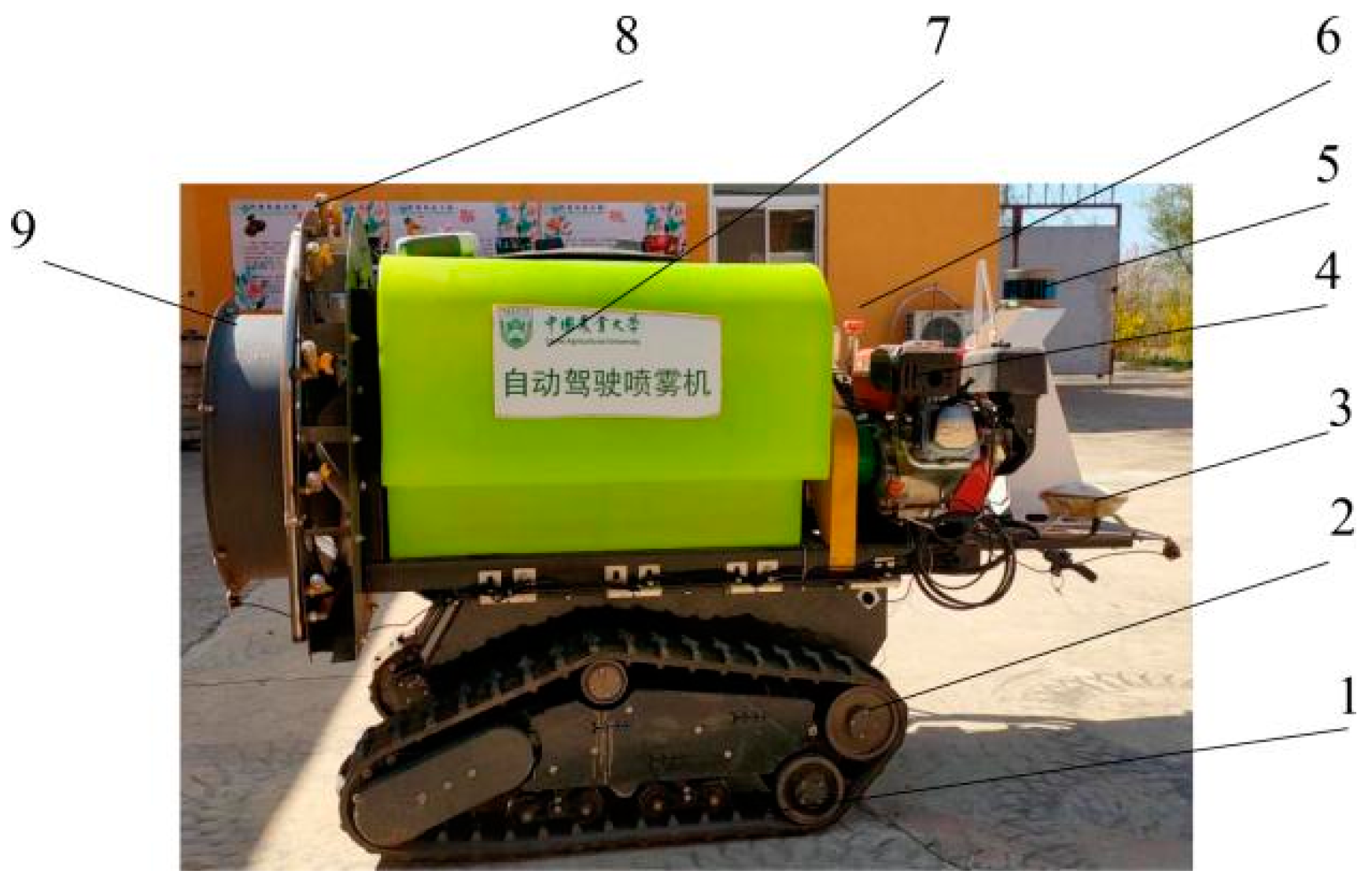The remaining part of this paper is organized as follows: Section 2 introduces the electronic hardware system, walking system, spraying system, AN test system and adjustment of the spraying system of the precision variable-rate spraying robot (PVSR); Section 3 proposes the algorithm to realize the travel along the center line of the FTR, and also the zoned canopy volume calculation and PVS decision based on the point cloud data collected within the ROI; Section 4 is further designed to verify the performance of AN and PVS, in which the LD and CD of the PVSR are tested by RTK GNSS at normal spraying speed, whereas the volume of droplet deposit (DD), ground loss and air drift of the orchard sprayer are tested by the internationally established DD and air drift standards. A comparison is correspondingly made with TS, automatic targeting spraying (ATS) and PVS; Section 5 presents the analysis and discussion of the test results; Section 6 offers the conclusion.

2. Hardware Design

2.1. PVSR Composition

The hereby designed PVSR (designed by authors, produced by AGILE.X Inc., Shenzhen, Guangdong, China), with dimensions of 1.5 m × 1.5 m × 1.4 m in length, width and height, respectively, and a maximum capacity of 300 L, is shown in Figure 1. This PVSR mainly consists of an electronic hardware system, a walking system, a spraying system and an AN test system. Electronic products with poor waterproof capability such as industrial personal computer (IPC) and IMU are installed in the chassis at the bottom of the tank to prevent irreversible damage caused by the droplets entering it during the operation.

2.2. Electronic Hardware System

As shown in Figure 2, the electronic hardware system is integrated, which can sense the surrounding environment in real-time, obtain information about the body, make decisions, and execute them concretely. It is divided into sensor module, control module, driver module, PVS module and power module in accordance with the functions. The green line in Figure 2 indicates the power supply, whereas the yellow colored lines represent the information transmission. Only the STM32 microcontroller unit (MCU) and IPC communicate in both directions.

2.2.1. Sensor Module

The sensor module mainly consists of 3D LIDAR (RoboSense Inc., Shenzhen, Guangdong, China), E6B2-CWZ6C encoder (Omron Inc., Hyuga, Kyoto, Japan) and IMU (Hongye Inc., Shenzhen, Guangdong, China), etc. LIDAR senses the surroundings of the PVSR and provides data support for AN and PVS. The 16-wire mechanical LIDAR can uninterruptedly scan the surrounding fruit trees at 360° horizontally and 30° vertically (15° above and below the LIDAR level), and provide up to 320,000 data points per second, with a maximum detection distance of 150 m, a detection accuracy of ±2 cm, and a vertical angle resolution of 2°. The horizontal angle resolution is 0.09°, 0.18° and 0.38° while working at 5 Hz, 10 Hz and 20 Hz, respectively (10 Hz is hereby adopted), with DC 12V power supply and 100M Ethernet communication with the IPC.

The encoder acquires the vehicle speed information, whereas the IMU acquires the PVSR course angle and position information. The encoder with a resolution of 1000 P/R (pulse/ring), is co-axially connected to the active wheel (diameter 24 cm) of the PVSR via a connecting shaft. The IMU is an ICM-20948 IMU, with a Kalman filter program, and provides stable and accurate data. The static accuracy is 0.05°/s; the dynamic accuracy is 0.1°/s in X and Y directions; the Z-axis accuracy is 1°/s without magnetic field interference; the acceleration accuracy is 0.02 g; the gyroscope accuracy is 0.06°/s; and the maximum data output frequency is 200 Hz (100 Hz is hereby adopted).

2.2.2. Control Module

With a data volume of 320,000 points cloud per second, the central processing unit (CPU, Intel Inc., Portland, OR, USA) must be extremely powerful. For this reason, we chose a Chinese IPC equipped with an i7 10510U processor, 16G of RAM, 1T of SSD, Ubuntu 18.04 Linux pre-installed, RS232, Ethernet, USB, and RS485 communication interfaces, and a 9–36V DC power supply. This study requires MCU to control the motor and solenoid valve, the MCU also takes the speed information and uploads it to the IPC. In this paper, the M3S type STM32 MCU (QiXingChong Inc., Dongguan, Guangdong, China) is hereby selected, which has a chip of stm32f103zet6, cortex-M3 protocol, 144 pins, 512 k flash memory, 72 MHz main frequency, and multiple communication interfaces such as CAN, USB and RS232. The classical proportional-integral-derivative (PID) algorithm is used to control the motor rotation through the motor driver and realize the precise motion of the PVSR.

2.2.3. Drive Module

The implementation of AN and PVS requires not only hardware for sensing, processing and transmitting information, but also specific drive components. In this study, two 800 W brushless servomotors (SDGA08C11AB, Xunkong Inc., Jiaxing, Zhejiang, China, 48 V power supply) with a 1:30 gearbox (60TDF-147050-L2H, Xunkong Inc., Jiaxing, Zhejiang, China) were selected to power the PVSR, along with a SDGA-21A servo driver, which accepts the control angular speed signals from the MCU via CAN bus (communication speed 500 k bit per second (bps), Intel coding format).

2.2.4. PVS Module

The PVS actuator consists of a 2P025-08 solenoid valve (24 V supply power, AIRTAC Inc., Ningbo, Zhejiang, China) that controls the on/off function of the pipe and an N-channel field effect N-Metal-Oxide-Semiconductor (NMOS) tube that controls the on/off function of the solenoid valve power supply. The NMOS tube is controlled by a high or low-level output from the IO port of the MCU.

2.2.5. Power Module

In addition to the functional modules mentioned above, a power module is required to provide the power supply for each module. In this case, a 48 V lithium iron phosphate battery (SK-48V100Ah, Jisheng Inc., Shenzhen, Guangdong, China) with a battery capacity of 100 Ah and a full charge voltage of about 55.2 V is selected. A voltage regulation module and a power display module are built-in, which can continuously supply power for 3–5 h under normal conditions and make automatic alarms when the voltage is lower than 47.5 V using a buzzer. It takes about 6 h to be fully charged. At the same time, there are voltage regulators installed to provide stable voltage for different functional modules (5, 12, 24 and 48 V power supply).

2.3. Walking System

The active wheels drive the rubber tracks that move the robot forward, the five loading wheels support the body weight, and three guiding wheels are used to guide and support the tracks and adjust the tightness of the tracks. The PVSR achieves differential steering and 360° in situ steering by means of different speeds of the left and right active wheels. The spring suspension was designed to give the PVSR high ground clearance and good ground adaptation. When unloading, the maximum moving speed of PVSR is 1.5 m/s, the maximum climbing angle is 30°, and the minimum distance between the frame and the ground is 250 mm, which allows it to move flexibly in the orchard.

2.4. Spraying System

The spraying system is made up of a gasoline engine (Yamaha Inc. Maebashi, Gunma, Japan), piston pump (Liannong Inc., Taizhou, Zhejiang, China), drive shaft, axial fan (Huinong Inc., Weifang, Shandong, China), liquid pipeline, pressure regulation valve (Yifeng Inc., Jinhua, Zhejiang, China), tank, solenoid valve, full cone nozzles, and fan deflectors. The robot uses air-assisted spraying technology. A 26A piston pump is adopted to provide liquid pressure and adjust the pressure of the whole spraying system through the pressure regulation valve and keep the pressure stable during the spraying operation. The piston pump is driven by a V-belt on the output shaft of the 170 F gasoline engine. The axial fan at the rear of the body is connected by a drive shaft to a pulley at the front of the body, which is also driven by the 170 F gasoline engine. The liquid from the tank enters the three-way liquid distributor via the piston pump to the Disc-Core type full cone nozzle (D3 DC31 type, TeeJet Inc., Wheaton, IL, USA, flow rate about 1.45 L/min at 5 bar) [29], with a solenoid valve installed between the nozzle and the liquid pipeline. Each nozzle is controlled by a solenoid valve and the spray angle of the nozzle is 63°. Travel speed is 1.25 m/s when the PVSR is spraying.

2.5. AN Test System

In order to verify the AN performance of the PVSR, the mobile trajectory measurement system needs to have a high accuracy so that it can be directly used as the reference true value. The “P3-DU” RTK GNSS positioning system (Huazheng Inc. Beijing, China) is compatible with GLONASS, Galileo, QZSS, SBAS, BDS, and GPS, is hereby adopted. The positioning system incorporates real-time differential algorithms to provide centimeter positioning accuracy, ±1 cm horizontal positioning accuracy, initialization time <10 s, data output frequency up to 20 Hz (20 Hz is used), and a power supply range of 9 to 36 V DC. The RTK GNSS mobile station (±2 cm movement accuracy) on the robot has a linear distance of 0.5 m from the center of the body and a vertical distance of 0.4 m.

2.6. Adjusting the Nozzles and Fan Deflectors

There are 10 nozzles and 8 fan deflectors symmetrically distributed on both sides of the PVSR, as shown in Figure 3. The nozzles and deflectors are arranged counter-clockwise from left to right: nozzle 1–nozzle 10 and deflector 1–deflector 8. The nozzles on either side of the robot are set to align with the fruit tree canopy (FTC), whereas deflector 1 and deflector 8, deflector 4 and deflector 5 are connected to each other to prevent airflow overflow, and the remaining deflectors form six air outlets corresponding to the upper, middle and lower of the fruit tree on both sides. The adjustment is complete when the direction of the ribbon float mounted on deflectors 1, 4, 5 and 8 is aligned with the overall FTC after the axial fan has started. The air velocity at each outlet is approximately 20 m/s (from 15 m/s to 23 m/s) at each outlet. The adjusted height from the ground and the angle to the ground of the nozzle and the deflector are shown in

Table 1. Nozzles and fan deflectors’ position.

Type	Position	Number
		1	2	3	4	5
Nozzles	Angle/°	15	25	40	55	72
	Height/cm	60	76	90	105	119
Deflectors	Angle/°	10	29.5	47.5	70	70
	Height/cm	52.5	82.5	101	114.5	114.5

.

3. Implementation Principles and Software Design

A reasonable workflow should be designed, and related programs should be written to realize the functions of the PVSR, as shown in the flow chart of Figure 4. The specific display process will be expanded and described as follows.

3.1. Construction of the Robot Motion Kinematic Model

The world coordinate system (WCS) is constructed by taking the center line of FTR at the starting position as the origin and the center line of FTR as the X-axis. The forward direction of the PVSR is the X-positive direction, whereas the left side of the PVSR is the Y-positive direction. As shown in Figure 5, the body coordinate system (BCS) is constructed with the center point (O_R) of the PVSR as the origin of the BCS. Considering the adoption of differential steering of the left and right wheels, the instantaneous velocity ($V_c$, m/s) and angular velocity ($\omega$, rad/s) of the PVSR as a whole at that instant can be obtained from the velocity of the left wheel ($V_L$, m/s), that of the right wheel ($V_R$, m/s), and the distance between the two wheels (2$L$, $L$ = 0.5 m), as shown in Equation (1).

$$\left[\begin{array}{c}\frac{1}{\Delta t}\\ V_c\\ \omega \end{array}\right]=\left[\begin{array}{c}\frac{1}{\Delta t}\\ \frac{V_L+V_R}{2}\\ \frac{V_L-V_R}{2}\end{array}\right]=\left[\begin{array}{ccc}1& 0& 0\\ 0& \frac{1}{2}& \frac{1}{2}\\ 0& \frac{L}{2}& -\frac{L}{2}\end{array}\right]\left[\begin{array}{c}\frac{1}{\Delta t}\\ V_L\\ V_R\end{array}\right]$$

(1)

where $\Delta t$ is the time of one frame of LIDAR data, i.e., 0.1 s here.

The Cartesian coordinates ($x_{w1}$, $y_{w1}$) and yaw angle (${\theta }_{w1}$, °) of the PVSR in the WCS at the next time ($\Delta t$) are obtained according to the kinematic model as shown in Equation (2).

$$\left[\begin{array}{c}{x}_{w1}\\ y_{w1}\\ {\theta }_{w1}\end{array}\right]=\Delta t\times [\begin{array}{c}{x}_{w0}\\ y_{w0}\\ {\theta }_{w0}\end{array}\begin{array}{cc}\begin{array}{c}cos\left({\theta }_{w0}\right)\\ sin\left({\theta }_{w0}\right)\\ 0\end{array}& \begin{array}{c}0\\ 0\\ 1\end{array}\end{array}]\left[\begin{array}{c}\frac{1}{\Delta t}\\ V_c\\ \omega \end{array}\right]$$

(2)

3.2. ROI Extraction

The LIDAR is installed at a height of 1.2 m. LIDAR with a maximum range radius of 150 m can theoretically sense a circular orchard with an area of 70,685.83 m². The complete function of the PVSR can be achieved by the point cloud information within a certain range of the body. However, too much information not only causes data redundancy, but also affects the instantaneity of the system, and the redundant information is cropped to extract the appropriate ROI. As shown in Figure 6a, the schematic diagram of LIDAR detects the canopy range of fruit trees in the nearest FTR, where the red dotted line describes the LIDAR boundary laser beam, the yellow solid line is realized as the vertical distance from LIDAR to the FTR line (half of the FTR distance), and the blue dashed line represents the linear distance of a fruit tree from the LIDAR. The LIDAR close to fruit trees can only detect a portion of the canopy, whereas that farther away can detect the entire fruit tree canopy, as shown in Figure 6b. ROI is not only used for AN, but also for obtaining the complete canopy information of fruit trees, as well as the triangle formed by the blue dashed line, laser beam and fruit trees in Figure 6a. It is known that the $n$th fruit tree in front of which the PVSR is advancing satisfies the conditions of Equation (3).

$$n=ceil\left(\frac{\sqrt{4{\left(H-h\right)}^2-ta{n}^{2}15°\times D^2}}{2\times tan15°\times F_r}\right)\times F_r$$

(3)

where $ceil$ represents the taken integer function at positive infinity; $D$ the row spacing, m; $H$ the height of the fruit tree, m; $h$ the LIDAR installation height, m; and $F_r$ the plant spacing, m. Bringing in the information of the test orchard in Section 4.1, $n$ can be obtained as 7.

In order to ensure that no rows of fruit trees are missed and that the complete information of the fruit trees at the end of the ROI can be detected, the x range of the ROI in the BCS is set as [−3.0 m, +10.5 m] (there are 18 fruit trees in the ROI, including 14 in front of the LIDAR and 4 behind it), y ranges [−2.5 m, +2.5 m], and z is [−1.9 m, 4.8 m].The final range of ROI is obtained by cropping the x, y, and z dimensions using the pass-through filter in the PCL (under the terms of the BSD license). The pass-through filter is simple and effective, which can also traverse each point in the point cloud in the specified dimension, determine whether the point takes values in the specified dimension in the value domain, and delete the points beyond the range. The ROI is updated every 0.1 s during AN.

3.3. Fruit Tree Positioning

Changing the Voxel size to 0.05 m × 0.05 m × 0.05 m by using the PCL’s Voxel Down-Sampling function further reduces the number of point cloud and improves the computational rate. Moreover, the processed point cloud results are stored, and the WCS of the robot in the ROI region is stored in the same memory for fast computation.

The Statistical Filter of PCL is used to remove noise outliers, and the Euclidean clustering algorithm of PCL is used to cluster the point clouds to obtain the point cloud data P_ki, with a minimum distance threshold of h/3, a minimum number of 10 clustering points, and a maximum number of 5500. Upon the completion of the clustering, the 3D point cloud is projected to the XOY plane in WCS for 2D processing, and the projected center (X_i, Y_i, 0) of the tree is calculated using PCL as the position of the fruit tree in WCS.

3.4. Fruit Trees Line Acquisition and PVSR Motion

The point cloud data P_ki are divided into positive and negative directions of the Y-axis with the WCS X-axis as the center, using the RANSAC algorithm to fit the point clouds of the fruit trees on both sides to obtain the fruit trees lines on the left and right sides of the PVSR, as shown in Equation (4).

$$\{\begin{array}{c}{y}_1=k_{1}x+b_1\\ y_2=k_{2}x+b_2\end{array}$$

(4)

where $y_1$, and $y_2$ represent the left and right FTR lines of the robot, respectively, whereas $k_1$, $k_2$, $b_1$, and $b_2$ are constants.

The PVSR needs to travel along the center line of the FTR, i.e., the X-axis of the WCS, whereas the robot travels toward the center line at the furthest point from the ROI; at the next moment, the lateral movement distance of the robot ($\Delta Y$) is shown in Equation (5).

$$\Delta Y=\Delta X\times \left(k_2-k_1\right)+b_2-b_1$$

(5)

where $\Delta X$ refers to the difference between the middle of the farthest FTR in the ROI and the robot on the WCS X axis (10.5 m × the robot yaw angle provided by IMU), and $\Delta Y$ represents the distance that the machine needs to move to the lateral direction.

The movement of the PVSR in WCS is shown in Figure 7. The displacement is represented by the red line O₁O₂ (length $l$), and the actual trajectory, the black arc O₁O₂ from point O₁ to point O₂. In this case, based on the geometric relationship, the overall velocity $V_c$ and angular velocity $\omega$ of the PVSR can be obtained by Equation (6).

$$\omega =\frac{2V_c\times \Delta Y}{l^2}$$

(6)

The value of displacement $l$ is further expressed by the $V_c$:

$$l=K_0{V}_c+a$$

(7)

where $K_0$ refers to the scale factor, and a is the initial forward-looking distance, m.

3.5. Autonomous Turning

As shown in Figure 8, the number of fruit trees in the ROI decreases when the robot is about to enter the end of the FTR. The end-of-row judgment mechanism is hereby designed to prevent any misjudgment. Less than 18 fruit trees are identified in the ROI, and the judgment mechanism is exited in the case of an odd number of fruit trees, which continues to judge the number of fruit trees in the next ROI when the number of fruit trees in the new ROI is less than 16. When the number of fruit trees in the new ROI is fewer than 16, it means that the robot is about to enter the end of the FTR and reduce the range of the positive direction of the x-axis of the ROI at BCS according to Equation (8).

$$X_{ROI}=7.5-0.125\times m$$

(8)

where $X_{ROI}$ denotes the value taken in the positive direction of ROI, m, and $m$ represents the number of times the robot updates ROI.

When there are only two trees in front of the LIDAR in the ROI, a U-turn will be planned, as shown by the red U-shaped line in Figure 8. The radius of the turn is $R_t$ (half the distance of the FTR), and the angular velocity ${\omega }_t$ of the turn is shown in Equation (9).

$${\omega }_t=\frac{V_c}{R_t}$$

(9)

When the IMU detects a yaw angle of the body greater than 165°, the ROI range is restored, and the turn is successful when the number of fruit trees detected within the ROI is greater than 4. Afterward, the heading is adjusted to continue along the center line of the next FTR. If no fruit trees or other conditions are detected, the operation will be stopped and an abnormal warning will be issued.

3.6. Implementation of PVS

3.6.1. Calculation of Zoned Canopy Volume

The determination of the fruit tree zoned canopy volume is the key to achieving PVS. The point cloud set P_ki within the ROI is cropped to obtain the information about the FTC located in front of the LIDAR. To obtain more FTCV information, the navigation ROIs are combined into one volume ROI when the PVSR drives from the current fruit tree to the next fruit tree, i.e., 12 navigation ROIs constitute one volume ROI. The volume ROI that can completely detect the whole FTC is taken as the target ROI, and only part of the FTC can be detected if the ROI is continuously updated. Figure 9a is a schematic diagram depicting the obtaining of the target fruit tree volume. Moreover, the FTC has 7 partitions, and the 7 fruit tree partitions are divided into 13 volume calculation domains, as shown in Figure 9b. All other partitions of fruit trees except the first partition are divided into upper and lower parts, and the dividing point is the intersection of the outermost laser line of ROI and the right side of the FTC, making a horizontal line parallel to the line of FTR as the dividing line. Upon the completion of canopy partitioning, the point cloud of one side of the fruit tree is projected onto the XOZ surface, and the number of point clouds in the 0.1 m × 0.1 m grid is counted. If there is a point cloud, the absolute value of the trunk center of mass Y value in WCS and the minimum value of the absolute value of the point cloud Y value are calculated as the difference, which is further multiplied with the grid area to obtain the volume value. Meanwhile, the volume value of the region is discarded if the grid exceeds half of the demarcation line and the ROI boundary line. As shown in Figure 9b, the volume value of the upper canopy, the middle canopy, and the lower canopy is V_T + V_1U, V_1L + V_2U + V_2L + … + V_4U, and V_4L + V_4U… + V_6L, respectively.

3.6.2. PVS Decision Making

After obtaining the volume of the FTC, the PWM duty cycle of the corresponding solenoid valve is controlled, and the relationship equation between the nozzle flow rate $q$ (L/min) and the duty cycle $k_x$ (%) is calculated as:

$$q=1.51k_x-0.05$$

(10)

The relationship between nozzle spraying volume and the different canopies volume of a tree was determined by the fixed amount of spraying per unit volume, which 0.1 L of pesticide application was sprayed in 1 m³ of a canopy volume [18]. Therefore, the relationship between the solenoid valve duty cycle $k_x$ and the zoned canopy volume of a tree can be expressed as:

$$k_x=\frac{100uPV+1}{30.2\times m_p}$$

(11)

where $u$ is 0.1 L/m³; $P$, different zoned canopy parameters, 1.0 for the lower, 1.1 for the middle and 1.3 for the upper; $m_p$ is the number of nozzles corresponding to the FTC.

3.7. Software System Design

In order to improve the development efficiency and reduce the workload of repeated development of the software system, this software system is mainly developed based on the popular Robot Operating System (ROS, Stanford Artificial Intelligence Lab, San Mateo, CA, USA). C/C++ was used as the main development language to develop the information collection and processing package, the FTR identification function package, the LD determination package, the motion control function package, the zoned canopy volume calculation package, and the PVS decision package based on ROS Melodic and Ubuntu 18.04 (Canonical Inc. London, England), as shown in Figure 10. Most attention should be paid to the control layer and the PVS layer.

4. Test Scheme Design and Data Analyses

The test was conducted on 11 October 2021 under sunny weather, with temperatures ranging from 17.2 °C to 18.5 °C and wind speeds ranging from 0.8 m/s to 1.3 m/s. The AN and spraying performance verification test was carried out in a modernized Fojianxi pear plantation in Xiying Village, Yukou Town, Pinggu District, Beijing (40.1962° N, 116.9902° E), with 5-year-old fruit trees. The average tree height was 4.0 m, the trunk height was 1.1 m, and the plant spacing was 1.5 m. As shown in Figure 11, the navigation test area was 50 m long and 4 m wide, whereas the spraying test area was 50 m long and 8 m wide, 10.5 m from the headland of the orchard. A location with a good satellite signal was selected as the navigation test area. The weather station was placed 10 m away from the base station to collect the weather information during the test. As shown in Figure 11, the black dashed line refers to the driving trajectory of the machine during the AN test, and the red solid line represents the driving trajectory during the spraying operation.

4.1. Test Design for the AN Performance

The base station was placed in an open area 15.5 m away from the test area as shown in Figure 12, and the NCS was constructed with the base station as the origin, the north–south direction as the x-axis and the east–west direction as the y-axis. The fully loaded PVSR was transported to the middle of the rows of fruit trees at the headland of the orchard before the test. The RTK mobile station was used to measure the coordinates of the fruit trees at the beginning of the row (e1 (${\mathrm{x}}_{\mathrm{e}1}$, ${\mathrm{y}}_{\mathrm{e}1}$), e2 (${\mathrm{x}}_{\mathrm{e}2}$, ${\mathrm{y}}_{\mathrm{e}2}$)) and the end of the row (e3 (${\mathrm{x}}_{\mathrm{e}3}$, ${\mathrm{y}}_{\mathrm{e}3}$), e4 (${\mathrm{x}}_{\mathrm{e}4}$, ${\mathrm{y}}_{\mathrm{e}4}$)) in the BCS on both sides of the navigation test area, from which the coordinates of the startpoint and the endpoint coordinates were ((${\mathrm{x}}_{\mathrm{e}1}$ + ${\mathrm{x}}_{\mathrm{e}2}$)/2, (${\mathrm{y}}_{\mathrm{e}1}$ + ${\mathrm{y}}_{\mathrm{e}2}$)/2), and ((${\mathrm{x}}_{\mathrm{e}3}$ + ${\mathrm{x}}_{\mathrm{e}4}$)/2, (${\mathrm{y}}_{\mathrm{e}3}$ + ${\mathrm{y}}_{\mathrm{e}4}$)/2), respectively. The equation of the center line in the NCS can be obtained as:

$$\frac{2x-{\mathrm{x}}_{\mathrm{e}1}-{\mathrm{x}}_{\mathrm{e}2}}{{\mathrm{x}}_{\mathrm{e}3}+{\mathrm{x}}_{\mathrm{e}4}-{\mathrm{x}}_{\mathrm{e}1}-{\mathrm{x}}_{\mathrm{e}2}}=\frac{2y-{\mathrm{y}}_{\mathrm{e}1}-{\mathrm{y}}_{\mathrm{e}2}}{{\mathrm{y}}_{\mathrm{e}3}+{\mathrm{y}}_{\mathrm{e}4}-{\mathrm{y}}_{\mathrm{e}1}-{\mathrm{y}}_{\mathrm{e}2}}$$

(12)

Equation (12) can be simplified as:

$$Ax+By+C=0$$

(13)

where $A$, $B$, and $C$ are all constants.

During the test, the power supply was started, the gasoline engine and the system program were driven into the test area at a speed of 1.25 m/s along the black arrow in Figure 11, and the real-time position of the PVSR in the NCS was obtained by the RTK mobile station.

The vertical distance from the trajectory point ($x_t$, $y_t$) to the center line at different moments is the LD of the robot when it navigates autonomously. The LD ($L_d$, cm) in the NCS can be obtained as:

$$L_d=\frac{A{x}_t+B{y}_t+C}{\sqrt{A^2+B^2}}$$

(14)

As shown in Figure 13, the CD of the target point, which can be used as the angle between the center line and the line formed by the target point and the next point, requires the slope $K_1$ (as −B/A) of the center line under the NCS, also the slope $K_2$ (as (y_0n − y₀)/(x_0n − x₀)) of the line formed by the target point (x₀, y₀) and the next point (x_0n, y_0n) on the robot trajectory.

The CD $\alpha$ can be calculated as:

$$\alpha =|arctan(\frac{K_2-K_1}{1+K_1\times K_2})|$$

(15)

The LD is positive when the robot trajectory is to the left of the center line, and the CD is positive when the course angle deviates to the left of the center line.

4.2. Spraying Comparison Test

In order to verify the spraying performance of the PVSR, three fruit trees in the test area were selected as plants for the spraying performance test, as shown in Figure 11. The FTC was divided into the upper, middle and lower canopy, and five pieces of 8.5 cm × 5.4 cm polyvinyl chloride card (fixed with double-ended clamp, Taoka Inc., Jingmen, Hubei, China) were arranged in each canopy according to the east, west, north, south, and middle canopy and the DD were collected according to the reference [18] and the international Standard ISO 22522 [30], as shown in Figure 14. Nine pieces of 7 cm diameter filter paper (each 0.75 m apart) were arranged at the bottom (G2), left (G1) and right (G3) sides of the test tree to collect the ground loss of DD during the application. The test site is shown in Figure 15. Compared with water-sensitive paper, polyvinyl chloride card has a smaller droplet diffusion coefficient, making it easier to obtain the number of droplets. The filter paper has a larger droplet diffusion coefficient, which is suitable for obtaining the volume of droplet deposit.

According to the reference [18,31,32] and the international Standard ISO/FDIS 22866 (the standard was modified according to the actual situation) [33], a 5 m high vertical upright pole was arranged at 1.5 m from the test fruit tree trunk. A distance of 1.5 m is the maximum width of the FTC. As shown in Figure 14, the wind speed and direction requirements are labeled [31,32]. At a height of 0.2 m, 0.8 m, and 1.4–5.0 m from the ground, a total of 9 rectangular metal nets of 400 mesh (7.5 cm × 2.5 cm) were vertically fixed using a double-ended clamp to collect the air drift during the spraying process, and each group of three divided the nine nets into the top, middle and bottom layers. The maximum height of the sample (5.0 m) was required to be higher than the height of the fruit tree canopy (4.0 m) [31,32].

A 3.0 g/L solution of Tartrazine was used as the test tracer, and the original solution was taken from the tank and stored in a tube before the test. The comparison test for the PVS, the ATS, and TS was conducted using the same machine, and the difference was that ATS determined whether to spray based on the presence or absence of FTCV, whereas TS continuously spraying regardless of canopy or gap between fruit trees (GBFT). Each spraying test traveled 100 m and collected the metal mesh into a valve bag (17 cm × 12 cm) before the PVSR made a turn. When the test was completed, all samples were placed into the valve bag for storage, and the spray pressure was 5 bars.

The DDs in this study were yellow, whereas the filter paper was white. Therefore, the DD samples within the canopy were scanned using an EPSON DS-1610 scanner (Epson, Nagano, Japan) with a resolution of 600 dots per inch (dpi), and the number of DDs per unit area was obtained using DepositsScan programmed in ImageJ free software V1.38x (National Institutes of Health, Bethesda, MD, USA) [34]. After scanning, the valve bag was eluted with deionized water as the eluent, and the valve bag was sealed by adding 50 mL of deionized water inside the bags. Then, the samples were shaken with an NMY-100A horizontal shaker to fully dissolve the DD on the samples, and the solution in the valve bag was collected into a cuvette using a 100 μL pipette, and placed into a UV-V spectrophotometer (Jingke Inc., Shanghai, China) of 722s type. The absorbance of Tartrazine eluate was measured using a visible spectrophotometer at a wavelength of 426 nm, and the DD volume vs. of the sample was obtained using the method proposed by Li et al. [28], whereas the volume of DDs per unit area was obtained based on the area of the filter paper. Given that the same solution in the same tank was used by these three spraying types (ST) but the spraying volume was different, the deposit volume in the canopy was normalized using the method proposed by Gil et al. [35] to compare the advantages and disadvantages of the two application technologies, as shown in Equation (16).

$$d_g=\frac{V_s\times {10}^2}{V_z\times S}$$

(16)

where dg refers to the normalized unit area DD volume, μL/cm²; Vs, the sample DD volume, μL; V_z, the pesticide application volume, L/hm²; and S, the sample area, cm².

4.3. Data Analyses

The collected data were analyzed using SPSS Statistics Version 20(IBM Inc., Armonk, NY, USA) for Windows, and plotted using OriginPro Version 2020 (OriginLab Inc., Northampton, MA, USA). All the test results were tested for normal distribution using SPSS and conformed to normal distribution.

One-way analysis of variance (ANOVA) with SPSS was used to analyze the variance of pesticide application with Duncan’s post hoc test, and a two-way multivariate ANOVA with SPSS was used to conduct ANOVA and Duncan’s post hoc test for DDs, ground loss and air drift. The effect of ST and sample location (SL) on DDs, ground loss, and droplet drift was determined using two-way ANOVA with a significance level of 0.05. In all cases, the means of DDs, ground loss and air drift at different SL were compared at the 0.05 significance level using Duncan’s post hoc test.

5. Results and Discussion

5.1. Results of Fruit Tree Positioning and Navigation Tests

The results of fruit tree positioning within the ROI in the BCS are shown in Figure 16a, where it can be observed that the point cloud is divided into nine separate fruit trees, perfectly illustrating the feasibility of the fruit tree positioning algorithm. As shown in Figure 16b, the lines under the NCS were obtained by the RTK GNSS mobile station, which include the motion trajectory of PVSR, the line of FTR, and the center line. The PVSR motion trajectory is basically along the center line, suggesting that the PVSR has realized the AN operation along the center line. The line graph and statistical box line graph of the robot’s LD can be obtained, as shown in Figure 16c,d. The maximum LD of the robot is less than 22 cm, the minimum LD is 0 cm, and there are no abnormal points in the statistical data, which indicates the strong robustness of the system. The mean and median values of the LD of the three tests are negative, indicating that the robot travels on the right side of the center line most of the time, which may be related to the topography of the test orchard.

As shown in

Table 2. Robot CD/(°).

Tests	Maximum	Minimum	Average	Standard Deviation
1	4.02	0.81	2.23	1.27
2	3.87	0.86	2.07	0.87
3	2.42	0.42	1.51	0.64

, the maximum CD is 4.01°, the minimum CD is 0.62°, and the average course deviation is 1.91°, with a standard CD less than 1.27°. The average value of the CD gradually decreases as the test proceeds, which may be probably attributed to the fact that the orchard road in the test area is flattened by the robot during the process, making the originally rugged orchard ground flatter and less prone to tilt. In this case, the whole travel process becomes more stable, and the CD becomes smaller and more stable.

5.2. Spraying Pesticide Application

The comparison models have passed the chi-square test. As shown in

Table 3. Results of ANONA analysis of spraying volume. Volume/Surface (L/m²) was based on pesticide application and leaf wall area (800 m²) of test tree rows. The data in the table were obtained through SPSS. SEM was used to represent the deviation of the data in the table.

ST	Number	Volume/L	Volume/Surface (L/m2)	p Value	Multiple Comparisons after the Fact
TS	9	20.24 ± 1.18 a	0.0253	<0.001	TS > ATS, TS > PVS, ATS > PVS
ATS	9	16.18 ± 0.89 b	0.0202
PVS	9	13.67 ± 0.66 c	0.0171

Note: Significant differences between means are indicated by different letters.

, the p-values < 0.001 for the entire model are significantly different. It is found in the post hoc multiple comparisons that the three STs differ significantly in terms of the volume of liquid consumed and TS > ATS > PVS. Compared with the TS, the ATS saves 20.06% of the pesticide application, whereas the PVS reduces 32.46%.

5.3. Number of DDs Per Unit Area

Among the three ST, the number of DDs on the inner side of the tree (Ue, Me and Le in Figure 14, and the rest of the distribution points on the outer side) is the lowest, and that of DDs on the inner side of the upper, middle, and lower canopy is also counted; as shown in Figure 17, the number of DDs per unit area is greater than 20 deposits/cm² to meet the spraying requirements of the international standard ISO22522 [30].

5.4. Results of Canopy Droplet Deposits Test

The penetration rate was expressed by the percentage, which was the DD volume on the inner side of the canopy divided by DD volume on the outer side of the canopy.

Table 4. ANOVA results (p-values) for variables and interactions to assess DD volume.

Source	DF	Outer Side (μL/cm2)	Inner Side (μL/cm2)	Mean (μL/cm2)	Normalized Outer Side (μL/cm2)	Normalized Inner Side (μL/cm2)	Normalized Mean (μL/cm2)	Penetration Rate (%)
ST	2	0.000 ***	0.000 ***	0.000 ***	0.000 ***	0.030 *	0.000 ***	0.000 ***
SL	2	0.000 ***	0.000 ***	0.000 ***	0.000 ***	0.000 ***	0.000 ***	0.000 ***
ST × SL	4	0.000 ***	0.000 ***	0.000 ***	0.590	0.032 *	0.647	0.000 ***

Note: Statistical significance level. * p < 0.05, *** p < 0.001.

provides the two-way ANOVA results for the effects of the ST, SL and their interactions on DDs volume, penetration rate and normalized DDs volume in the canopy deposits test. The results show that the interactions of the ST and SL do not have significant effects on the normalized outer side DD and the normalized mean DDs volume, whereas the interactions have significant effects on penetration rate, DD of outer side, DD volume of the inner side, and DD volume of the normalized inner side. Additionally, the ST and SL have significant effects (p < 0.05) on penetration rate and DD volume. Compared with TS, DDs of PVS at the total canopy and outer side canopy have no significant difference, indicating that PVS achieves the same spraying efficiency as TS with reduced pesticide application [33].

Table 5. Parameters of DD at different sample locations evaluated in the test. The data in the table were obtained through SPSS. SEM was used to represent the deviation of the data in the table.

	Lower			Middle			Upper
	TS	ATS	PVS	TS	ATS	PVS	TS	ATS	PVS
Outer side (μL/cm2)	5.14 ± 0.26 a	4.63 ± 0.25 b	4.02 ± 0.33 c	4.90 ± 0.34 a	4.41 ± 0.22 b	3.89 ± 0.035 c	4.23 ± 0.33 a	4.14 ± 0.33 b	3.68 ± 0.32 c
Inner side (μL/cm2)	4.76 ± 0.81 a	4.40 ± 0.82 b	3.87 ± 0.75 c	3.78 ± 0.66 a	2.99 ± 0.54 b	2.48 ± 0.44 c	2.76 ± 0.81 a	2.69 ± 0.73 a	2.23 ± 0.69 b
Mean (μL/cm2)	4.82 ± 0.66 a	4.33 ± 0.054 b	3.76 ± 0.53 c	4.59 ± 0.53 a	4.13 ± 0.52 b	3.61 ± 0.43 c	3.94 ± 0.71 a	3.85 ± 0.77 b	3.39 ± 0.71 c
Normalized outer side (μL/cm2)	1.28 ± 0.26 a	1.44 ± 0.27 b	1.48 ± 0.22 b	1.22 ± 0.27 a	1.38 ± 0.27 b	1.44 ± 0.15 b	1.06 ± 0.36 a	1.29 ± 0.37 b	1.36 ± 0.35 b
Normalized inner side (μL/cm2)	1.37 ± 0.27 a	1.52 ± 0.28 b	1.54 ± 0.16 b	1.45 ± 0.31	1.44 ± 0.36	1.41 ± 0.29	1.06 ± 0.19 a	1.29 ± 0.17 b	1.27 ± 0.25 b
Normalized mean (μL/cm2)	1.29 ± 0.17 a	1.45 ± 0.28 b	1.49 ± 0.36 b	1.23 ± 0.07 a	1.39 ± 0.27 b	1.43 ± 0.26 b	1.06 ± 0.16 a	1.29 ± 0.25 b	1.34 ± 0.21 b
Penetration rate (%)	69.25 ± 6.60	68.29 ± 5.81	67.40 ± 7.21	77.10 ± 7.67 a	67.79 ± 7.68 b	63.69 ± 8.84 c	65.32 ± 9.06 a	65.03 ± 10.04 a	60.45 ± 13.04 b

Note: Significant differences between means are indicated by different letters.

presents the results obtained from the preliminary analysis of the DDs volume and the penetration rate. The gradual decrease in the outer side DD volume and the average DDs volume while moving from TS to ATS to PVS, coupled with the significant differences between the three, indicate significant differences between the three ST, which have a large correlation with their pesticide application. However, after normalizing the DDs volume, no significant difference is observed between ATS and PVS, whereas TS has a significant difference with both, and the normalized value of TS is smaller, indicating that although there is a large correlation between the volume of DDs in the canopy and the pesticide application volume, there is still no linear relationship. The amount of inefficient spraying by TS significantly lowers the effectiveness of its spraying [31]. Moreover, after normalizing the DDs volume, PVS is greater than TS, which is consistent with the description of the PVS technique proposed by Li et al. [28]. The PWM duty cycle of the upper canopy of fruit trees is low, the nozzle produces larger droplets during frequent opening and closing, and the spray distance is too great to move to the upper canopy of fruit trees, which results in low DDs volume inside. As a result, the DDs volume of PVS inner side of the upper canopy of fruit trees differs significantly from that of TS and ATS. Because of the small GBFT, the widest FTC, and the high duty cycle of the PVSR, which produce smaller droplets easily able to penetrate the FTC movement to the inner side of the fruit tree, there is no discernible difference in the penetration rate of the lower FTC. The difference in the penetration rate on the upper canopy also confirms the low DDs in the upper inner canopy of PVS fruit trees. The total DDs volume of PVS is only 10.19% less than that of TS, but after normalized deposit, it is 12.38% greater than TS, demonstrating that PVS is more efficient at spraying than TS while using less pesticide. This is because by applying in the GBFT, TS wastes more pesticide volume. Theoretically, TS and ATS deposit the same volume inner side of the canopy, whereas ATS deposits less in the actual spraying operation, which might be caused by the misjudgment of the presence or absence of information in the canopy and the delay function of the ATS control program.

5.5. Results of Pesticide Loss

Table 6. ANOVA results (p-values) for variables and interactions to assess pesticide loss.

Source	DF	Ground Loss		Air Drift
		Percentage/%	Volume/(μL/cm2)	Percentage/%	Volume/(μL/cm2)
ST	2	1.000	0.000 ***	1.000	0.000 ***
SL	2	0.000 ***	0.022 *	0.000 ***	0.000 ***
ST × SL	4	0.000 ***	0.000 ***	0.000 ***	0.000 ***

Note: Statistical significance level. * p < 0.05, *** p < 0.001.

depicts the two-way ANOVA results for the pesticide loss tests, the effects of ST, SL and their interactions on volume of ground loss, volume of air drift and their distribution proportional cases. These results indicate no significant effect of the ST on the percentage situation (p = 1.0 > 0.5). In contrast, the SL and the interactions do exercise a significant effect (p < 0.05) on volume of ground loss, volume of air drift, and their distribution proportional cases, suggesting the existence of no significant difference between the three ST in distribution of ground loss and air drift, but there does exist a significant difference in terms of pesticide loss volume. Although the ST is changed, there is still no significant effect on the distribution proportional cases of ground loss and air drift, which may be attributed to the fact that the PVSR is a circular traditional sprayer. Additionally, the traditional air-assisted sprayer sprays far from the upper and middle canopy of fruit trees, making it difficult for large droplets to reach the upper and middle canopy. Moreover, the droplets that reach the upper and middle canopy have a weak penetration ability, fail to penetrate the canopy or even drift to the bottom metal nets, and are deposited on the ground; therefore, the top air drift accounts for the least volume of air drift.

The results obtained from the analysis of ground loss and air drift are shown in

Table 7. Ground loss and drift at different locations evaluated in the test. The data in the table were obtained through SPSS. SEM was used to represent the deviation of the data in the table.

Types	SL	Volume (μL/cm2)			Percentage/(%)
		TS	ATS	PVS	TS	ATS	PVS
Ground loss	G1	9.63 ± 0.42 a	3.52 ± 0.24 b	3.01 ± 0.15 c	37.21 ± 1.92 a	27.88 ± 1.26 b	27.73 ± 1.19 b
	G2	6.50 ± 0.21 a	5.40 ± 0.11 b	4.70 ± 0.12 c	25.19 ± 1.29 a	43.03 ± 1.38 b	43.43 ± 1.56 b
	G3	9.70 ± 0.43 a	3.65 ± 0.18 b	3.12 ± 0.15 c	37.60 ± 2.63 a	29.09 ± 1.75 b	28.83 ± 1.13b
Air drift	Top	0.33 ± 0.08 a	0.22 ± 0.06 b	0.14 ± 0.04 c	10.38 ± 1.25 a	11.22 ± 1.41a	7.91 ± 1.17 b
	Middle	1.29 ± 0.13 a	0.92 ± 0.14 b	0.86 ± 0.08 c	40.57 ± 2.40 a	46.93 ± 2.15 b	48.59 ± 1.13 b
	Bottom	1.56 ± 0.24 a	0.82 ± 0.12 b	0.77 ± 0.13 b	49.05 ± 1.95 a	41.85 ± 2.45 b	43.50 ± 1.70 b

Note: Significant differences between means are indicated by different letters.

. There is a significant difference between the three STs while moving from TS to ATS to PVS in terms of ground loss, whereas in terms of the distribution proportional cases, PVS is not significantly different from ATS, but is significantly different from TS. This is because the above GBFT sample points G1 and G3, and PVS and ATS, do not spray in the GBFT, but TS sprays in the GBFT, regardless of the target differences. While moving from TS to ATS and then to PVS, the difference in the volume of air drift against the ineffective surface of the three spraying technology becomes significant, but there is no significant difference between PVS and ATS in terms of the percentage. However, in the top of the pole, the minimum percentage of PVR air drift is significantly different from the others. The above results are drawn out because the FTC can block the air drift [27,28], and as mentioned above spraying at the GBFT is not only an important cause of ground loss verification, but also a cause of large TS air drift. Frequent opening of the solenoid valve will produce larger droplets, and the smaller duty cycle at the same frequency indicates a larger droplet particle size. Additionally, large droplets are not easy to penetrate the fruit tree canopy but easy to deposit to the ground, which is the reason why the top air drift distribution percentage of PVS presents a significant difference from the others.

Compared with the TS, the PVS reduces the air drift by 44.34% and the ground loss by 58.14%, which effectively reduces the environmental pollution in the application process. Compared with the ATS, the PVS reduces the air drift by 9.69% and the ground loss by 33.33%.

In this study, a single 3D LIDAR was used for both orchard PVS and AN. The 3D LIDAR, which were employed for AN and PVS in the orchard, could now be utilised to their full potential. These tasks make use of the potent environment sensing abilities of 3D LIDAR. Earlier, 2D LIDAR was used to detect the agricultural environment. In order to achieve AN, 2D LIDAR was employed to sense the vineyard’s environment. It has achieved good AN results. After that, Li et al. [28] created PVS depending on the canopy volume of fruit trees using 2D LIDAR to measure the canopy volume. Additionally, a linear link between the volume of the zoned canopy and the leaf area of the canopy was discovered. This further supports the linear relationship between the canopy volume and leaf area index throughout the same time period [21,36]. In order to detect the canopy of fruit trees, Sanz-Cortiella et al. [37] used the SICK LMS200 2D LIDAR sensor. They discovered a relationship between the number of point clouds that were returned and the leaf area, which in turn allowed them to determine the sparsity of the canopy and even the internal topology of the plant canopy under various growth cycles or the feature model between several fruit trees. Of course, 2D LIDAR are employed in other agricultural contexts, such as greenhouses, in addition to orchard environments for environmental sensing [7].

3D LIDAR was created as a result of technological advancement. It is rapidly being used in the sensing of the agricultural environment because of its exceptional performance. A portion of the surrounding space can be perceived in three dimensions using 3D LIDAR as opposed to 2D LIDAR, which can only sense flat information [13]. The safety of navigation is unquestionably increased by this [15]. As a result, 3D LIDAR is now frequently used to perceive the agricultural environment, and researchers have utilized it to execute AN in an orchard and a greenhouse, respectively [13,15]. Given the uniqueness of 3D LIDAR, it can perceive the 3D environment information within a certain range. 3D LIDAR has also been used to collect information from fruit tree canopies [23].

The above studies have certainly demonstrated the role of LIDAR in orchard AN and PVS technology. However, LIDAR was installed in different ways in different studies, as described above. 3D LIDAR’s property of perceiving 3D information in part of the surrounding space was used in this study. Thus, the 3D LIDAR was mounted horizontally on the robot. The 3D spatial information around the robot was perceived. Based on the perceived information, the AN was realized. Additionally, a volume stitching algorithm was proposed based on the characteristics of the 3D information of the surrounding part of space. Finally, both AN and PVS were realized.

This study’s AN performance was compared to that of the previous study. Compared with the 4m row spacing of fruit trees, the LD distance is no more than 22 cm and the CD is no more than 4.01°, so the robot possesses a high accuracy of AN. Compared with the results of Jiang et al. [15] and Liu et al. [13], the obtained AN accuracy is lower in this study, which may be related to the fact that a fully loaded large PPP is used for field operations in orchards. Moreover, the tank with pesticide solution is furnished with page bumps during the driving process, thereby causing the PVSR to run unstably, which may be one of the reasons for the lower positioning accuracy. Meanwhile, two-wheel differential crawler drive is hereby adopted, whereas the above two adopt the motion scheme of four-wheel differential wheel drive, and the four-wheel differential drive control is more accurate. Additionally, both have lighter chassis mass and are easier to steer.

This study’s PVS performance was compared with that of the previous study. In this study, pesticide application, ground loss, and air drift were all reduced to a greater extent while ensuring spraying effectiveness. Compared with Li et al.’s study [32], the reduction in pesticide application and ground loss in this study (32.46%, 58.14%) were lower than their study (45.7%, 67.4%). Additionally, the decrease in aerial drift (44.34%) was also only a little lower than their study (42.7%). This is most likely related to the splicing algorithm of the zoned canopy volume. This may have caused a large canopy volume error, resulting in a small reduction in total pesticide application. Additionally, ground loss and air drift were affected by the total pesticide application.

6. Conclusions

A single 3D LIDAR, encoder and IMU were hereby used to realize the AN and PVS of the PVSR. The test results show that the robot fully meets the requirements of autonomous plant protection operation in orchards. In the AN process, the vertical distance from the robot’s trajectory to the center line, i.e., the LD, does not exceed 22 cm, whereas the angle between the trajectory and the center line, i.e., the CD, does not exceed 4.02°. As far as pesticide application was concerned, there was an extremely significant effect of ST (p < 0.001), and pesticide application was greater in TS than ATS and PVS. Compared with TS, ATS and PVS saved 20.06% and 32.46% of pesticide application, respectively. Although PVS reduces the pesticide application, its inner side canopy has number of DD greater than 20 deposits/cm². This fully meets the pest and plant disease control requirements for orchards set by the international Standard ISO 22522.3. ST, SL and their interaction had significant effects (p < 0.05) on DD and droplet penetration rate. After DD was normalized, the interaction effect had no significant effect on DD of outer side canopy and mean, but an extremely significant effect on DD of inner side canopy (p < 0.001). After DD normalized, PVS had the best spraying efficiency with a 16.8% increase over TS. As far as pesticide loss was concerned, ST, SL and their interaction had significant effects (p < 0.05) on pesticide loss volume. On the other hand, ST had no significant effects (p = 1.00 > 0.05) on the distribution proportional case of pesticide loss. Additionally, SL and its interactions had extremely significant effects (p < 0.001) on the distribution proportional case of pesticide loss. As far as the distribution proportional case of pesticide loss was concerned, PVS and ATS are different from TS. In terms of ground loss, TS accounted for the largest amount at the bottom of the fruit trees (G2) and the same amount on both sides of the trees (G1 and G3). This is the opposite of ATS and PVS, which is caused by TS-ineffective spraying. In terms of air drift, again, the difference with ATS and PVS was also caused by TS-ineffective spraying.

Reducing pesticide application and pesticide losses while ensuring spraying effectiveness and operator safety remains our research goal. From our research, we found that reducing ineffective spraying is an important tool to improve spraying efficiency. Additionally, making appropriate spraying decisions for fruit tree canopy characteristics is a way to further improve spraying efficiency.

References

1. Jiang, H.; Bai, P.; Liu, L.; Dong, X.; Song, J.; Zhang, X. Caterpillar self-propelled and air-assisted orchard sprayer with automatic target spray system. Nongye Jixie Xuebao/Trans. Chin. Soc. Agric. Mach. 2016, 47, 189–195. [Google Scholar] [CrossRef]
2. Jiang, H.; Liu, L.; Liu, P.; Wang, J.; Zhang, X.; Gao, D. Online Calculation Method of Fruit Trees Canopy Volume for Precision Spray. Nongye Jixie Xuebao/Trans. Chin. Soc. Agric. Mach. 2019, 50, 1000–1298. [Google Scholar] [CrossRef]
3. Mao, W.; Liu, H.; Hao, W.; Yang, F.; Liu, Z. Development of a Combined Orchard Harvesting Robot Navigation System. Remote Sens. 2022, 14, 675. [Google Scholar] [CrossRef]
4. Arad, B.; Balendonck, J.; Barth, R.; Ben-Shahar, O.; Edan, Y.; Hellström, T.; Hemming, J.; Kurtser, P.; Ringdahl, O.; Tielen, T.; et al. Development of a sweet pepper harvesting robot. J. Field Robot. 2020, 37, 1027–1039. [Google Scholar] [CrossRef] [Green Version]
5. Thuilot, B.; Cariou, C.; Cordesses, L.; Martinet, P. Automatic guidance of a farm tractor along curved paths, using a unique CP-DGPS. In Proceedings of the International Conference on Intelligent Robots and Systems, Maui, HI, USA, 29 October–3 November 2001; IEEE: New York, NY, USA; Volume 2, pp. 674–679. [Google Scholar] [CrossRef] [Green Version]
6. Perez-Ruiz, M.; Upadhyaya, K.S. GNSS in Precision Agricultural Operations. In New Approach of Indoor and Outdoor Localization Systems; Elbahhar, F., Ed.; IntechOpen: London, UK, 2012. [Google Scholar] [CrossRef] [Green Version]
7. Li, M.; Imou, K.; Wakabayashi, K.; Yokoyama, S. Review of research on agricultural vehicle autonomous guidance. Int. J. Agric. Biol. Eng. 2009, 2, 1–16. [Google Scholar] [CrossRef]
8. Vrochidou, E.; Oustadakis, D.; Kefalas, A.; Papakostas, G.A. Computer Vision in Self-Steering Tractors. Machines 2022, 10, 129. [Google Scholar] [CrossRef]
9. Radcliffe, J.; Cox, J.; Bulanon, D.M. Machine vision for orchard navigation. Comput. Ind. 2018, 98, 165–171. [Google Scholar] [CrossRef]
10. Yan, C.; Xu, L.; Yuan, Q.; Ma, S.; Niu, C.; Zhao, S. Design and experiments of vineyard variable spraying control system based on binocular vision. Nongye Gongcheng Xuebao/Trans. Chin. Soc. Agric. Eng. 2021, 37, 13–22. [Google Scholar] [CrossRef]
11. Hess, W.; Kohler, D.; Rapp, H.; Andor, D. Real-time loop closure in 2D LIDAR SLAM. In Proceedings of the International Conference on Robotics and Automation, Stockholm, Sweden, 16–21 May 2016; IEEE: New York NY, USA. [Google Scholar] [CrossRef]
12. Reiser, D.; Sehsah, E.S.; Bumann, O.; Morhard, J.; Griepentrog, H.W. Development of an autonomous electric robot implement for intra-row weeding in vineyards. Agriculture 2019, 9, 18. [Google Scholar] [CrossRef] [Green Version]
13. Liu, W.; He, X.; Liu, Y.; Wu, Z.; Yuan, C.; Liu, L.; Qi, P.; Li, T. Navigation method between rows for orchard based on 3D LiDAR. Nongye Gongcheng Xuebao/Trans. Chin. Soc. Agric. Eng. 2021, 37, 165–174. [Google Scholar] [CrossRef]
14. Santos, L.C.; Aguiar, A.S.; Santos, F.N.; Valente, A.; Ventura, J.B.; Sousa, A.J. Navigation Stack for Robots Working in Steep Slope Vineyard. In Advances in Intelligent Systems and Computing, Proceedings of the IntelliSys 3–4 September 2020, Virtual Event; Arai, K., Kapoor, S., Bhatia, R., Eds.; Springer: Cham, Germany, 2021; Volume 1250. [Google Scholar] [CrossRef]
15. Jiang, S.; Wang, S.; Yi, Z.; Zang, M.; Lv, X. Autonomous Navigation System of Greenhouse Mobile Robot Based on 3D Lidar and 2D Lidar SLAM. Front. Plant Sci. 2022, 13, 815218. [Google Scholar] [CrossRef] [PubMed]
16. Liu, L.; Wang, J.; Mao, W.; Shi, G.; Zhang, X.; Jiang, H. Canopy Information Acquisition Method of Fruit Trees Based on Fused Sensor Array. Nongye Jixie Xuebao/Trans. Chin. Soc. Agric. Mach. 2018, 49, 359. [Google Scholar] [CrossRef]
17. Frank, D.L.; Starcher, S.; Chandran, R.S. Comparison of mating disruption and insecticide application for control of peachtree borer and lesser peachtree borer (Lepidoptera: Sesiidae) in Peach. Insects 2020, 11, 658. [Google Scholar] [CrossRef] [PubMed]
18. Li, L.; He, X.; Song, J.; Liu, Y.; Wang, Z.; Li, J.; Jia, X.; Liu, Z. Comparative experiment on profile variable rate spray and conventional air assisted spray in orchards. Nongye Gongcheng Xuebao/Trans. Chin. Soc. Agric. Eng. 2017, 33, 56–63. [Google Scholar] [CrossRef]
19. Zhang, Z.; Zhu, H.; Guler, H.; Shen, Y. Improved premixing in-line injection system for variable-rate orchard sprayers with Arduino platform. Comput. Electron. Agric. 2019, 162, 389–396. [Google Scholar] [CrossRef]
20. Zhang, S.; Guo, C.; Gao, Z.; Sugirbay, A.; Chen, J.; Chen, Y. Research on 2D laser automatic navigation control for standardized orchard. Appl. Sci. 2020, 10, 2763. [Google Scholar] [CrossRef]
21. Planas, S.; Román, C.; Sanz, R.; Rosell-Polo, J.R. Bases for pesticide dose expression and adjustment in 3D crops and comparison of decision support systems. Sci. Total Environ. 2022, 806, 150357. [Google Scholar] [CrossRef]
22. Fessler, L.; Fulcher, A.; Lockwood, D.; Wright, W.; Zhu, H. Advancing Sustainability in Tree Crop Pest Management: Refining Spray Application Rate with a Laser-guided Variable-rate Sprayer in Apple Orchards. HortScience 2022, 55, 1522–1530. [Google Scholar] [CrossRef]
23. Salcedo, R.; Zhu, H.; Ozkan, E.; Falchieri, D.; Zhang, Z.; Wei, Z. Reducing ground and airborne drift losses in young apple orchards with PWM-controlled spray systems. Comput. Electron. Agric. 2021, 189, 106389. [Google Scholar] [CrossRef]
24. Malone, L.A.; Burgess, E.P.J.; Barraclough, E.I.; Poulton, J.; Todd, J.H. Invertebrate biodiversity in apple orchards: Agrichemical sprays as explanatory variables for inter-orchard community differences. Agric. For. Entomol. 2018, 20, 380–389. [Google Scholar] [CrossRef]
25. Nackley, L.L.; Warneke, B.; Fessler, L.; Pscheidt, J.W.; Lockwood, D.; Wright, W.C.; Sun, X.; Fulcher, A. Variable-rate spray technology optimizes pesticide application by adjusting for seasonal shifts in deciduous perennial crops. HortTechnology 2021, 31, 479–489. [Google Scholar] [CrossRef]
26. Wandkar, S.V.; Bhatt, Y.C.; Jain, H.K.; Dhande, K.G. Performance evaluation of newly developed variable rate sprayer for spray deposition in guava orchard. Int. J. Plant Prot. 2017, 10, 96–102. [Google Scholar] [CrossRef]
27. Xue, X.; Xu, X.; Li, Z.; Hong, T.; Xie, J.; Chen, J.; Song, S. Design and test of variable spray model based on leaf wall area in orchards. Nongye Gongcheng Xuebao/Trans. Chin. Soc. Agric. Eng. 2020, 36, 16–22. [Google Scholar] [CrossRef]
28. Li, L.; He, X.; Song, J.; Wang, X.; Jia, X.; Liu, C. Design and experiment of automatic profiling orchard sprayer based on variable air volume and flow rate. Nongye Gongcheng Xuebao/Trans. Chin. Soc. Agric. Eng. 2017, 33, 70–76. [Google Scholar] [CrossRef]
29. Available online: https://www.teejet.com.cn/zh-cn/-/media/dam/agricultural/usa/sales-material/catalog/air_blast_nozzles.pdf#page=6 (accessed on 9 October 2022).
30. ISO 22522; Crop Protection Equipment—Field Measurement of Spray Distribution in Tree and Bush Crops. International Organization for Standardization: Geneva, Switzerland, 2007.
31. Holownicki, R.; Doruchowski, G.; Godyn, A.; Swiechowski, W. PA—Precision agriculture: Variation of spray deposit and loss with air-jet directions applied in orchards. J. Agr. Eng. Res. 2000, 77, 129–136. [Google Scholar] [CrossRef]
32. Li, L.L.; He, X.K.; Song, J.L.; Liu, Y.; Zeng, A.; Liu, Y.; Liu, C.; Liu, Z. Design and experiment of variable rate orchard sprayer based on laser scanning sensor. Int. J. Agric. Biol. Eng. 2018, 11, 101–108. [Google Scholar]
33. ISO/FDIS 22866; Equipment for Crop Protection—Methods for Field Measurement of Spray Drift. International Organization for Standardization: Geneva, Switzerland, 2007.
34. Zhu, H.; Salyani, M.; Fox, R.D. A portable scanning system for evaluation of spray deposit distribution. Comput. Electron. Agric. 2011, 76, 38–43. [Google Scholar]
35. Gil, E.; Escolà, A.; Rosell, J.R.; Planas, S.; Val, L. Variable rate application of plant protection products in vineyard using ultrasonic sensors. Crop. Prot. 2007, 26, 1287–1297. [Google Scholar] [CrossRef]
36. Planas, S.; Román, C.; Sanz, R.; Rosell-Polo, J.R. A proposal for dose expression and dose adjustment in the EU-Southern zone (DOSA3D system). In Proceedings of the Workshop on Harmonized Dose Expression for the Zonal Evaluation of Plant Protection Products in High Growing Crops, EPPO, Viena, Austria, 18–20 October 2016. [Google Scholar]
37. Sanz-Cortiella, R.; Llorens-Calveras, J.; Escolà, A.; Arno-Satorra, J.; Ribes-Dasi, M.; Masip-Vilalta, J.; Camp, F.; Gracia-Aguila, F.; Solanelles-Batlle, F.; Planas-DeMarti, S. Innovative LIDAR 3D dynamic measurement system to estimate fruit-tree leaf area. Sensors 2011, 11, 5769–5791. [Google Scholar] [CrossRef]
Figure 1. PVSR. 1. rubber track, 2. active wheel, 3. RTK GNSS, 4. gasoline engine, 5. 3D LIDAR, 6. piston pump, 7. tank, 8. variable nozzle, 9. axial fan.
Agronomy 12 02509 g001
Figure 2. Electronic hardware system design.
Agronomy 12 02509 g002
Figure 3. Adjusting the nozzles and fan deflectors.
Agronomy 12 02509 g003
Figure 4. Workflow.
Agronomy 12 02509 g004
Figure 5. Schematic diagram of the PVSR motion model.
Agronomy 12 02509 g005
Figure 6. Determining the range of the ROI. (a) Three-dimensional view; (b) left view.
Agronomy 12 02509 g006
Figure 7. Schematic diagram of robot movement.
Agronomy 12 02509 g007
Figure 8. Diagram of PVSR turning.
Agronomy 12 02509 g008
Figure 9. Canopy zoning and volume calculation. (a) Canopy volume acquisition schematic; (b) fruit tree stratification.
Agronomy 12 02509 g009
Figure 10. Design of the PVSR software.
Agronomy 12 02509 g010
Figure 11. Schematic diagram of the test.
Agronomy 12 02509 g011
Figure 12. Determining the center line under the navigation coordinate system (NCS).
Agronomy 12 02509 g012
Figure 13. Schematic diagram of yaw angle measurement.
Agronomy 12 02509 g013
Figure 14. Sample layout design. (b) shows the schematic diagram that was used to test the air drift. In this case, the direction of the wind during the test was blowing from the test fruit tree to the collection pole with a wind speed magnitude of 1.0–2.0 m/s. (a) Top view; (b) right view.
Agronomy 12 02509 g014
Figure 15. Test site.
Agronomy 12 02509 g015
Figure 16. Positioning results. (a) Fruit tree positioning; (b) PVSR track; (c) LD; (d) probability box diagram.
Agronomy 12 02509 g016
Figure 17. Number of droplet deposits.
Agronomy 12 02509 g017