Designing Integrated Systems for the Low Rainfall Zone Based on Grazed Forage Shrubs with a Managed Interrow

Abstract

Managed plantations of saltbush have the potential to increase the productivity and climate resilience of the farming systems of the low rainfall areas of the world, where livestock are important. The objective was to dynamically simulate the behaviour of grazing saltbush plantations with a new modelling capacity in the APSIM framework to enable the dynamic grazing of forage systems. Scenarios simulated included: the choice of plant species growing in the interrow area between shrub-rows, density of saltbush spatial arrangement, locations with different climates and soils, and grazing strategy by sheep. Comparisons of scenarios across systems were insightful during rainfall years when the shrub systems are of high value (i.e., driest/lowest 20% rainfall years in the simulation period). Overall, the efficient grazing of shrubs by dry sheep with little supplementary feeding, required the availability of a large amount of low quality interrow. Shrub plantations with an interrow of standing oats required least supplementation. Summer grazing was the optimal time for grazing shrub plantations in low rainfall years. Plantations with more shrubs relative to interrow increased the need for supplementary feeding but reduced the variation between years. This is one of the first uses of systems modelling to explore forage shrub system designs that maximise the grazing value of shrub plus interrow.

1. Introduction

In many semi-arid and arid locations of the world, livestock are an important component of farm businesses and rural livelihoods. Feed gaps (i.e., times when insufficient forage on offer to meet animal requirements), present significant limitations to livestock production in these areas [1]. Perennial shrubs (sometimes called forage or fodder shrubs) have been used to fill these feed gaps and shrub systems have become particularly important during times of drought and below average low rainfall [2,3,4,5,6]. When managed properly, perennial shrubs can have a positive impact on the farm profitability [7] especially for parts of the farms less suited to annual cropping and vulnerable to erosion [8].

The mixed farming zone of Australia involves some 19,000 producers and covers approximately 50 million ha of farmland and Australia’s sheep production was worth $8000 M in export earnings. Most farmers regard feed gaps as a significant limitation to livestock production, and as such many efforts have been addressing this issue. It is estimated that shrub research is relevant to 20–40% of farms.

Oldman saltbush (Saltbush; Atriplex nummularia L.) is native to the low rainfall environments of the Australian rangelands and is well adapted to the marginal, variable and harsh arid zones of the world. In the low rainfall zone of southern Australia (LRZ; 250–350 mm average rainfall/year), farmers with a mixture of cropping and livestock (i.e., mixed), utilise managed plantations of shrubs to increase the productivity of soils that have marginal value for crop production. Shrubs are generally established as transplanted seedlings. The shrubs can survive and remain productive for many decades even under the most adverse conditions such as drought or repeated intensive grazing. A row configuration, or alley, is commonly used as it makes plantation maintenance stock management more efficient. Between the rows of shrubs (herein called shrub-rows) in the area called the interrow, different plants grow. These are either managed with sown species, or allowed to naturalise with volunteer species of legumes, forbes and grasses. The suitability of a forage as a companion for the shrubs in these grazing systems depends on availability, nutritional value, complementarity with the shrub biomass and diet selection of the livestock. Similar systems have been adopted in other low rainfall regions of the world, including parts of the Mediterranean, West Asia, Northern and Southern Africa, North and South America [2,9,10,11].

Farmers who want to optimize livestock production and farm profitability when growing saltbush, have several management options, including different plantation configurations that lead to differing shrub densities, different grazing regimes, choice of interrow species, and even mixtures of different types of shrubs. Deciding on which option or combination of these options is a common dilemma for farmers when designing new systems or managing existing systems [12,13,14]. From a range of field studies reported in literature, e.g., [15], it is apparent that conducting such field experiments are highly problematic, complex to conduct and long timeframes are required to demonstrate treatment differences-especially in low rainfall environments where climatic variability is often high between years and seasons. This variability limits the ability to predict the value of shrub-based farming systems to other regions, soil types or rainfall zones. Here, simulation modelling can be a valuable tool to inform the design and management of forage shrub systems.

The development of a saltbush model operating within the APSIM framework [16] was an important step towards being able to investigate farming systems that incorporate forage shrubs. The model was developed and validated based on experimental conditions in South Australia [16]. In this initial version of the model the representation of defoliation was simplistic-via a daily percentage reduction in edible biomass, for a defined duration in each given year. For more routine use of the model, a more flexible representation was required to enable its use across a range of growth conditions, such as different grazing periods throughout the year (e.g., spring, summer, autumn), different locations and to present the simultaneous grazing of the interrow and rows of planted shrubs (herein called the shrub-row). Therefore, the aim of this study was to describe the saltbush plantations under grazing and then demonstrate the emerging interactions that can be revealed when various management factors are together tested and simulated. To do this, a new modelling capacity in the APSIM framework [17] was developed and applied to investigate different perennial and annual options for the shrub-row, and different planting configurations under grazing. To illustrate the capability using example systems from Australia where several systems experiments have been conducted using saltbush plantation, this modelling-functionality was used to simulate several options that farmers could potentially utilise to optimise the use of saltbush plantations by livestock: saltbush density (i.e., width of the interrow area), timing of grazing and different interrow species. The LRZ of Australia covers a wide range of regions, simulations were conducted for several regions and soil types characterized by wide variability in rainfall and temperature.

2. Materials and Methods

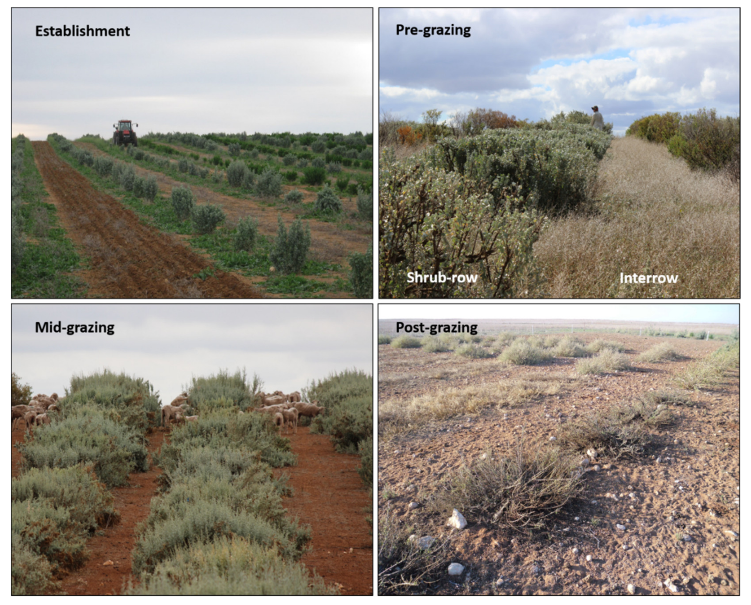
This study was composed of two parts: the development of a module for APSIM to allow dynamic sheep grazing of plantations of saltbush with an interrow, and by way of demonstration of the versatility of application, an investigation of a range of options currently available to farmers to manage saltbush plantations for livestock production. Figure 1 shows a managed saltbush plantation typical of the LRZ of southern Australia was investigated.

2.1. Overview

The saltbush model [16] operating within the APSIM model framework v.7.9 [17] was used to generate edible plant biomass in response to daily weather conditions, as well as the growth and edible biomass accumulation of pastures and crops growing in the interrow area. Figure 2 shows the important elements of the study that include the daily simulation of plant growth and defoliation and feed allocation.

In the modelling, shrubs were sequentially defoliated and the interrow biomass removed to simulate daily grazing. To achieve this, the energy requirements of grazing animals were calculated, then based on simulations of shrubs and interrow net growth and biomass accumulation, the metabolizable energy (ME) available from the different sources were calculated, and then the selection of this ME was apportioned according to the grazing/browse behaviour of a flock of sheep. The analysis used a generic grazing animal, in this case a non-lactating sheep of 50 kg in size (a dry sheep equivalent, DSE) with a daily energy requirement of 8.5 MJ/DSE/day. The daily amount of forage removed was calculated according to aspects of livestock energy demand and intake of the animals [18], feed availability, assumptions regarding diet selection and predicted feed intake. Where deficits of ME occurred, these were filled with supplementary feeding. Details of the modelling and assumptions in the analysis are outlined below.

2.2. Simulating Grazing of Saltbush Systems with Interrow Plants

The saltbush model employed two distinct zones: the saltbush zone, coinciding with the shrub-row where the saltbush is planted, and the interrow zone, coinciding with the area between the shrub-rows. Saltbush roots had restricted access to the neighbouring interrow. For a more detailed explanation see [16]. To represent grazing in APSIM, defoliation of shrubs or interrow plants was simulated using computer programming scripting language C#, called Manager2. The proportion of saltbush selected by the sheep each day was determined according to the digestibility (organic matter digestibility, OMD) of the edible saltbush and interrow plants. The basis for selection came from field studies in Western Australia [19,20] where it was discovered that the proportion of saltbush edible biomass that was consumed (more correctly termed removed) was predicted by the digestibility of the interrow (Figure 3). Small changes, such as a 5% decline in OMD of the interrow meant an 8% increase in the amount of saltbush removed. The range of the data for Figure 3 were only within the range of 45 to 67.5% OMD of edible interrow.

In cases where the OMD of the interrow was outside of the range shown in Figure 3, saltbush DM removal was set at 54% of the diet if the OMD of the interrow was below 45%, and 12% of the diet if the OMD of the interrow was above 68%. These experimental data highlight how sheep included a proportion of saltbush (average of 13%) in their diets even when highly digestible feed (i.e., a high OMD) was available in the interrow. Under the hypothesis that intake behaviour remained constant, these data were used, to calculate a saltbush intake parameter (as % of DM intake) that was determined by the digestibility of the interrow (or supplementary feed). Once the intake requirements of all animals were calculated, the rates for all animals in a paddock were summed and then allocated between the available feed components in the paddock (i.e., shrub, interrow and supplement). Dry matter digestibility (DMD) of the interrow plants was provided by APSIM on a daily basis and then converted to ME as shown in Equation (1) [18]:

ME (MJ/kg) = (0.172 × DMD%) − 1.707

(1)

In comparison, the APSIM saltbush model is rudimentary and does not calculate the digestibility of the available plant material. Therefore, the estimation of ME for shrubs involved a user-provided value for OMD which was then converted to ME using Equation (2) [18]:

ME (MJ/kg) = 0.169 × OMD − 1.986

(2)

Based on Figure 3, the OMD of the saltbush shrub was fixed a 50% as there was little variation about for all the year. Metabolism crate feeding studies across a range of saltbush species confirmed this figure [21]. A minimum of 50 g shrub leaf biomass was set as the residual and assumed unavailable for grazing. In cases where there was insufficient availability of interrow or shrub to satisfy the animals’ daily energy requirements, supplementary feed of a fixed ME (8.5 MJ/kg DM) was fed in the paddock daily (this was comparable to the commonly used supplementary feeds such as hay). During periods when there was little or no available interrow and supplementary feeding was required, saltbush continued to make up a proportion of the daily diet based on the nominal digestibility of the interrow. In this way using a dynamic calculation of quality of the interrow, daily grazing was represented. However, several other assumptions were necessary:

• Daily intake of saltbush was additional to interrow and selected as Figure 3;
• Animals consumed feed according to daily energy maintenance requirements;
• Potential animal intake was determined by daily animal energy requirements related to the live bodyweight of the animal [22];
• The sheep were accustomed and willing to graze the saltbush [23].

Thereby, using the APSIM models for growth of pastures and crops, the changes of OMD of the interrow were simulated, which in turn defined the amount of saltbush removed by the grazing animals. An important part of the simulation was that the ME of the plant material changes as it transitions through the different plant stages. Additionally, it was assumed that the ground water tables, were sufficiently deep that they did not influence soil hydrology nor plant growth which is supported by [24]. Although saltbush plantations have sometimes been targeted at the rehabilitation of saline soils or those with a high water-tables [25,26,27], this is not always the case and for initial simplicity in the current study, soils were assumed to be non-saline and therefore plant productivity was not limited by osmotic soil effects.

2.3. Systems Scenarios

The modelling-functionality was used to investigate different scenarios of forage systems based on saltbush and different interrow plants. In many cases these scenarios were based on farming systems already in practice [12,13,23]. A system was simulated where the period of grazing was 90 days–starting on 1 February until 30 April–which is common farmer practice in the LRZ. The simulated area was 1 hectare with a shrub density of 769 shrubs/ha (3.0 m between individual plants, and 4.3 m between the shrub-rows). The perennial saltbush was planted as seedlings once at the start of the simulation.

To represent the return of nutrients in excreta, nitrogen (N) was added each day as urea at 25 g N/DSE/day. The initial values for available soil N each were set to 7.4 mg nitrate/kg and 10 mg ammonium/kg within the top 1.0 m soil. To ensure any effect of changes in soil N and organic matter did not confound the comparisons between systems, at the conclusion of the grazing period (i.e., 1 May), a range of model parameters were reset. These included soil N, surface soil OM, edible shrub and interrow biomass, with soil moisture reset to the lower limit (or permanent wilting point).

Simulations were conducted using climate data from 1997 to May 2020. The first 3 years of simulation results were excluded to ensure that the shrubs were mature. For all the systems, the stocking rate was 25 DSE/ha-which is a typical stocking rate when intensively grazing a forage shrub stand.

2.4. Assessing Forage Shrub Systems with Interrow

2.4.1. Locations—Climate and Soils

As the LRZ covers a wide range of regions, simulations were conducted for different climates and soil types to illustrate the versatility of the modelling-functionality. The model was run across three locations in Australia (see Figure S1 in Supplementary Materials): Waitchie #77049 (35.37° S, 143.10° E; average annual rainfall for 2000–2020: 306 mm and decile 2 rainfall or rainfall in the lowest 20% of the simulation period: 195 mm) and Waikerie (34.29° S, 140.03° E; 257 and 143 mm, respectively) in South Australia, and in Western Australia at Kellerberrin #10073 (31.62° S, 117.72° E; 307 and 207 mm, respectively. For each location, daily historical climate data (rainfall, solar radiation, pan evaporation, maximum and minimum temperatures) were extracted from the SILO patched point dataset [28]; http://www.bom.gov.au/silo/ accessed on 22 February 2020). All locations were in the 250–500 mm rainfall, mixed farming zone of Australia and are indicative of the areas where saltbush is grown in managed plantations. According to the classification system used by [29], the zone is mostly a cold semi-arid climate with smaller areas with Mediterranean hot summer climate. Cold semi-arid climates typically have warm to hot dry summers, though their summers are typically not quite as hot as those of hot semi-arid climates. Unlike hot semi-arid climates, areas with cold semi-arid climates tend to have cold winters. However, the climate in this region has changed in recent decades becoming drier and with a shift in the seasonality of rainfall. Therefore, this current analysis focussed on the climate from 2000 onward. Figure 4 indicates how the climate data, averaged for the 20-year period 2000–2019 were similar in terms of seasonal rainfall but that at Kellerberrin, with its Mediterranean climate, had a relatively higher proportion of winter rainfall compared to the other locations.

Details of the soil properties used in the simulations were taken from the APSoil database [30] and are shown in

Table A2. Soil physical and chemical properties used in the simulations (PAWC is for the depth exploited by roots). Bo, OC and pH were used to estimate the rooting depth. PAWC: Plant available water content; BD: bulk density (g/cm³), DUL is drained upper limit (volumetric %); LL is lower limit (volumetric %); EC is electric conductivity (1:5 saturated paste; dS/m); pH (1:5 water); Bo is Boron (mg/kg) OC is organic carbon (%).

Description	PAWC	Root Depth	Test	Depth (mm)
(APSoil #)	(mm/m)	(cm)		10	20	40	60	80	110	140
Waikerie	54	80	BD	1.53	1.68	1.64	1.59	1.66	1.65	1.61
(No. 360)			DUL	0.08	0.07	0.09	0.10	0.17	0.21	0.19
			LL	0.02	0.03	0.04	0.05	0.07	0.14	0.14
			EC	0.1	0.1	0.1	0.2	0.4	0.4	0.4
			pH	7.2	8.5	8.3	8.4	8.6	8.6	8.6
			Bo	2	1.9	2.5	3.7	6.8	17	17
			OC	0.61	0.34	0.23	0.11	0.04	0.03	0.03
Waitchie	119	100	BD	1.25		1.25		1.31	1.31	1.31
(No 718)			DUL	0.33		0.3		0.31	0.37	0.37
			LL	0.12		0.12		0.12	0.12	0.12
			EC	0.1		0.1		0.2	0.3	1.3
			pH	8.4		8.7		8.7	9	8.3
			Bo	1.2		1.1		1.5	3.2	7.1
			OC	0.77		0.62		0.38	0.19	0.12
Kellerberrin	92	110	BD	1.7	1.6	1.6	1.5	1.5	1.4	1.4
(No 406)			DUL	0.14	0.14	0.16	0.20	0.21	0.21	0.21
			LL	0.07	0.07	0.07	0.12	0.12	0.12	0.12
			EC	−	−	−	−	−	−	−
			pH	6.1	5.8	6.5	7.2	7.8	8.3	8.4
			Bo	−	−	−	−	−	−	−
			OC	0.57	0.3	0.2	0.14	0.12	0.1	0.1

in Appendix B. Plantations on non-saline land with sandy soils are common in the LRZ of southern Australia [24] and so similar systems were replicated. The growth of crops and pastures are often constrained by a combination of chemical and physical impediments to root development, low inherent fertility and low water holding capacity. The maximum rooting depth of shrubs, irrespective of location, was set to 1.5 m following the data of [16].

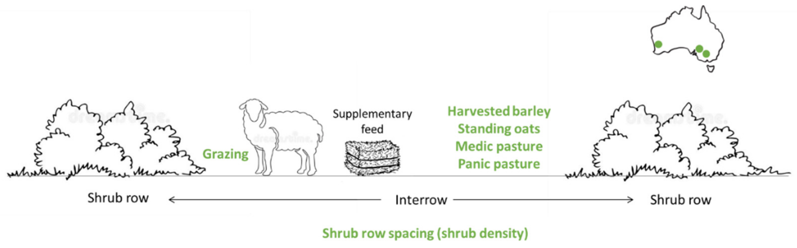
2.4.2. Plant Species in the Interrow

Different interrow pastures and crops shown in

Table 1. Details of the APSIM 7.9 pasture and crop options simulated in interrow. Lifecycle is A—annual; P—perennial.

Plant Name	Lifecycle	APSIM Model	Cultivar
Barrel Medic (Medicago truncatula)	A	AusFarm	Paraggio
Panic (Megathyrsus maximus) 1	P	AusFarm	Gatton
Oats (Avena sativa)	A	Crop	Wintaroo
Barley (Hordeum vulgare)	A	Crop	Hindmarsh

¹ unreleased parameter set from [31].

were simulated. These included an annual medic and a perennial species, temperate and tropical pasture and annual crop species. Barrel medic (Medicago truncatula) is the most common self-regenerating annual pasture legume in the LRZ, whereas panic grass (Megathyrsus maximus) is a relatively newer tropical perennial species with limited areas sown in comparison. Simulations of pastures were conducted using the AusFarm pasture models in APSIM. These were run as established pastures-meaning that the sward was mature from the start of the simulation and therefore it was not necessary to sow the pasture. Simulations of crops were conducted using the APSIM crop models and unreleased parameter set from [31]. Oats (Avena sativa) and barley (Hordeum vulgare) crops were sown between the 7 May and 7 July when at least 20 mm of rain fell over a 5-day period to produce a population of 150 plants/m² in rows 30 cm apart. At sowing, 30 kg of N fertiliser as urea was applied. The simulations assumed that no species other than those shown were present at any time.

All plants were grazed, but oats were grazed as a standing crop (i.e., grain in the head was removed rather than mechanically harvested), whereas the barley was harvested when ripe and therefore only stubble, otherwise called crop residue was available for grazing. For initially simplicity, it was assumed that only the crop leaf and grain material was available for consumption by the livestock. Additionally, in the case of barley, 2% of the crop grain yield was assumed to be spilt during harvest and was thereby also available for consumption. The digestibility of all plant material was defined as shown in

Table A1. Dry matter digestibility (DMD, %) of different interrow pasture species and different plant parts. Note the oats grain was 65% digestible (or 9.5 MJ/kg).

	Green		Dry		Litter/Dead
	Leaf	Stem	Leaf	Stem	Leaf	Stem
Medic	75	65	50	40	40
Panic	65	55	50	40	40
Winter Weed	70	60	40	30	30
Oats	-	-	40	25	40	25
Barley	-	-	40	25	40	25

in Appendix A. From field observations, the edible saltbush material was assumed to be all leaf material and 5% of stem material, i.e., the young and palatable, stem material.

Shrub-Row Spacing

The effects of the different interrow species with varying shrub densities were compared. The different shrub-row densities were achieved by varying the width of the interrow area; thereby reducing the number of shrubs per hectare with larger distances for the interrow. The distance between the shrub-rows was modified to produce either 1000 shrubs/ha (3.0 m between shrub rows), 769 shrubs/ha (4.5 m), 500 shrubs/ha (8 m) or 250 shrubs/ha (18 m). A simulation was also conducted without any shrubs.

2.4.3. Timing of Grazing

Different regimes for the timing of grazing over a period of 90 days were simulated. These regimes were implemented for the pastures (i.e., medic, panic grass) growing in the interrow only and not for the crops (i.e., barley, oats). The same plantation configuration was used as detailed in Section 2.1: a shrub density of 769 shrubs/ha (3.0 m between individual plants, and 4.3 m between the shrub-rows).

A so called ‘common’ grazing time was started on 1 February which is commonly when farm feed-gaps are at their most severe and grazing of shrubs commonly begins on many farms. The other grazing systems were termed based on their starting date: 1 January—‘summer’ and 1 April—‘autumn’. In all three cases, this was same system (i.e., same grazing period, same shrub density, same starting date of 1 February) as described above with either medic (winter active) or panic (summer active) interrow to provide contrast.

A ‘dual’ grazing system was simulated with two grazing periods. There was a full 90-day grazing (starting at 1 September or 1 February) or two 45-day periods (starting at 1 September and 1 February). The other variation was where sheep started grazing 1 February but were removed if there was no shrub or interrow biomass remaining. All of these above variations in the ways and timing of shrub-plantations with an interrow are grazed are important as these are examples of actual systems occurring in the low rainfall zone [12,13].

2.5. Data Analysis

As the value from saltbush plantings to the farming systems are highly dependent on seasonal conditions, both the average biomass production, supplementary feed requirements etc, and indicators of variability of the same are presented. As the value of saltbush plantation is arguably greatest during low rainfall periods when there is little available forage on other parts of the farm, the data for those periods were analysed apart from the longer-term averages. Thus, low rainfall or dry periods were denied as the model output during the lowest 20% of simulation years in the 12-month period prior to the commencement of grazing.

Many famers use the saltbush plantations to maintain livestock until more nutritious annual pastures become available on the rest of the farm as rains in late autumn bring conditions favourable for plant growth. If other forage options are not available, then livestock need to be fed with supplemental feeding to maintain bodyweight. Therefore, supplementary feed requirements are also reported for comparison between the different systems simulated.

3. Results

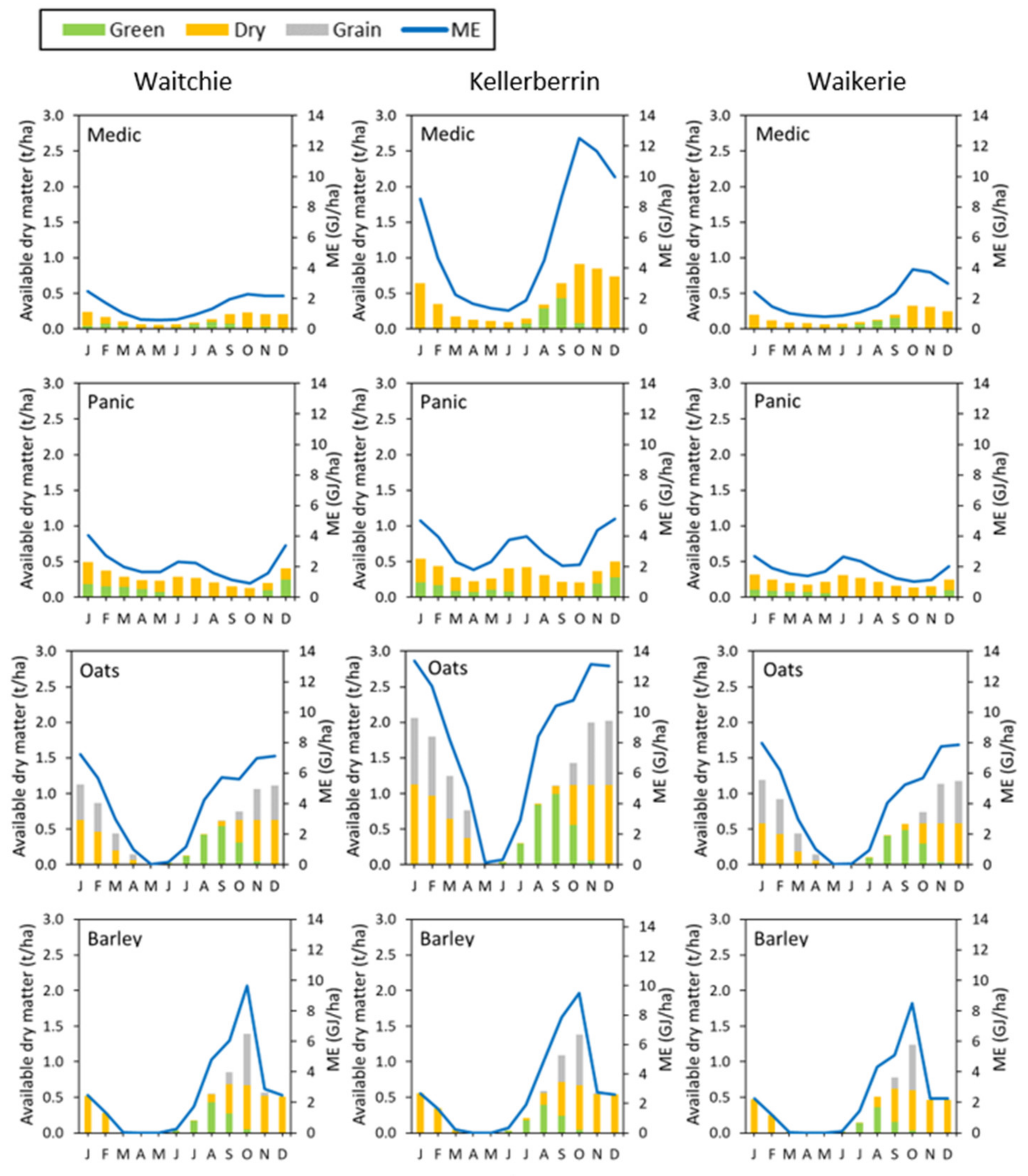
3.1. System Simulation Demonstration

As a demonstration of the capability of the modelling functionality, examples of the simulated daily dynamics of available shrub and interrow with daily consumption, over a range of years at Waitchie are shown in Figure 5.

At Waitchie, the period covered the twelve-month period leading up to the start of February in which years 2017 and 2018 were in the top 20% of simulation years, and years 2016, 2019 and 2020 were in the lower 20% of simulation years.

Figure 6 shows the simulation results of the 90-day grazing periods at Waitchie, for a subset of the 20-year dataset. It indicates the variability of the farming systems between years and the versatility of the modelling in simulating these integrated systems. The low rainfall years (lowest 20% of years) are recognizable as they require supplementary feeding even in cases where the interrow consisted of unharvested crops. Additionally, the years with high rainfall and resultant high biomass production were evident as they required comparatively less supplementary feed. (The corresponding results for Figure 5 and Figure 6 are shown in the Supplementary Materials for Figures S2 and S4 for Kellerberrin as well as Figures S3 and S5 and Waikerie).

Saltbush dry matter was more reliably available for consumption than medic-based interrow during the February to May period. There was several years where low rainfall resulted in an absence of interrow pasture (medic) availability during the grazing period. Figure 4 shows how the interrow medic pasture was removed early in the grazing period leading to a reliance on supplementary feed to maintain bodyweight for the remainder of the period. On average, saltbush comprised 30% of the dry matter removed over the grazing periods, but years such as 2003 and 2007 show that saltbush availability was also prone to be inadequate in some years, leading to almost total dependence on supplementary feed by the end of the grazing period.

3.2. Designing Farming Systems Based on Forage Shrubs

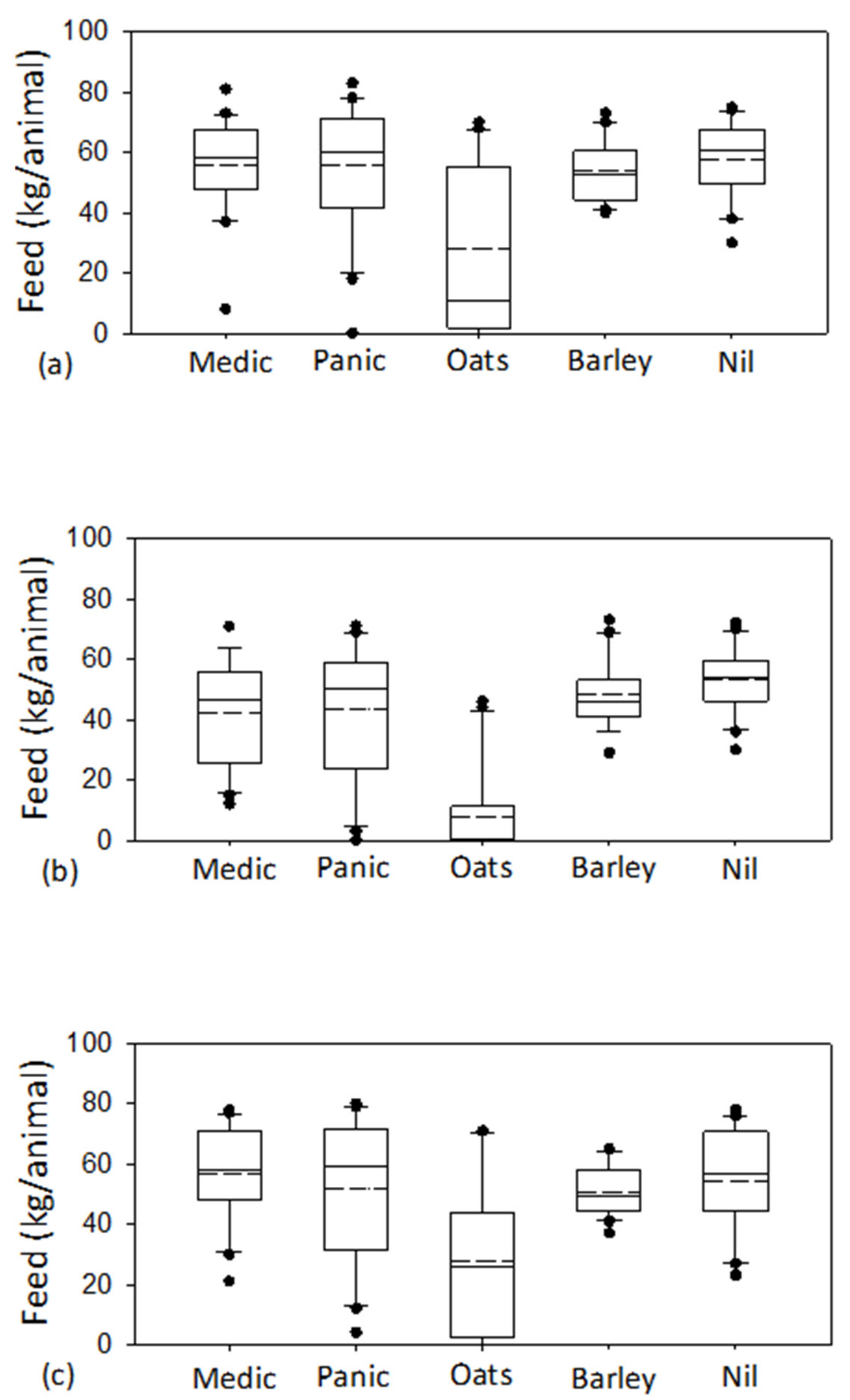
3.2.1. Different Interrow Plant Options

There were obvious differences in the annual growth cycles of the pastures and crops over the period of an average year between locations. Not only in terms of the growth of biomass, but also the amount of dead, dry or green dry matter differed between systems with different interrow species and between locations (Figure 7).

Overall, there was similar growth of interrow species at Waikerie and Waitchie, however the growth was distinctly different at Kellerberrin. Given the widespread use of the shrub systems for summer feed, the availability of dry matter, or more importantly ME in January/February is a logical basis for comparison between systems with different species, location and years. This did not translate into the same magnitudes of available ME as panic is of lower digestibility. The difference between average years and low rainfall years was more notable for medic however, reflecting the temperature growth cycle and shallower rooting compared to panic. At that time for medic, the average ME density of the available dry matter was higher at Kellerberrin (9.3 MJ/kg DM) than at Waikerie (7.3 MJ/kg DM) and Waitchie (7.2 MJ/kg DM) even though the plant material was dead.

Although barley had a large amount of digestible dry matter throughout the year, once harvested the feed available for livestock was similar to panic in terms of dry matter and with similar or lower ME. Overall, the predicted unharvested oats was greatest, dry matter and of higher quality even during dry periods.

Table 2. Feed on offer (GJ ME/ha) on 1 February (day 31) available of shrub and different interrow species after lowest 20% rainfall year at Waitchie (2006, 2015, 2018, 2002), Waikerie (2006, 2015, 2018, 2002) and Kellerberrin 2000, 2001, 2002, 2010).

	Medic		Panic		Oats		Barley
	Shrub	Interrow	Shrub	Interrow	Shrub	Interrow	Shrub	Interrow
Waitchie	6.1	2.0	5.5	1.2	5.0	7.2	5.3	3.7
Waikerie	5.8	5.5	5.5	4.2	4.7	9.0	6.1	3.5
Kellerberrin	5.8	5.5	5.5	2.9	6.0	10.6	5.5	2.1

shows the feed on offer at the start of the grazing period for the different locations and interrow species. As the stocking rate was fixed across all systems and locations the amount of residual dry matter at the end of the 90-day grazing period differed.

Unexpectedly, during these low rainfall periods the ME calculated by panic interrow was less than for medic and roughly similar to harvested barley. In comparison, systems with unharvested oats in the interrow was more than double that of barley.

Overall, across all locations and systems, the interrow was more variable overall with a CV of 36% in dry years whilst the interrow is 64%.

Supplementary Feed Requirements

Figure 8 shows the effects of different plant species growing in the interrow area on the annual supplementary feed requirements.

Oats was the most successful interrow option in terms of reducing the requirement for supplementary feed. The reliance on supplementary feeding varied greatly between locations due to the amount and seasonal patterns of rainfall. For example, at Kellerberrin and Waitchie the different shrub and interrow had very different biomass production, not only due to differences in rainfall amounts but largely due to the seasonality of rainfall and temperature regimes. The site in Western Australia at Kellerberrin, had the least seasonal variability in dry matter production from the shrub/interrow system. This resulted in a narrow range in variability in supplementary feeding.

The standing oat crops had long term average grain yields (grain was grazed in the ear rather than harvested) ranging from 1.4 t/interrow ha at Kellerberrin, down to 0.9 t/interrow ha at Waikerie and Waitchie. This additional 0.5 t DM/interrow ha at Kellerberrin provided a significant amount of the feed requirements especially where supplementary feed was often required in small amounts. The harvested barley crop system had a similar mean supplementary feed requirement to the system based on a panic interrow. Additionally, at most locations the systems with a medic interrow had a higher feed requirement compared to systems with panic.

In the very dry years (i.e., low 20% of rainfall years in the simulation period) there was little difference between the pasture species although systems with a panic interrow did require slightly less supplementary feed during these periods. As per other times, an oat crop was the interrow that required the least supplementation.

For the Waitchie example shown, at the start of the grazing period the availability of interrow was significantly more variable (long term coefficient of variation, CV, of 1.28) than the shrub leaf biomass (CV of 0.50). Including both shrub and interrow medic meant a long-term CV of 0.50 for the reliance of on supplementary feed.

Of the scenarios investigated: shrub plantations with an interrow of standing oats required least supplementation (21 kg/sheep on average across all locations), compared with those with panic grass (50 kg) which were highly variable between years (coefficient of variation of 44%), whereas those with barley crop stubbles were the least variable (CV 20%).

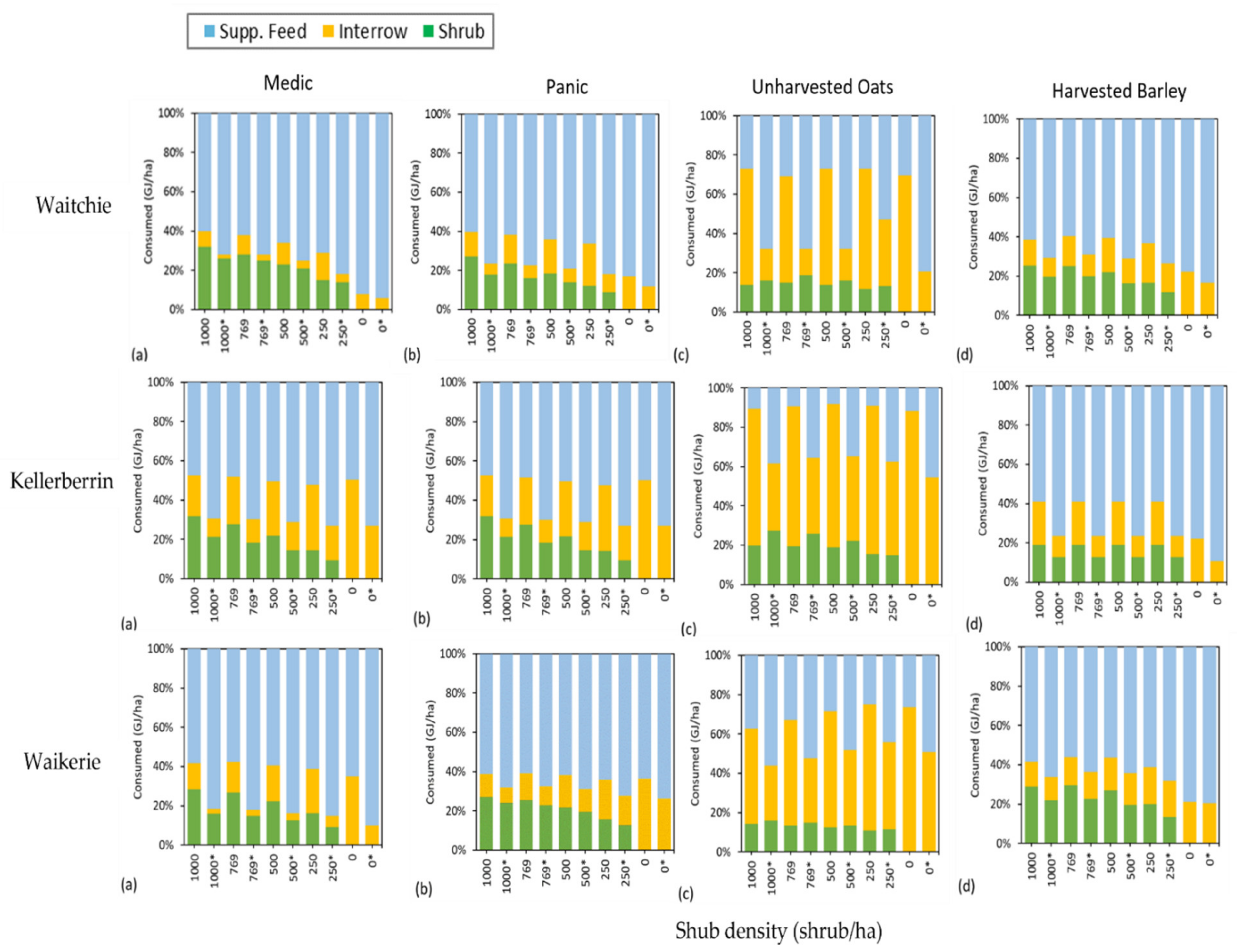
3.2.2. Varying Plantation Shrub Density

There were several ways in which the diet composition (i.e., proportion of shrub, interrow, supplementary feed) was influenced by variations in the density of shrubs and the diet therefore also varied with location (i.e., soil type, climate), shrub density and rainfall years as shown in Figure 9. Having greater amount of interrow pasture reduced the average supplementary feed requirement, however the reliability across years decreased.

For medics, across all locations there was a reduction in the proportion of shrub removed relative to increasing shrub density. The effect was greatest at Waitchie both in average and in low rainfall years which are indicated by an asterisk in Figure 9. However, these relative differences due to density and climate were greater in at other locations. At Kellerberrin, the differences due to shrub density in the proportional composition of the diet were negligible, even in low rainfall years. In average rainfall years at Waitchie and Waikerie, more than half of the diet during the 90-day grazing period came from supplementary sources. In low rainfall years, having medic in the interrow effectively did not reduce the supplementary feed requirement.

Panic pastures followed the same responses as medic pastures to increasing shrub density and rainfall years. The effect of shrub density on the proportion of supplementary feed removed was negligible in average rainfall years relative to shrub density, but with an increase in the proportional consumption of panic pastures resulting in a decline in shrub consumption. This was consistent between the systems with pasture interrow.

For systems with standing oat crops, the proportional differences in the diets between average and low rainfall years was less than the pasture systems. The proportion of shrubs in the diet increased in low rainfall years, when the availability of the crop was less. For systems with harvested barley crops in the interrow, the supplementary feeding requirements in average years was greater than in systems with oats at Waitchie, but in dry years similar. At Kellerberrin however, in dry years the supplementary requirement was more than two thirds of the diet. At Waitchie and Waikerie, in general proportionally more shrubs were removed in systems with interrow of barley compared to standing oats.

3.2.3. Different Grazing Regimes

Focussing on Waitchie, the effects of different starting times for the 90-day grazing period were compared in the systems with perennial summer growing grass (panic) and annual winter growing grass (medic).

Table 3. Feed removed from different sources (i.e., shrubs, pasture or supplementary feed) for a panic and medic pasture over 90-day periods starting in low rainfall years (lowest 20% of simulation period) at the three study locations. Dual shows the total amount for the full grazing period. Dual ^a sheep are removed if there was no shrub or interrow biomass remaining in the October grazing period; Dual ^b sheep are retained for the full period on both occasions.

		Common	Summer	Autumn	Dual a	Dual b
	Units	(1 February)	(1 January)	(1 April)	(1 October/1 April)
Waitchie				Panic
Shrub removed	GJ/ha	4.6	3.3	2.5	1.4	2.7
Pasture removed	GJ/ha	4.7	2.5	2.5	3.3	1.7
Supplementary feed	kg/sheep	46	63	67	6	21
		Medic
Shrub removed	GJ/ha	4.6	5.0	4.4	2.7	2.1
Pasture removed	GJ/ha	0.0	0.0	0.0	0.7	1.6
Supplementary feed	kg/sheep	68	66	70	23	29
Kellerberrin				Panic
Shrub removed	GJ/ha	5.1	3.6	2.9	1.8	2.6
Pasture removed	GJ/ha	3.8	1.8	3.6	2.7	0.2
Supplementary feed	kg/sheep	48	65	60	3.0	28
		Medic
Shrub removed	GJ/ha	4.4	3.6	2.9	1.4	3.2
Pasture removed	GJ/ha	1.8	1.8	3.7	2.7	0.3
Supplementary feed	kg/sheep	61	64	59	15	26
Waikerie				Panic
Shrub removed	GJ/ha	5.1	4.8	2.3	4.0	1.1
Pasture removed	GJ/ha	3.8	4.5	5.4	0.0	0.0
Supplementary feed	kg/sheep	48	47	54	21	0.0
Kellerberrin				Panic
Shrub removed	GJ/ha	5.1	4.8	2.6	3.0	3.2
Pasture removed	GJ/ha	3.8	4.6	4.5	0.0	0.0
Supplementary feed	kg/sheep	48	46	56	0.0	2.4

shows how the differences in the active growth periods of the different species (shown in Figure 7) affected the supplementary feed requirements. (The reader should note that the amount of supplementary feed is given on a weight basis (i.e., kg) as that is most meaningful to farmers, however this could also have easily been conveyed on a ME basis and is easily converted as the density was 8.5 MJ/kg DM as outlined above).

For single duration period grazing, the results show that grazing forage shrub systems in summer–early autumn (January–March) was likely to be most valuable as they required the least supplementary feed. However, the requirements for supplementary feed were not measurably different between the two different pasture species for grazing starting in January. For the common grazing in February, systems with a medic interrow required 50% more feed and in the dual grazing system where sheep are removed if there was no shrub or interrow biomass remaining in the October grazing period, was the lowest overall at 6 kg per sheep or almost 4 times that of systems with panic interrow.

Apart from the late autumn grazing period (beginning 1 April) which required the highest amounts of supplementary feed at 70 kg/sheep due to the low interrow forage availability (shown in Figure 7) during this time for the medic interrow, however there was effectively little difference between grazing regimes. The 4 kg difference between the low in summer and high in autumn is unlikely to be significant in the long term.

4. Discussion

Although this study focussed on three locations in the low rainfall zone of Australia as an illustrative example of the capability of the modelling functionality, the methodology is transferrable to other areas of the world where managed forage shrub plantations with an interrow are used such as semi-arid and arid regions of Asia, Africa and the Americas. There are many similarities with regard to the use of forage shrubs, climate and soils between all these areas [5,14]. The current study was based on saltbush but can be expanded to include other Atriplex spp. or forage shrubs such as legume tagasaste (Chamaecytisus proliferus) as APSIM models are developed. It is likely that with hotter, drier and more variable conditions under a changing future climate, that the viability and sustainability of many farms in the low rainfall zones will be tested further, and therefore it is important to have a systems perspective to compare the value of alternative farming systems.

4.1. Interrow Plant Options

The livestock production potential of saltbush plantations can be undervalued by only assessing the productivity of the saltbush shrubs alone. Much of the overall plant productivity can come from the interrow area and it has been shown that even small changes in diet digestibility of the order of 1% can result in live weight changes in livestock [32]. Yet, despite the recognised importance of the interrow in forage shrub systems, no previous study has investigated a range of potential interrow species, shrub plantings or different grazing times to compare productive combinations in terms of total complementary feed value for livestock at different grazing times over a wide range of season types.

An unstated objective of the systems design was to highlight the potential of different systems with the least residual saltbush and/or interrow, and the most cost-effective systems, in terms of input costs. The modelling analysis showed that the choice of interrow species and the density of shrubs are important considerations to reduce the need for costly supplementary feeding. Grazing sown crops was the best option for the interrow with the least requirement for supplementary feed in summer-autumn. However, this does not consider costs of sowing, fertilising, spraying and harvesting which when taken into consideration against pasture options, may make it less attractive. The design process therefore is aided using such a flexible framework that can direct attention towards farming systems for more focussed investigations. For example, this modelling was based on existing, mature pastures and in reality, tropical grasses can be very difficult to establish in low rainfall locations [33] that might change the feasibility of the potential farming system.

Differences in shrub density, together with physical differences due to the variations in the proportional areas occupied by shrubs and interrow created different grazing systems. The systems with relatively more saltbush had a greater reliance on supplementary feed over the long term, but the seasonal variation in supplementary feed required was less as shrub density increased owing to the stable production of edible shrub biomass between years. The study also illustrated that the inclusion of saltbush in the diet during autumn might reduce the need for supplementary feed but does not completely obviate it. From a biological perspective as the salt content of saltbush (up to 25% DM) provides a consumption constraint to sheep and cattle and they need a non-saline dietary component [5,19]. Supplementary feeding was still necessary to ensure that the daily energy requirements are met in cases when there was insufficient available interrow for grazing. These results illustrate a production dilemma: the better (i.e., more digestible) the interrow, the less the shrubs are removed which typically resulted in more residual shrub dry matter (i.e., remaining at the end of the grazing period). This unutilised resource feed resource could be viewed as wasted. Alternatively, any green leaves that are on the shrubs are using soil moisture and this assists with management of dryland salinity in discharge areas. In cases where there was little accompanying interrow there was a greater need for supplementation. Reducing the availability of supplementation rather than ad libitum, might encourage greater consumption of the saltbush. However, this means more intensive management. The overall message is that the objective should be to synchronise as closely as possible the termination of available feed of both the shrubs and the interrow without the use of costly supplementation. This can be achieved through the selection of species and even cultivars with different nutritional profiles and through management (i.e., fertilization). A lower quality of the interrow would make the animals more inclined to graze the saltbush. This understanding was clear from the scenario modelling but had been less obvious beforehand.

4.2. Decision Support for Farming Systems Design

The current study has shown that the modelling functionality in APSIM is able to accommodate many of the commonly utilised interventions that would be helpful in systems design. Whilst the intention was never to do a sensitivity analysis, the results discussed above will vary with the decisions to reset the systems (i.e., in terms of soil water, biomass, soil carbon, soil nitrogen, etc.), stocking rate decisions, animal type and shrub type. However, the modelling would be suited to this analysis where necessary. In systems where the building up of saltbush forage over a number of seasons to create reserves (a “drought insurance” for livestock) was necessary–the use of the reset would be unsuitable. Our conclusions from the utilisation of the modelling-functionality concur with the conclusions of [34] whom, modelling silvopastoral systems, considered the higher level objective of their modelling system was to help make consistent choices and compare different systems and management regimes, rather than to produce very accurate predictive values of sward or tree production. Therefore, the modelling functionality presented, is better employed as decision support for farming systems design, as opposed to a model to reproduce the specific responses of actual systems, for example, under experimentation. In this sense, this modelling capability is an important tool for testing ideas and scenarios. This is particularly valuable, as the design, implementation and analysis of integrated forage systems, such as those based on saltbush, are expensive and difficult to carry out in practice and require long time frames, and potentially can have differing outcomes depending on the types of rainfall years during the experimental period.

Addressing a holistic system that deals with interactions between different forage plants, animals and management practices over multiple years is a valuable aspect of the system. Due to the variability of the climate zones in which the forage shrub plantations are utilized, long time frames are required to assess the overall suitability of different farming systems as forage systems respond differently in different rainfall years. Considering the high variability of rainfall between years for the sites in this study (e.g., Waitchie coefficient of variation of annual rainfall is 41%), addressing the responses of the systems in different rainfall years is important when designing forage systems. These scenario analyses could be part of a of larger and more comprehensive, full farming systems analysis however, that incorporates economics and different soil types such [35].

Beyond soft-testing of the model outcomes, it is arguably impossible to validate the modelling, as such datasets do not exist. Additionally, other site characteristics not included in the modelling would also complicate comparisons between simulated and experimental data. For example, [19] found over the course of one year that the daily growth rate of saltbush in terms of edible dry matter, ranged from 0.6–5.6 g dry matter/day/shrub. These daily growth rates were less than those in the simulations of growth. However, in the case of [19] the experimental site was described as a highly salt-affected soil above extremely saline groundwater which was likely to have significantly restricted potential growth. Deliberately, the effects of soil salinity and elevated water tables were not included in the current modelling. Additionally, the choice to reset the system annually was suitable for the current study which explored the productive potential of various scenarios as they related to different climate years. However, in reality the effect of end-on-end simulations on forage available, soil water, soil carbon and N pools over multi-year runs is important. Therefore, meaningful comparisons across studies are difficult as the effects of soil type, extent of soil fertility limitation, and rainfall as well as climate patterns on shrub growth can be considerable. Nevertheless, the study found potentially edible saltbush dry matter, on offer in summer-autumn, was often less than 1 t dry matter/ha which agreed with data from a survey of farms in the low rainfall regions of South Australia [24] and measured at Pithara, Western Australia [36].

4.3. Modelling Integrated Forage Systems

Although a few conceptually similar biophysical models for integrated grazing systems such as silvopastoral systems exist [34,37,38,39,40], none have attempted to use models to explore a livestock focus on forage shrub systems. This study has demonstrated that this new model-functionality for the APSIM framework can be valuable for the analysis of forage systems where saltbush and/or other woody perennials are important. However, we are fully cognisant that adequately representing animal grazing behaviour is fraught as it is influenced by many biophysical and behavioural factors, as many other factors, influence intake and selection [41]. In many cases the systems researchers above have also been challenged in a similar way to the current study: that pre-existing and individually validated components (viz. the saltbush and dynamic grazing) are brought together in a larger model that then requires proper evaluation. Whilst this is the case for many systems models, there are no available datasets of daily grazing behaviour, daily changes in plant growth and digestibility, together with defoliation and animal weight changes, to test this model and therefore the predictive ability beyond sensibility of the outputs and dynamics remains unresolved. This lack of rigorous validation is a clear weakness of this study and remains difficult to resolve as research on grazing systems in the drylands continues to be poorly researched, poorly funded and difficult to conduct. Nevertheless, the modelling approach could be used to address systems where preferential grazing of multiple feed sources occurs or other polyculture systems such as agroforestry.

With the accumulation of further experimental information a more comprehensive sensitivity analysis would be possible. This is necessary to challenge some of the assumptions in the current model about for example the relationships between grazing behaviour and digestibility, interactions between plants growing in the different zones, animal production responses to the different feeds, growth patterns of the plants under different edaphic conditions and many more. Nevertheless, this is a poorly funded area of research and therefore the accumulation of such information is slow and piecemeal. Therefore, the modelling is best used to understand potential system behaviour and changes, however a sensitivity analysis could and should be the subject of a future study.

Animal intake is a function of biomass availability and a function of factors such as physical and chemical characteristics of the feed that include fibre breakdown rate and/or salt [42]. The modelling framework was not comprehensive in terms of animal production and future versions could incorporate growing animals (with dynamic weight and energy requirements) or forages with variable salt content. One reason that the effect of salt was not included in the analysis was that we focussed on factors that farmers can modify through management. The relationship in Figure 3 needs to be tested and redefined for a range of shrub types that vary in terms of digestibility and salt content to increase the functionality even further. Despite these potential limitations, the outputs from the model can be used to inform graziers to plan grazing systems in response to seasonal variation in production by different feed sources or can be used by scientists to form hypotheses which can be tested in field experiments.

5. Conclusions

In the harsh, low rainfall zones of the world, managed plantations of forage shrubs are a way to sustain livestock through periods of feed gaps. However, in the variable climate of the LRZ, defining diverse, resilient and productive forage systems to sustain the livestock over the long term, continues to be challenging. Managing a shrub system for livestock can be complex and requires information on the digestibility of the shrubs and interrow plants. The new functionality modelling framework developed in this study can be used to efficiently and comprehensively explore various options to help reduce supplementary feeding and optimise the livestock production, as well as potentially be applied to other integrated forage and agroforestry systems. The inclusion of saltbush increased the overall livestock production potential of the pasture area and reduced the interannual variability in feed supply, compared to only having a pasture species or grazed annual crop species. The study indicates the importance of interrow grazing in shrub systems but also suggests that in shrub-interrow systems, there will still be a requirement for supplementary feeding when grazed over longer summer-autumn periods. The amount of feeding depends on location, rainfall year, species and configuration of the plantation. Most importantly, this study advances our understanding of how to functionally reproduce the behaviour of integrated systems.

References

1. Moore, A.D.; Bell, L.W.; Revell, D.K. Feed gaps in mixed-farming systems: Insights from the Grain & Graze program. Anim. Prod. Sci. 2009, 49, 736–748. [Google Scholar]
2. Le Houerou, H.N. Utilization of fodder trees and shrubs in the arid and semiarid zones of West Asia and North Africa. Arid Soil Res. Rehabil. 2000, 14, 101–135. [Google Scholar] [CrossRef]
3. Nefzaoui, A. The integration of fodder shrubs and cactus in the feeding of small ruminants in the arid zones of north Africa. In Livestock Feed Resources within Integrated Farming Systems; FAO: Rome, Italy, 1996; pp. 467–483. [Google Scholar]
4. El Shaer, H.M. Adaptation to climate change in desertified lands of the marginal regions in Egypt through sustainable crop and livestock diversification systems. Sci. Cold Arid Reg. 2015, 7, 16–22. [Google Scholar]
5. Ben Salem, H.; Norman, H.C.; Nefzaoui, A.; Mayberry, D.E.; Pearce, K.L.; Revell, D.K. Potential use of oldman saltbush (Atriplex nummularia Lindl.) in sheep and goat feeding. Small Rumin. Res. 2010, 91, 13–28. [Google Scholar] [CrossRef]
6. Abu-Zanat, M.W.; Ruyle, G.B.; Abdel-Hamid, N.F. Increasing range production from fodder shrubs in low rainfall areas. J. Arid Environ. 2004, 59, 205–216. [Google Scholar] [CrossRef]
7. Monjardino, M.; Revell, D.; Pannell, D.J. The potential contribution of forage shrubs to economic returns and environmental management in Australian dryland agricultural systems. Agric. Syst. 2010, 103, 187–197. [Google Scholar] [CrossRef]
8. Thomas, D.T.; White, C.L.; Hardy, J.; Collins, J.P.; Ryder, A.; Norman, H.C. An on-farm evaluation of the capability of saline land for livestock production in southern Australia. Anim. Prod. Sci. 2009, 49, 79–83. [Google Scholar] [CrossRef]
9. Mirza, S.N. Fodder Shrubs and Trees in Pakistan; International Center for Agricultural Research in the Dry Areas (ICARDA): Aleppo, Syria, 2000; pp. 153–177. [Google Scholar]
10. Zucca, C.; Pulido-Fernandez, M.; Fava, F.; Dessena, L.; Mulas, M. Effects of restoration actions on soil and landscape functions: Atriplex nummularia L. plantations in Ouled Dlim (Central Morocco). Soil Tillage Res. 2013, 133, 101–110. [Google Scholar] [CrossRef]
11. Papanastasis, V.P.; Yiakoulaki, M.D.; Decandia, M.; Dini-Papanastasi, O. Integrating woody species into livestock feeding in the Mediterranean areas of Europe. Anim. Feed Sci. Technol. 2008, 140, 1–17. [Google Scholar] [CrossRef]
12. Mallee Sustainable Farming. Saltbush in the farming system. The farmer’s perspective. In Case Studies of Four Farmers Who Are Successfully Using Saltbush on Their Farms; Mallee Sustainable Farming: Mildura, VIC, Australia, 2014; p. 8. [Google Scholar]
13. Rural Solutions. Strategic Practical Options for Intergrating Cropping and Livestock Systems: A Case by Case Study of 20 Successful Mixed Farming Enterprises in the South Australian Mallee; Primary Industries and Resources of South Australia: Murray Bridge, Australia, 2009. [Google Scholar]
14. Abu-Zanat, M.M.W.; Titi, H.H.; Akash, M.W.; Al-Antary, T.M. Effect of planting forage shrubs and barley on attributes of natural vegetation in arid lands. Fresenius Environ. Bull. 2020, 29, 4777–4788. [Google Scholar]
15. Gintzburger, G.; Bounejmate, M.; Nefzaoui, A. Fodder shrub development in arid and semi-arid zones. In Proceedings of the Workshop on Native and Exotic Fodder Shrubs in Arid and Semi-Arid Zones, Hammamet, Tunisia, 27 October–2 November 1996; p. 299. [Google Scholar]
16. Descheemaeker, K.; Smith, A.P.; Robertson, M.J.; Whitbread, A.M.; Huth, N.I.; Davoren, W.; Emms, J.; Llewellyn, R. Simulation of water-limited growth of the forage shrub saltbush (Atriplex nummularia Lindl.) in a low-rainfall environment of southern Australia. Crop Pasture Sci. 2014, 65, 1068. [Google Scholar] [CrossRef]
17. Holzworth, D.P.; Huth, N.I.; deVoil, P.G.; Zurcher, E.J.; Herrmann, N.I.; McLean, G.; Chenu, K.; van Oosterom, E.J.; Snow, V.; Murphy, C.; et al. APSIM-Evolution towards a new generation of agricultural systems simulation. Environ. Model. Softw. 2014, 62, 327–350. [Google Scholar] [CrossRef]
18. Standing Committee on Agriculture. Feeding Standards for Australian Livestock: Ruminants; CSIRO Australia: East Melbourne, Australia, 1990; p. 256. [Google Scholar]
19. Norman, H.C.; Wilmot, M.G.; Thomas, D.T.; Barrett-Lennard, E.G.; Masters, D.G. Sheep production, plant growth and nutritive value of a saltbush-based pasture system subject to rotational grazing or set stocking. Small Rumin. Res. 2010, 91, 103–109. [Google Scholar] [CrossRef]
20. Fancote, C.R.; Norman, H.C.; Williams, I.H.; Masters, D.G. Cattle performed as well as sheep when grazing a river saltbush (Atriplex amnicola)-based pasture. Anim. Prod. Sci. 2009, 49, 998–1006. [Google Scholar] [CrossRef]
21. Norman, H.C.; Revell, D.K.; Mayberry, D.E.; Rintoul, A.J.; Wilmot, M.G.; Masters, D.G. Comparison of in vivo organic matter digestion of native Australian shrubs by sheep to in vitro and in sacco predictions. Small Rumin. Res. 2010, 91, 69–80. [Google Scholar] [CrossRef]
22. Freer, M.; Moore, A.D.; Donnelly, J.R. GRAZPLAN: Decision support systems for Australian grazing enterprises--II. The animal biology model for feed intake, production and reproduction and the GrazFeed DSS. Agric. Syst. 1997, 54, 77–126. [Google Scholar] [CrossRef]
23. Future Farm Industries. Perennial Forage Shrubs Providing Profitable and Sustainable Grazing. In Key Practical Findings from the Enrich Project; Future Farm Industries CRC: Crawley, Australia, 2014; p. 45. [Google Scholar]
24. Llewellyn, R.; Whitbread, A.; Lawes, R.; Raisbeck-Brown, N.; Hill, P. Fork in the road: Forage shrub plantings by crop-livestock farmers in a low rainfall region of southern Australia. In Proceedings of the Australian Agronomy Conference, Lincoln, New Zealand, 15–18 November 2010; p. 3. [Google Scholar]
25. Norman, H.C.; Masters, D.; Silberstein, R.; Byrne, F. Achieving profitable and environmentally beneficial grazing systems for saline land in Australia. Options Mediterraneennes. Ser. A Semin. Mediterr. 2008, 79, 85–88. [Google Scholar]
26. Barson, M.M.; Abraham, B.; Malcolm, C.V. Improving the productivity of saline discharge areas: An assessment of the potential use of saltbush in the Murray-Darling Basin. Aust. J. Exp. Agric. 1994, 34, 1143–1154. [Google Scholar] [CrossRef]
27. Masters, D.G.; Norman, H.C.; Barrett-Lennard, E.G. Agricultural systems for saline soil: The potential role of livestock. Asian-Australas. J. Anim. Sci. 2005, 18, 296–300. [Google Scholar] [CrossRef]
28. Jeffrey, S.J.; Carter, J.O.; Moodie, K.B.; Beswick, A.R. Using spatial interpolation to construct a comprehensive archive of Australian climate data. Environ. Model. Softw. 2001, 16, 309–330. [Google Scholar] [CrossRef]
29. Peel, M.C.; Finlayson, B.L.; McMahon, T.A. Updated world map of the Koppen-Geiger climate classification. Hydrol. Earth Syst. Sci. 2007, 11, 1633–1644. [Google Scholar] [CrossRef]
30. Dalgliesh, N.P.; Foale, M.A. Soil Matters—Monitoring Soil Water and Nitrogen in Dryland Farming; Agricultural Production Systems Research Unit: Toowoomba, Australia, 1998. [Google Scholar]
31. Descheemaeker, K.; Llewellyn, R.; Moore, A.; Whitbread, A. Summer-growing perennial grasses are a potential new feed source in the low rainfall environment of southern Australia. Crop Pasture Sci. 2014, 65, 1033–1043. [Google Scholar] [CrossRef]
32. Cochrane, M.J.; Radcliffe, J.C. Effect of long-term hay storage on dry-matter, digestible dry-matter and crude protein. J. Aust. Inst. Agric. Sci. 1977, 43, 151–153. [Google Scholar]
33. Smith, A.P.; Llewellyn, R.S. Defining sowing windows for tropical grasses in the low rainfall zone. In Proceedings of the 17th Australian Agronomy Conference, Building Productive, Diverse and Sustainable Landscapes, Hobart, Australia, 20–24 September 2015; p. 4. [Google Scholar]
34. Balandier, P.; Bergez, J.-E.; Etienne, M. Use of the management-oriented silvopastoral model ALWAYS: Calibration and evaluation. Agrofor. Syst. 2003, 57, 159–171. [Google Scholar] [CrossRef]
35. Finlayson, J.D.; Lawes, R.A.; Metcalf, T.; Robertson, M.J.; Ferris, D.; Ewing, M.A. A bio-economic evaluation of the profitability of adopting subtropical grasses and pasture-cropping on crop-livestock farms. Agric. Syst. 2012, 106, 102–112. [Google Scholar] [CrossRef]
36. Morcombe, P.; Young, G.; Boase, K. Grazing a saltbush Atriplex maireana stand by Merino wethers to fill the autumn feed-gap experienced in the Western Australian wheat belt. Aust. J. Exp. Agric. 1996, 36, 641–647. [Google Scholar] [CrossRef]
37. Bergez, J.E.; Etienne, M.; Balandier, P. ALWAYS: A plot-based silvopastoral system model. Ecol. Model. 1999, 115, 1–17. [Google Scholar] [CrossRef]
38. Gillet, F.; Besson, O.; Gobat, J.M. PATUMOD: A compartment model of vegetation dynamics in wooded pastures. Ecol. Model. 2002, 147, 267–290. [Google Scholar] [CrossRef]
39. Gillet, F. Modelling vegetation dynamics in heterogeneous pasture-woodland landscapes. Ecol. Model. 2008, 217, 1–18. [Google Scholar] [CrossRef]
40. Zhai, T.; Mohtar, R.H.; Gillespie, A.R.; von Kiparski, G.R.; Johnson, K.D.; Neary, M. Modeling forage growth in a Midwest USA silvopastoral system. Agrofor. Syst. 2006, 67, 243–257. [Google Scholar] [CrossRef]
41. Wallis, R.H.; Thomas, D.T.; Speijers, E.J.; Vercoe, P.E.; Revell, D.K. Short periods of prior exposure can increase the intake by sheep of a woody forage shrub, Rhagodia preissii. Small Rumin. Res. 2014, 121, 280–288. [Google Scholar] [CrossRef]
42. Arnold, G.W.; Dudzinski, M.L. Studies on diet of grazing animal. 3. Effect of pasture species and pasture structure on herbage intake of sheep. Aust. J. Agric. Res. 1967, 18, 657–666. [Google Scholar] [CrossRef]
Figure 1. A forage shrub system typical of the arid lands, whereby shrubs are established as seedlings in rows and an interrow of plants is maintained.
Agronomy 12 02348 g001
Figure 2. Conceptual overview of the study. Sheep graze the shrub, interrow and supplementary feed (i.e., hay) based on metabolizable energy requirements. Scenarios of different systems (indicated in green) were investigated that included different locations, grazing regimes, shrub density (determined by different interrow width) and interrow plants.
Agronomy 12 02348 g002
Figure 3. (Left) Saltbush removed as proportion of total diet (DM basis) based on organic matter digestibility (OMD) of the understorey/interrow, (right) OMD of the edible saltbush (solid triangle, segmented line) remains relatively constant throughout the year compared to the interrow (open square, solid line) reproduced from [19].
Agronomy 12 02348 g003
Figure 4. (left) Average seasonal rainfall for 2000–2020 (dark columns) and average rainfall of the lowest 20% of simulation years (open columns) and (right) average daily maximum (top of column) and minimum temperature (bottom of column) for (a) Waitchie, (b) Kellerberrin, and (c) Waikerie.
Agronomy 12 02348 g004
Figure 5. Daily change in dry matter (kg/ha) available to animals in the shrub-row (solid line and during the grazing period green shading) and interrow (segmented line and during the grazing period yellow shading) based on APSIM saltbush grazing model with short-term grazing at Waitchie for (a) medic, (b) panic, (c) unharvested oats, and (d) harvested barley. The blue columns indicate supplementary feed. The yellow shading of the segmented line indicates periods when grazing occurred. All plants were reset to a common threshold at the end of the grazing period.
Agronomy 12 02348 g005
Figure 6. The proportional daily amount of saltbush shrub (green columns), interrow (yellow columns) and supplementary feed (blue columns) in the total diet for (a) medic pasture, (b) panic pasture, (c) unharvested oats, and (d) harvested barley for Waitchie with a defined 90-day grazing period February 1 to May 1 each year. Note: These are stacked column graphs with each day of the year shown to indicate the different feed sources during the grazing period and between years. The blank area indicates the 275-day period when there was no grazing.
Agronomy 12 02348 g006
Figure 7. Long term average, monthly (January to December) standing green (green bar) and senesced (yellow bar) biomass, and available metabolizable energy (line) of the animal-available dry matter for annual legume (medic), perennial Panic grass, crop (standing, unharvested oats and harvested barley) at Waitchie (first column), Kellerberrin (middle columns) and Waikerie (last columns) with 769 shrubs/ha. Grey bars indicate the harvested barley grain. Note the data are for non-defoliated interrow and have been reset annually to a common residual dry matter at the start of May.
Agronomy 12 02348 g007
Figure 8. Long-term annual supplementary feed requirements at (a) Waitchie, (b) Kellerberrin and (c) Waikerie. Boxes indicate the 25 and 75th percentiles, whiskers (error bars) indicate the 90th and 10th percentiles, line within the box the median, segmented line the mean. Nil indicates system with no interrow plants, only shrubs.
Agronomy 12 02348 g008
Figure 9. Average annual, proportional diet composition based on total energy (GJ/ha) for shrub (green columns), interrow (yellow columns) and supplementary feed (blue columns), for different shrub densities (shrubs/hectare) indicated on the x-axis at the three study sites (Waitchie, Kellerberrin, Waikerie) based on shrub systems with an interrow of (a) medic, (b) panic, (c) unharvested oats and (d) harvested barley. Columns with asterisk (*) indicate the average of the years during low rainfall-lowest 20% of the simulation period.
Agronomy 12 02348 g009