Climate-Based Modeling and Prediction of Rice Gall Midge Populations Using Count Time Series and Machine Learning Approaches

Abstract

The Asian rice gall midge (Orseolia oryzae (Wood-Mason)) is a major insect pest in rice cultivation. Therefore, development of a reliable system for the timely prediction of this insect would be a valuable tool in pest management. In this study, occurring between the period from 2013–2018: (i) gall midge populations were recorded using a light trap with an incandescent bulb, and (ii) climatological parameters (air temperature, air relative humidity, rainfall and insulations) were measured at four intensive rice cropping agroecosystems that are endemic for gall midge incidence in India. In addition, weekly cumulative trapped gall midge populations and weekly averages of climatological data were subjected to count time series (Integer-valued Generalized Autoregressive Conditional Heteroscedastic—INGARCH) and machine learning (Artificial Neural Network—ANN, and Support Vector Regression—SVR) models. The empirical results revealed that the ANN with exogenous variable (ANNX) model outperformed INGRACH with exogenous variable (INGRCHX) and SVR with exogenous variable (SVRX) models in the prediction of gall midge populations in both training and testing data sets. Moreover, the Diebold–Mariano (DM) test confirmed the significant superiority of the ANNX model over INGARCHX and SVRX models in modeling and predicting rice gall midge populations. Utilizing the presented efficient early warning system based on a robust statistical model to predict the build-up of gall midge population could greatly contribute to the design and implementation of both proactive and more sustainable site-specific pest management strategies to avoid significant rice yield losses.

1. Introduction

Rice is the staple food crop for more than half of the world’s population. The Asian gall midge, Orseolia oryzae (Wood-Mason) (Cecidomyiidae: Diptera) (Figure 1a), is one of the most common difficult-to-control rice pests in South and Southeast Asia [1,2,3]. In India, it is the third most important rice pest after the stem borer and the plant hoppers [2], affecting 30–70% of the total rice area [4]. It is most prevalent in the states of Andhra Pradesh, Telangana, Tamil Nadu, Kerala, Goa, Karnataka, Maharashtra, Madhya Pradesh, Bihar, Odisha, Assam, Manipur, and in certain niches of West Bengal, and Uttar Pradesh of India [5,6,7,8]. The gall midge completes its life cycle in 19–23 days at 22 to 28 °C and about 85% humidity. In April and May, pre-monsoon rains in India amplify insect activity in rice stubble, self-sown rice, and other hosts. The late planted rice varieties receive extensive damage. Insect activity peaks between the last week of August and the first week of October. Graminaceous weeds (Leersia hexandra and Echinochloa crus-galli) and wild rice varieties (Oryza nivara, O. barthii, and O. rufipogon) serve as alternate hosts [6]. Younglings feed on the shoot meristem during the tillering stage of crops, resulting in the formation of a tubular structure called ‘silver shoots’ (Figure 1b). The affected tillers fail to bear panicles. Yield losses caused by the gall midge are highly variable depending on the severity of attack; however, in extreme cases, complete yield loss of crop is possible. In Southern India alone, yield loss due to gall midge was estimated to be about 0.8% of total yield or approximately US$ 80.00 million [2]. Besides the inherent biotic potential of insects, to a large extent, abiotic factors determine the abundance of insect pests in a crop ecosystem. Therefore, an efficient early warning system based on a robust statistical model to predict gall midge population buildup is of great importance in designing and implementing a proactive and more sustainable site-specific pest control and management strategy.

Count time series modeling is a popular statistical approach in which integer autocorrelated discrete count observations are considered as inputs, and the observations are assumed to be derived from Poisson and negative Binomial distributions. Crop pest modeling is one of the major areas of count time series modeling wherein daily or weekly counts of insects (pests), which are autocorrelated in nature, are considered. Though count time series models and machine learning techniques are applied in different areas, application of these techniques is novel for the modeling and forecasting of gall midge populations. Some of the count time series models were applied: in stock exchange data [9,10], monthly claims count of workers in the heavy manufacturing industry data [11], monthly strike count time series [12], Campylobacterosis infections count time series [13,14], prediction of number of dengue incidents in Jakarta [15], and network traffic count time series [16]. Ref. [17] reviewed regression- and machine learning-based crop pest prediction methods. Refs. [18,19] developed hybrid time series and machine learning models for crop yield predictions.

The machine learning models were employed in the prediction of various agricultural fields: prediction of oil seed production [20], banana yield prediction [21], rice yield prediction [22,23], prediction of rice pests [24], prediction of early blight severity in tomato crop [25], and prediction of sugarcane borer disease [26].

Predicting rice gall midge populations based on climatological parameters greatly aids the take up of preventive crop protection measures. However, past works on forecasting insect pest populations were mostly limited to multiple regression analysis and classical time series models. For count data that follows non-Gaussian distribution; Poission and negative binomial, transformation to normality does not improve the accuracy of the prediction model. Despite the generalized linear model (INGARCH) being better suited for count data, their applications are limited in the field of pest modelling [27,28]. For highly heterogeneous and nonlinear data, prediction models like multiple linear regression and auto regressive integrated moving average models were also reported to be not effective [20,21]. However, machine learning models such as SVR, and ANN could be effective in such conditions as they are assumption-free and data driven.

Modeling and forecasting of insect pest populations is used to provide an aid in decision making and in planning of crop management activities adequately. However, the present work is undertaken to develop a robust statistical model for predicting gall midge populations based on climatological input parameters that are crucial for in life cycles of this rice pest using count time series and machine learning approaches. The models were developed to predict gall midge population to minimize the yield losses. For the first time, we have applied the count time series model, i.e., INGARCH, with weather variables in insect pest modelling area of agriculture, revealing few applications of machine learning models in modeling and forecasting pest populations in general. However, the gall midge prediction is the first attempt in modeling and forecasting using machine learning techniques like ANN and SVR.

The methodological framework begins with basic descriptive statistics, correlation analysis, and stepwise regression analysis to understand the causal relationships between gall midge populations and input variables. Advanced computational methods, such as INGARCH, ANN and SVR with exogenous weather variables, are developed to model and predict gall midge populations in Indian hot spots.

2. Materials and Methods

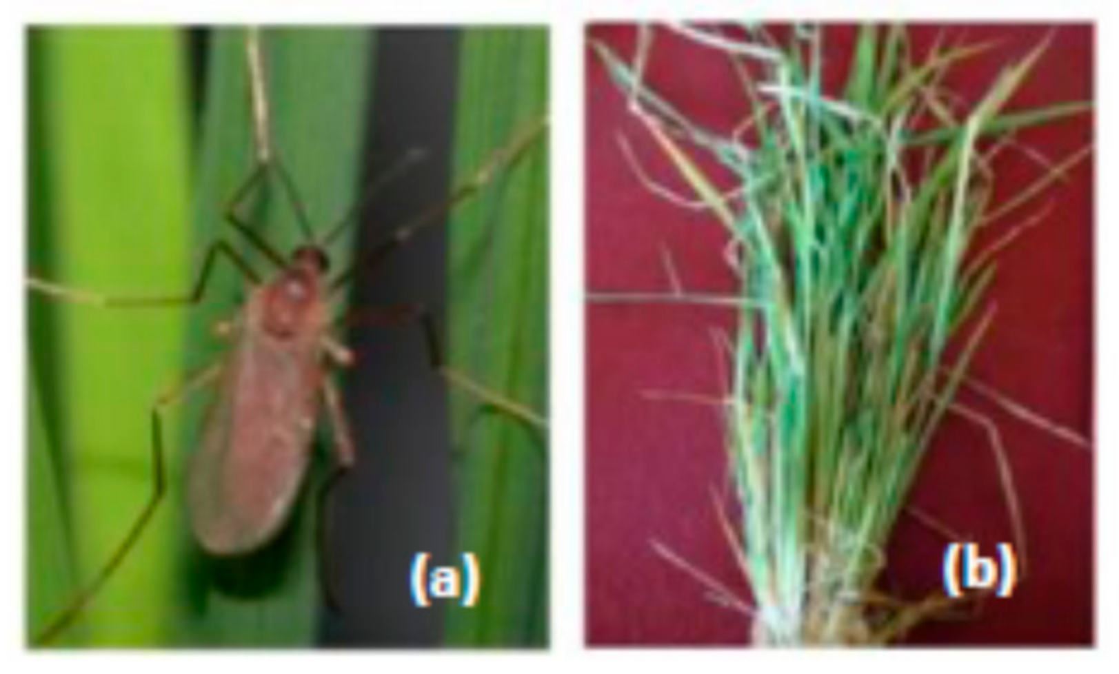
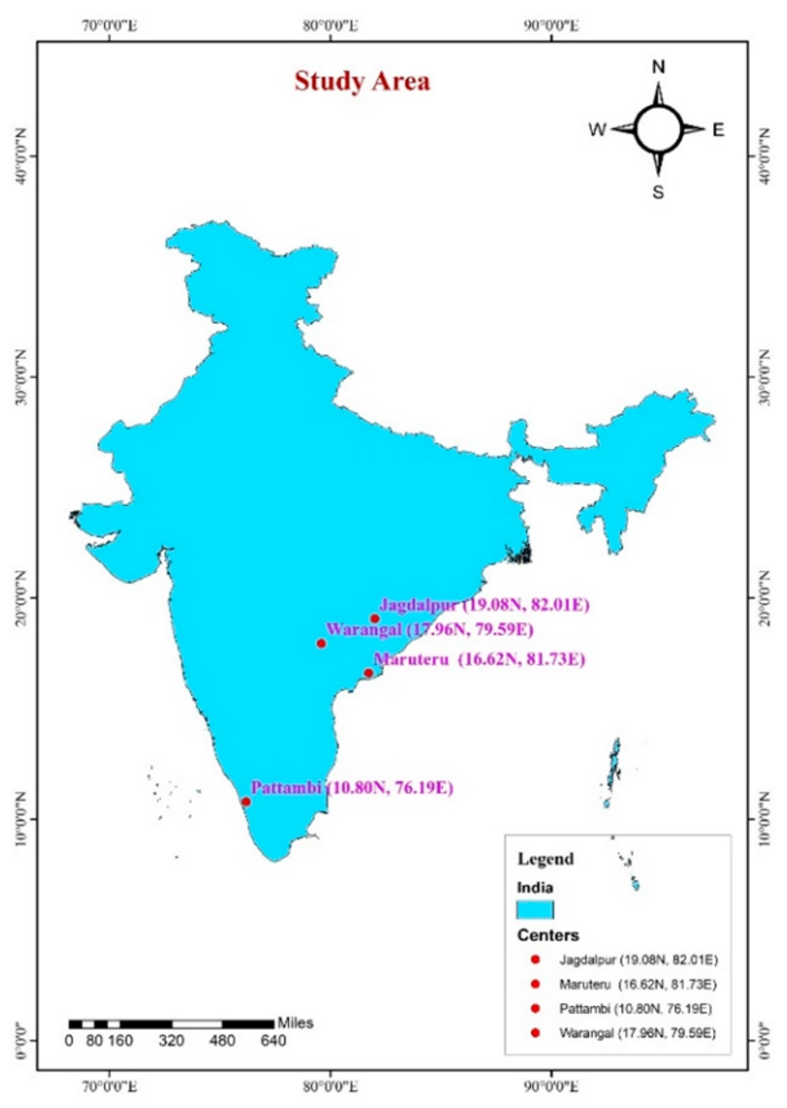
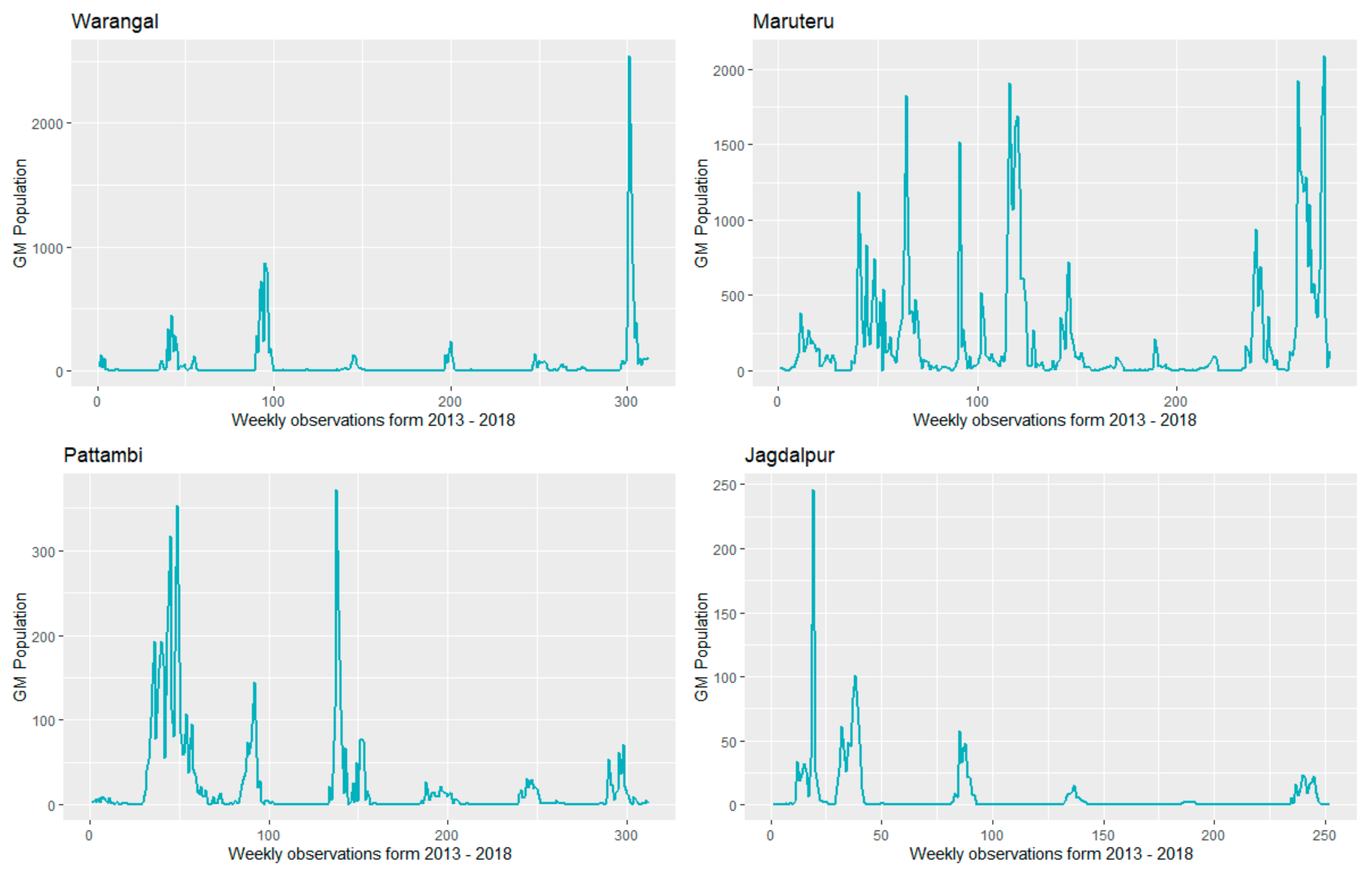
2.1. Data Collection

The Chinsurah type light trap with a 200-watt bulb was used in the study because it is successfully used in monitoring of rice gall midge and other insect pests in rice ecosystems throughout the year [29,30]. The bulb was illuminated daily from 6:00 pm to 6:00 am. In the morning, the collected rice gall midges were brought to the laboratory and the number of individuals caught per day were manually counted, summed and presented as weekly cumulative catches [31]. If the insect catches were too large, the population was divided into different equal subgroups, one subgroup was counted and then multiplied with the remaining number of subgroups. Data were collected at four hot spot locations in India: Warangal, Maruteru, Pattambi and Jagdalpur (Figure 2). Corresponding climatological data on maximum temperature (MAXT), minimum temperature (MINT), total rainfall (RF), morning relative humidity (RHM), evening relative humidity (RHE) and sunshine hours (SSH) were also collected from automatic weather stations at the respective locations. Standard meteorological week (SMW)-wise cumulative catches of gall midge and weekly averages of climatological parameters were considered for this study. Six-week observations were used as testing/validation sets, and remaining observations were used as the training data set.

2.2. Statistical Models

Statistical modeling started with descriptive statistical parameters encompassing mean, standard error (SE), skewness, kurtosis, minimum observation, maximum observation, and coefficient of variations (CV), which are important in depicting the nature of the studied data. Apart from the descriptive statistics, data were depicted graphically with time series plots. Pearson’s product moment correlation analysis was carried out to determine the interrelationship among the variables used in the study. Stepwise, a multiple regression analysis was done to understand the cause-and-effect relationship among the gall midge populations and exogenous weather variables. The regression equation in terms of matrix notation can be expressed as;

$$Y=X\beta +e$$

(1)

where, $Y$ is the variable, $X$ is the vector of exogenous variables, $\beta$ is the regression coefficient vector, and $e$ is the residuals term assumed to be normally distributed with $e~N\left(0,{\sigma }^2\right)$. The time series plots, INGARCH, ANN and SVR models were developed in R software (R Core Team 2018). Correlation analysis and stepwise regression analysis were carried out in SAS 9.3 version [32], available at ICAR-Indian Institute of Rice Research, Hyderabad, India.

2.2.1. Integer-Valued Generalized Autoregressive Conditional Heteroscedastic (INGARCH) Model

The time series following the generalized linear model (GLM) framework was elaborated by [33]. INGARCH models are the class of GLM [34,35], in which the conditional distribution of dependent variable is assumed to follow popular discrete distributions like Poisson, negative binomial, generalized Poisson and double Poisson distributions [10].

Let the count time series be $\left\{Y_t: t\in N\right\}$ and time varying r-dimensional covariate vector say $\left\{X_t: t\in N\right\}$ i.e., $X_t={\left(X_{t,1, }\dots ,X_{t,r, }\right)}^T$. The conditional mean becomes $E\left(Y_{t }\left|F_{t-1}\right.\right)={\lambda }_t$ and F_t is historical data. The generalized model form is expressed as follows:

$$g\left({\lambda }_t\right)={\beta }_0+{{\displaystyle \sum }}_{k=1}^p{\alpha }_k \stackrel{\sim }{g}\left(Y_{t-i_k}\right)+{{\displaystyle \sum }}_{l=1}^q{\beta }_{l}g ({\lambda }_{t-\mathrm{jl}})+{\eta }^T$$

(2)

Case 1: Consider the situation where $g$ and $\tilde{g}$ are equal to identity, i.e., $g\left(x\right)$=, $\tilde{g}\left(x\right)=x$. Further, $Y_t$ follows (Poisson) INGARCH (p, q) model with p > 1 and q ≥ 0 if

(a)

$Y_t$ conditioned on $Y_{t-1}, Y_{t-2}, \dots ,$ is Poisson distributed

(b)

The conditional mean ${\lambda }_t=E\left[\left.Y_t\right|Y_{t-1}, Y_{t-2}, \dots , \right]$ satisfies

$${\lambda }_t={\beta }_0+{{\displaystyle \sum }}_{i=1}^p{\alpha }_i Y_{t-i}+{{\displaystyle \sum }}_{j=1}^q{\beta }_{j }{\lambda }_{t-j} \mathrm{with} {\beta }_0>0 and {\alpha }_1 , \dots , {\alpha }_{p }, \dots , {\beta }_1 , \dots , {\beta }_{q }\ge 0$$

(3)

Assuming further that $Y_t\left|Y_{t-1}\right.$ is Poisson distributed, then we obtain an INGARCH model of order p and q, abbreviated as INGARCH (p, q) model. If q = 0, the model can be referred to as the INAGARCH (p) model. These models are also known as autoregressive conditional Poisson (ACP) models [9].

Case 2: The negative binomial distribution allows for a conditional variance to be larger than the mean ${\lambda }_t$, which is often referred to as over-dispersion (with overdispersion parameter $\varnothing$) [36]. It is assumed that $Y_t\left|F_{t-1}~NegBionom(\right.{\lambda }_t,\varnothing )$. When $\varnothing \to \infty$, the Poisson distribution is a limiting case of the negative binomial distribution by the assumption:

$$\left.Y_t\right|Y_{t-1}, Y_{t-2}, \dots ,~Bin\left(n, \beta +\alpha \frac{Y_{t-1}}{n}\right)$$

(4)

Further details about INGARCH model estimation using conditional likelihood estimation, especially on asymptotic properties, are given by [34] and [37]. The standard INGARCH model allows forecasts to be made based on only past values of the forecast variable. The model assumes that future values of a variable depend on its past values and values of past exogenous variables. The INGARCHX model is an extended version of the INGARCH model [38].

2.2.2. Support Vector Regression (SVR)

The principal idea involved in SVR is to transform the original input space into high dimensional variable space and then build the regression or time series model in a transformed high dimensional feature space [39]. A vector of data set says $Z={\left\{x_{i }{y}_i\right\}}_{i=1}^N$, where $x_i\in R^n$ is the input vector, y_i is the scalar output, and N is the size of data set. The general equation SVR can be written as follows:

$$f\left(x\right)=W^T\varphi \left(x\right)+b$$

(5)

where, W is weight vector, b is bias term, and superscript T denotes the transpose. The coefficients W and b are estimated from data by minimizing the following regularized risk function:

$$R\left(\theta \right)=\frac{1}{2}{\parallel w\parallel }^2+C\left[\frac{1}{N}{{\displaystyle \sum }}_{i=1}^N{L}_{\epsilon }\left(y_i,f\left(x_i\right)\right)\right]$$

(6)

This regularized risk function minimizes both the empirical error and regularized term simultaneously, which helps in avoiding both under and overfitting of the model. In Equation (8), the first term $\frac{1}{2}{\parallel w\parallel }^2$ is called the ‘regularized term’, which measures the flatness of the function. Minimizing $\frac{1}{2}{\parallel w\parallel }^2$ will make a function as flat as possible. The second term $\frac{1}{N}{{\displaystyle \sum }}_{i=1}^N{L}_{\epsilon }\left(y_i,f\left(x_i\right)\right)$ is called the ‘empirical error’, which was estimated by Vapnik ε-insensitive loss function as follows:

$$L_{\epsilon }\left(y_i,f\left(x_i\right)\right)=f\left(x\right)=\left\{\begin{array}{c}\left|y_i,f\left(x_i\right)-\epsilon \right|; \left|y_i-f\left(x_i\right)\right|\ge \epsilon ,\hfill \\ 0 \left|y_i-f\left(x_i\right)\right|<\epsilon , \end{array}\right.$$

(7)

where, y_i is actual value and $f\left(xi\right)$ is an estimate value. The most commonly used kernel function is the radial basis function (RBF) which is given as follows:

$$k(x_i, x_j)=exp\left\{-\gamma \parallel x-x_i\parallel {}^2\right\}$$

(8)

The performance of RBF kernel function requires optimization of two hyper-parameters: regularization parameter C, which balances the complexity and approximation accuracy of the model, and the Kernel bandwidth parameter, which represents the variance of the RBF kernel function, $\gamma$. In SVR and ANN also the exogenous variables are used for both modeling and forecasting purposes as in INGARCHX model. Schematic representation of SVR architecture is given in Figure S1.

2.2.3. Artificial Neural Network (ANN)

ANN is the most widely used machine learning technique in the last several decades. In the area of time series modeling, the ANN is commonly referred to as the autoregressive neural network as it considers time lags as inputs. The time series framework for ANN can be mathematically modeled using a neural network with implicit functional representation of time. The general expression for the final output Y_t of a multi-layer feed forward autoregressive neural network is expressed as follows:

$$Y_t={\alpha }_0+{{\displaystyle \sum }}_{j=1}^q{\alpha }_{j}g\left({\beta }_{0j}+{{\displaystyle \sum }}_{i=1}^p{\beta }_{ij}{Y}_{t-p}\right)+{\epsilon }_t$$

(9)

where, ${\alpha }_j\left(j=0,1,2,\dots ,q\right)$ and ${\beta }_{ij}\left(i=0,1,2,\dots ,p, j=0,1,2,\dots ,q\right)$ are the model parameters, also called as the synopsis weights, p is the number of input nodes, q is the number of hidden nodes, and $g$ is the activation function. Training part in ANN minimizes the error function between actual and predicted values. The error function of autoregressive ANN is expressed as follows:

$$E=\frac{1}{N}{{\displaystyle \sum }}_{t=1}^N{(e_t)}^2=\frac{1}{N}{{\displaystyle \sum }}_{t=1}^N{\left\{X_t-(w_0+({{\displaystyle \sum }}_{J=1}^Q{w}_{J}g\left(w_{oj}+{{\displaystyle \sum }}_{i=1}^P{w}_{ij}{X}_{t-i}))\right)\right\}}^2$$

(10)

where, N is the total number of error terms. The parameters of the neural network $w_{ij}$ are changed by an amount of changes in $\Delta w_{ij}$ as $\Delta w_{ij}=-\eta \frac{\partial E}{\partial w_{ij}}$, where, $\eta$ is the learning rate [20,40]. As in INGARCHX and SVRX models, the exogenous variable will also be used to model the pest count, and hence becomes ANNX model. Graphical representation of ANN architecture is given in Figure S2.

2.3. Comparison Criteria

Mean square error (MSE) and root mean square error (RMSE) were used as comparison criteria for the model performance. The mean square error (MSE) is the average of the sum of squared error values and given as:

$$MSE=\frac{{{\displaystyle \sum }}_{i=1}^N{\left(Y_i-\widehat{Y_i}\right)}^2}{N}$$

(11)

RMSE is also known as standard error of estimate in regression analysis, and is given as:

$$RMSE=\sqrt{\frac{{{\displaystyle \sum }}_{i=1}^N{\left(Y_i-\widehat{Y_i}\right)}^2}{N}}$$

(12)

where, $Y_i$ is the actual value, ${\widehat{Y}}_i$ is the predicted value, and N is the number of observations.

2.4. Diebold–Merino Test

The Diebold–Mariano (DM) test is employed to determine the statistical significance difference among the models used, based on the residuals of the models [41]. Consider the residuals of two models as $r_1$ and $r_2$, and $d_i$ is the absolute difference between residuals; $d_i=\left|r_1\right|-\left|r_2\right|$ and the autocovariance function ${\gamma }_k$ is expressed as:

$${\gamma }_k=\frac{1}{n}{{\displaystyle \sum }}_{i=k+1}^n(d_i-\overline{d})\left(d_{i-k}-\overline{d}\right)$$

(13)

The Diebold–Mariano test statistic is expressed as:

$$DM=\frac{\overline{d}}{\sqrt{\left[{\gamma }_0+2{{\displaystyle \sum }}_{k=1}^{h-1}{\gamma }_k\right]/n}}$$

(14)

where, $h=n^{1/3}+1$. For testing of the hypothesis, the null hypothesis (H₀) and the alternative hypothesis (H₁), $H_0=E\left(d\right)=0$ or the forecast accuracy is similar for two models, and $H_1=E\left(d\right)\ne 0$ or the forecast accuracy is different for two models.

3. Results

The time series plots of weekly (SMW wise) counts of gall midge light trap catches of four study sites during the observed 2013–2018 period were plotted in Figure 3. Year-wise time series plots of gall midge populations at all hot spot locations are depicted in Figures S3–S6. The time series plots show that at all examined locations, the gall midge incidence was higher between the 35th to 45th SMWs, except at the Maruteru centre, where it showed two peaks, between the 10th to 20th SMWs and between the 35th to 45th SMWs.

Summary statistics of the dependent variable gall midge population and exogenous weather variables were calculated and presented in

Table 1. Summary statistics of gall midge light trapped individual collections at study locations.

Location	Statistics	Population	MAXT	MINT	RF	RHM	RHE	SSH
Warangal	Mean	42	32.32	20.05	9.96	86.97	55.93	6.55
	S.E.	7.29	0.27	0.27	1.53	0.18	0.55	0.14
	Skewness	4.8	1.07	−0.34	4.44	−1.94	0.2	−0.76
	Kurtosis	24.68	0.23	−1.06	22.63	10.82	−0.68	−0.18
	Minimum	0	25.71	11.29	0	62.29	33	0.31
	Maximum	875	45.93	31	204.7	93.14	80.14	11.11
	CV (%)	303.53	14.52	23.38	271.23	3.74	17.51	36.73
Maruteru	Mean	215	31.03	24.28	14.27	86.37	73.68	6
	S.E.	23.24	0.15	0.19	1.94	0.21	0.23	0.21
	Skewness	2.7	0.78	−0.35	4.11	−0.46	0	4.07
	Kurtosis	7.4	1	−0.57	22.73	0.21	1.15	32.53
	Minimum	0	24.86	16.17	0	75.43	60.71	0.04
	Maximum	2088	39.71	33.57	284.6	93.71	85.71	34.65
	CV (%)	179.76	7.83	12.74	225.77	4.08	5.2	57.08
Pattambi	Mean	22	32.53	23.17	26.24	88.39	58.82	5.95
	S.E.	2.98	0.15	0.11	3.13	0.36	0.85	0.13
	Skewness	3.9	−0.03	0.75	3.04	−1.23	−0.07	−0.55
	Kurtosis	17.66	−0.46	3.36	10.13	1.58	−0.76	−0.64
	Minimum	0	24.89	18.11	0	58.29	17.43	0.19
	Maximum	372	39.09	32.54	340.5	96.86	94	9.7
	CV (%)	238.91	7.97	8.63	210.76	7.27	25.61	39.18
Jagdalpur	Mean	6	30.56	18.64	13.45	89.51	40.49	5.39
	S.E.	1.3	0.24	0.35	1.96	0.48	1.55	0.16
	Skewness	7.43	0.23	−0.65	3.88	−1.79	−0.01	−0.33
	Kurtosis	75.43	1.42	−0.85	17.01	3.02	−0.98	−1.03
	Minimum	0	17.84	6.57	0	57.57	1.91	0.03
	Maximum	246	41.36	27.8	200.9	97.86	91	9.87
	CV (%)	330.76	12.3	29.83	231.81	8.44	60.8	48.04

MAXT: maximum temperature, MINT: minimum temperature, RF: rainfall RHM: morning relative humidity, RHE: evening relative humidity, SSH: sunshine hours.

. For instance, Asian gall midge populations at Warangal, Maruteru, Pattambi and Jagdalpur were 42, 215, 22 and 6, respectively. The number of population oscillates are in a wide range (0–875), leading to a high percentage of CV and an abnormality of data as skewness and kurtosis are out of normal range. Summary statistics of weather variables presented in Table 1 are self-explanatory, showing that data under consideration were highly heterogeneous in nature.

3.1. Correlation Analysis

Pearson correlation coefficients between gall midge populations and considered climatological variables are depicted in

Table 2. Pearson correlation coefficients between gall midge light trapped individual collections and climatological variables at study locations.

Location		Gall Midge	MAXT	MINT	RF	RHM	RHE
Warangal	MAXT	−0.091 (0.1077)
	MINT	−0.055 (0.3254)	0.59 <0.0001
	RF	−0.053 (0.3483)	−0.18 (0.0013)	0.19 (0.0009)
	RHM	0.151 (0.0072)	−0.16 (0.0054)	0.008 (0.8874)	0.194 (0.0006)
	RHE	0.136 (0.0156)	−0.114 (0.0450)	0.56 (<0.0001)	0.41 (<0.0001)	0.32 (<0.0001)
	SSH	0.126 (0.0256)	0.43 (<0.0001)	0.011 (0.8404)	−0.48 (<0.0001)	−0.18 (0.0011)	−0.39 (<0.0001)
Maruteru	MAXT	0.0234 (0.6977)
	MINT	−0.271 (0.653)	0.685 <0.0001
	RF	−0.0647 (0.283)	−0.041 (0.0497)	0.173 (0.0038)
	RHM	0.092 (0.126)	0.250 (<0.0001)	−0.396 (<0.0001)	0.101 (0.0916)
	RHE	−0.0173 (0.774)	0.316 (<0.0001)	0.169 (0.0046)	0.419 (<0.0001)	0.054 (0.369)
	SSH	0.0404 (0.503)	0.0798 (<0.189)	−0.329 (<0.0001)	−0.276 (<0.0001)	0.0904 (0.1331)	−0.424 (<0.0001)
Pattambi	MAXT	−0.206 (0.0002)
	MINT	0.023 (0.6851)	−0.074 0.192
	RF	−0.0101 (0.8585)	−0.4443 (<0.0001)	0.095 (0.0909)
	RHM	0.126 (0.0255)	−0.521 (<0.0001)	0.211 (0.0002)	0.388 (<0.0001)
	RHE	0.612 (0.2442)	−0.759 (<0.0001)	0.251 (0.0002)	0.526 (<0.0001)	0.732 (<0.0001)
	SSH	0.005 (0.9261)	0.689 (<0.0001)	0.188 (0.0008)	−0.580 (<0.0001)	−0.569 (<0.0001)	−0.809 (<0.0001)
Jagdalpur	MAXT	−0.0664 (0.2934)
	MINT	−0.0064 (0.9195)	0.4088 <0.0001
	RF	−0.0213 (0.7364)	−0.1367 (0.0299)	0.3368 (<0.0001)
	RHM	0.1570 (0.0126)	−0.6879 (<0.0001)	−0.4109 (<0.0001)	0.0996 (0.1148)
	RHE	0.1506 (0.0167)	−0.2337 (0.0002)	0.3658 (<0.0001)	0.4056 (<0.0001)	0.1831 (0.0035)
	SSH	0.1058 (0.0937)	0.2182 (0.0005)	−0.5653 (<0.0001)	−0.3894 (<0.0001)	−0.1245 (0.0482)	−0.4686 (<0.0001)

Values in parentheses represent probability values.

. A low positive significant correlation between gall midge population and RHM, RHE and SSH was observed at Warangal. In Pattambi, gall midge populations also showed a low positive significant correlation with RHM. However, correlation with MAXT was of low negative significance. At Jagdalpur, the gall midge population showed a weak significant correlation with RHM and RHE. Similarly, at Maruteru, the correlation between the trapped gall midge individuals and meteorological parameters was weak. Overall, correlation analysis revealed that gall midge population has association with RHM, RHE, RF and SSH of lower magnitude, ascribable to the heterogeneity or high percentage of CV among gall midge populations.

3.2. Stepwise Regression Analysis

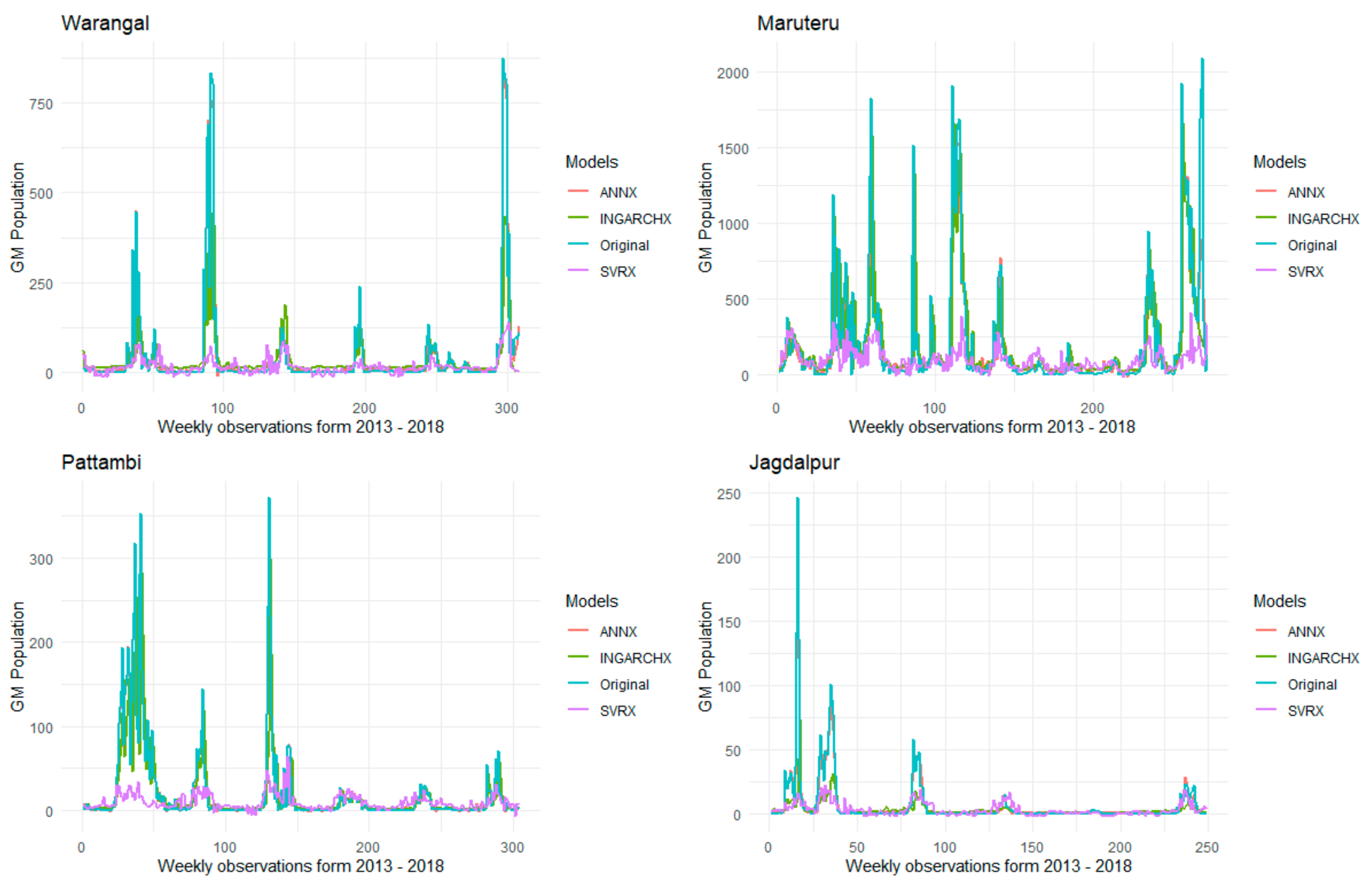
To identify the climatological factors influencing the incidence of gall midge population buildup, a stepwise regression analysis was carried out with the results depicted in

Table 3. Stepwise regression analysis of gall midge light trapped individual collections and climatological variables at study locations.

Centre	Variable	Estimate	S.E.	F Value	Pr > F	R2	Model R2
Warangal	Intercept	−290.71	91.65	10.06	0.0017		0.0854
	MINT	−12.14	3.15	14.88	0.0001	0.0136
	RHE	7.80	1.63	22.84	<0.0001	0.0412
	SSH	22.86	5.49	17.34	<0.0001	0.0854
Maruteru	Intercept	−955.99	745.79	1.64	0.2010		0.092
	RHM	13.79	8.62	2.56	0.0110	0.092
Pattambi	Intercept	−175.75	80.77	4.73	0.0303		0.1010
	MAXT	−8.705	1.723	25.50	<0.0001	0.0427
	RHM	1.534	0.652	5.54	0.0193	0.0844
	RHE	−0.677	0.432	2.46	0.1177	0.0938
	SSH	5.661	2.121	7.12	0.0080	0.1010
Jagdalpur	Intercept	−97.48	25.14	15.04	0.0001		0.1062
	MINT	0.89	0.35	6.57	0.0110	0.0247
	RHM	0.73	0.21	11.73	0.0007	0.0160
	RHE	0.15	0.06	6.51	0.0113	0.0420
	SSH	2.88	0.67	18.27	<0.0001	0.0236

. Some of generated outputs like: (i) MINT, RHE, SSH at Warangal; (ii) RHM at Maruteru; (iii) MAXT, RHM and SSH at Pattambi, and (iv) MINT, RHM, RHE and SSH at Jagdalpur showed significant influence on the gall midge population. Though the listed variables have significant influence on the gall midge populations, the model R² value for the fitted regression in all four of the centers is low, indicating that the model is not a strong fit, for which non-linearity and high heterogeneity in dependent variables may be responsible.

3.3. INGARCHX Model

Prior to subjecting the gall midge individual count time series data into the INGARCH model, the presence of autocorrelation was confirmed by employing the Box-Pierce non-correlation test, and the statistic test revealed a highly significant (p < 0.0001) autocorrelation (

Table 4. Parameter estimation of the INGARCHX model for gall midge populations at study locations.

Centre	Parameters	Estimate	S.E.	Z Value	p	Box-Pierce Non-Correlation Test
						Original	Residuals
Warangal	Intercept	3.63 × 10−5	44.48	8.16 × 10−7	0.9999	${\chi }^2$ = 166.61 p ≤ 0.0001	${\chi }^2$ = 14.24 p = 0.00016
	beta_1	0.46	0.19	2..42	0.0191
	beta_52	0.14	0.12	1.17	0.2604
	MAXT	2.25 × 10−8	0.64	3.52 × 10−8	0.9999
	MINT	7.63 × 10−7	0.78	9.78 × 10−7	0.9999
	RF	6.70 × 10−8	0.08	8.38 × 10−7	0.9999
	RHM	7.90 × 10−8	0.49	1.61 × 10−7	0.9999
	RHE	0.23	0.34	0.6.76	0.5084
	SSH	0.024119	0.87	0.0277	0.9778
	Over dispersion Parameter $\left(\varnothing \right)$	7.32
Maruteru	Intercept	0.0003	412.4300	7.3 × 10−7	0.9999	${\chi }^2$ = 138.96 p ≤ 0.0001	${\chi }^2$= 7.5346 p = 0.00605
	beta_1	0.8519	0.2369	3.600	0.0003
	MAXT	1.48 × 10−5	6.8011	2.2 × 10−6	0.9999
	MINT	2.35 × 10−5	4.7364	5.0 × 10−6	0.9999
	RF	0.2519	0.4708	0.54	0.5926
	RHM	0.1507	2.5737	0.059	0.9533
	RHE	1.19 × 10−9	3.2431	3.7 × 10−10	0.9999
	SSH	2.3553	4.3648	0.54	0.5895
	Over dispersion Parameter $\left(\varnothing \right)$	3.30
Pattambi	Intercept	0.0010	8.1951	0.0001	0.9999	${\chi }^2$ = 190.88 p ≤ 0.0001	${\chi }^2$= 0.109 p = 0.7403
	beta_1	0.7997	0.1950	4.1014	<0.0001
	beta_52	0.0095	0.0159	0.5970	0.5505
	MAXT	2.30 × 10−12	0.2797	8.22 × 10−12	0.999
	MINT	0.0007	0.1898	0.0036	0.9972
	RF	0.0015	0.0075	0.1957	0.8448
	RHM	6.88 × 10−6	0.0581	0.0001	0.9999
	RHE	0.0274	0.0435	0.6325	0.5271
	SSH	3.99 × 10−8	0.2681	1.49 × 10−7	0.999
	Over dispersion Parameter $\left(\varnothing \right)$	2.23
Jagdalpur	Intercept	4.47 × 10−5	3.3598	1.33 × 10−5	0.9999	${\chi }^2$ = 61.29 p ≤ 0.0001	${\chi }^2$ = 6.713 p = 0.0095
	beta_1	0.29454	0.1820	1.62	0.1056
	MAXT	2.34 × 10−12	0.0327	7.16 × 10−11	0.9999
	MINT	0.0032	0.0424	0.0755	0.9404
	RF	0.0178	0.0207	0.86	0.3891
	RHM	4.81 × 10−7	0.0236	2.04 × 10−5	0.9999
	RHE	0.0228	0.0089	2.56	0.0103
	SSH	1.3 × 10−5	0.0870	1.49 × 10−4	0.9999
	Over dispersion Parameter $\left(\varnothing \right)$	5.47

S.E.: standard error, p: probability, ${\chi }^2$: chi square test statistic.

). The INGARCH model with exogenous climatological variables was fitted and the model parameter was found to be significant, but none of the climatological parameters were significant at all hot spot locations. The over-dispersion parameters obtained per location (7.32, 3.30, 2.23 and 5.47) clearly indicated the heterogeneous and over-dispersed nature of the data, following a negative binomial distribution (Table 4). Diagnostic checking of residuals by the Box-Pierce non-correlation test revealed that the residuals were autocorrelated or non-random (p < 0.0001) at all examined locations, except at Pattambi, where the residuals are un-correlated and random in nature (p = 0.7403) (Table 4).

Inability of the INGARCHX model to capture the heterogeneity and complex nature of the data might have led to the non-significant effect of weather variables and significant residuals of the model.

3.4. SVRX Model

The nonlinear SVR model with exogenous variables for the time series of gall midge population count was built with parameter specifications given in

Table 5. Parameter specifications of SVRX and ANNX models for gall midge populations at study locations.

	Warangal	Maruteru	Pattambi	Jagdalpur
SVRX Model
Kernel function	RBF	RBF	RBF	RBF
No. of Support Vectors	139	191	169	107
Cost	1	1	1	1
Gamma	0.16	0.166	0.17	0.170
Epsilon	0.1	0.1	0.1	0.1
Cross validation error	0.024	0.015	0.037	0.033
Box-Pierce non-correlation test for residuals	141.82 (p < 0.001)	123.92 (p < 0.001)	167.16 (p < 0.001)	37.006 (p < 0.001)
ANNX Model
Input lag	4	5	8	3
Dependent/output variable	1	1	1	1
Hidden layer	1	1	1	1
Hidden nodes	6	6	10	10
Exogenous variables	6	6	6	6
Model	10:6S:1L	11:6S:1L	10:10S:1L	9:10S:1L
Total number of parameters	73	79	161	111
Network type	Feed Forward
Activation function I:H	Sigmoidal
Activation function H:O	Identity
Box-Pierce non-correlation test for residuals	0.36 (p = 0.55)	1.003 × 10−6 (p = 0.992)	1.997 (p = 0.157)	1.761 (p = 0.184)

I:H: Input to Hidden layer, H:O: Hidden to Output layer.

. The diagnostic checking of residuals by the Box-Pierce non-correlation test indicated that the residuals are autocorrelated or non-random (p < 0.0001) (Table 5).

3.5. ANNX Model

The ANNX model parameters were given in Table 5 for all the four locations. The gall midge count time series were subjected to the ANN model with 4, 5, 8 and 3 tapped time delays, six exogenous variables, and 6, 6, 10 and 10 optimum nodes for Warangal, Maruteru, Pattambi and Jagdalpur centers, respectively. A sigmoidal activation function in input to hidden layer, and linear identity function in hidden layer to output layer, was used with feed forward network architecture. The total number of parameters or synaptic weights obtained was 73, 79, 161 and 111 for four centers, respectively (Table 5). After model fitting, diagnostic checking of residuals by Box-Pierce non-correlation test indicated the not correlated or random nature of the residuals (p = 0.55, p = 0.99, p = 0.15 and p = 0.18 for Warangal, Maruteru, Pattambi and Jagdalpur, respectively) (Table 5). Finally, the model performance in all the four centers in both training and testing sets are given in

Table 6. Comparison criteria for different models for gall midge populations in training and testing data sets.

		Criteria/Model	INGARCHX	SVRX	ANNX
Warangal	Training Set	MSE	8696.20	14,291	572.58
		RMSE	93.25	119.54	23.92
	Testing Set	MSE	6972.96	7223.7	1135.4
		RMSE	83.5	85	33.69
Maruteru	Training Set	MSE	64,874.99	123,352.3	7867.69
		RMSE	254.70	351.21	88.77
	Testing Set	MSE	957,371.5	1,113,217	408,197
		RMSE	978.45	1055.09	638.9
Pattambi	Training Set	MSE	1094.41	2594.43	11.49
		RMSE	33.08	50.93	3.38
	Testing Set	MSE	4.88	39.39	1.18
		RMSE	2.21	6.27	1.37
Jagdalpur	Training Set	MSE	354.28	356.00	17.14
		RMSE	18.82	18.84	4.14
	Testing Set	MSE	1.9	12.4	0.42
		RMSE	1.38	3.52	0.64

MSE: mean square error, RMSE: root mean square error.

.

4. Discussion

The results of modeling and predictions of the gall midge population at examined study sites obtained by employing different models were compared in terms of MSE and RMSE in both training and testing datasets, and are presented in Table 6. In this study, the fitness of the stepwise regression model was found to be weak (low R2) due to non-linearity and high heterogeneity in the dependent variable. However, Samui et al. (2004) [7] found a strong relationship between temperature, relative humidity, rainfall and sunshine hours on the development of gall midges in successive generations using stepwise regression. Amongst the attempted techniques, the ANNX model superiorly outperformed the INGARCHX and SVRX models in both training and testing data sets, as revealed by the low MSE and RMSE values. Furthermore, the INGARCHX model performed better compared to the SVRX model in both training and testing data sets. Performance hierarchy of these models is as follows: ANNX > INGARCHX > SVRX in both training and validation sets at all four locations. Similar results were obtained in [42,43,44], where the ANN model outperformed the classical autoregressive integrated moving average and SVR models.

In SVR, we considered candidate hyper parameters among several combinations of user defined parameters. The 10-fold cross validation was carried for each model combination of hyper parameters, and the lowest cross validation error obtained is reported in Table 5. In this modelling exercise, we have tuned the model with different combinations of hyper parameters and chosen the optimum parameters based on the lowest training error with a margin of error tolerance epsilon. The ANN model for this exercise was developed with the ‘Liebenberg-Marquardt back propagation algorithm’ in a feed forward network based on repetitive experimentation. The learning rate and momentum terms was 0.03 and 0.01, respectively. To tune the model, the network was repeated 25 times with a maximum of 1000 iterations. Different combinations of input lags and hidden nodes were tried, and candidate model parameters were selected based on the fewest training errors.

The predicted population size of the gall midge by the ANNX model is closer to the actual gall midge population size, as compared to both INGARCHX and SVRX models (Figure 4). The comparison criteria (MSE and RMSE) exhibit only the observed differences between the predicted values of the models. Therefore, the Diebold–Mariano test statistic (DM test) has been used to determine the statistically significant difference between the different models used in this study. The INGARCHX (M1), and SVRX (M2) models are significantly different with respect to the ANNX (M3) model (

Table 7. Diebold–Mariano test for comparison of performance of different models with training and testing data sets at study locations.

Centre	Data Type	M1, M2	M1, M3	M2, M3
Warangal	Training Set	−2.2724 (0.02377)	3.1103 (0.00204)	3.0902 (0.00218)
	Testing Set	−0.69073 (0.5205)	3.5875 (0.01575)	4.3453 (0.00739)
Maruteru	Training Set	−3.1459 (0.00184)	3.9768 (<0.0001)	4.4649 (<0.0001)
	Testing Set	−1.6994 (0.15)	1.6566 (0.1585)	1.6902 (0.1518)
Pattambi	Training Set	−3.0771 (0.0022)	3.3392 (0.0009)	3.6736 (0.0002)
	Testing Set	−2.5075 (0.0539)	1.5823 (0.1029)	2.9792 (0.0308)
Jagdalpur	Training Set	−0.0429 (0.9658)	1.5301 (0.1273)	1.5736 (0.1169)
	Testing Set	−2.4567 (0.0574)	2.2006 (0.0790)	2.9514 (0.0318)

M1: INGARCHX, M2: SVRX, M3: ANNX.

), confirming the superior performance of the ANNX model over the other two models.

The outperformance of the ANNX model over the INGARCHX and SVRX models in both training and testing data sets could be due to its ability to capture the heterogeneous, nonlinear and complex nature of the data. In ANN, we applied the sigmoidal activation function to map the input to the hidden layer, whereas the RBF function turns to Gaussian distribution when we increase the value of gamma. As we explained earlier, count time series data are derived from non-Gaussian distributional assumptions, which could be the possible reason why SVR fails to capture the trend in count time series data. Similar results were obtained in [45], where the ANN outperformed the SVR in modelling and forecasting ancillary energy market prices.

In addition, the diagnostic checking of residuals obtained by both INGARCHX and SVRX models were correlated and non-random in nature, whereas the residuals obtained by ANNX models were uncorrelated and random in nature, which conclusively weighs in favor of the ANNX model as a good fit compared to INGARCHX and SVRX models. Inter combinational significances are clearly represented in Table 7. Similar studies conducted by [46] for the yield prediction of early potatoes, by [47] for rice blast, and by [48] regarding the wheat yield in Pakistan revealed that machine learning techniques were superior in their performance of prediction.

5. Conclusions

In the present study, relevant count time series and machine learning techniques were applied to develop the rice gall midge occurrence models based on climatological input variables. The results showed that the INGRACHX and SVRX models were not suitable for the time series of the gall midge incidence due to the highly nonlinear and heterogeneous nature of the data. On the other hand, the study clearly revealed that the ANNX model is a viable and effective alternative for modeling and predicting the gall midge incidence based on time series data. It can also be inferred that the application of machine learning techniques such as ANN with exogenous variables in modeling and predicting count time series can increase the prediction accuracy. Further DM test statistics confirm the superiority of ANNX models over INGRACHX and SVRX models.

Rice gall midge is a disastrous pest in rice cultivation, causing significant economic losses not only in the examined Indian agroecosystem, but also across numerous other Asian agroecosystems. The on-time warning models developed in this study utilizing machine learning techniques will be of great assistance in predicting the occurrence of gall midge so that the appropriate management measures can be engaged to minimize the yield losses. In the future, it is expected that various machine learning techniques will be intensively used to model the count time series of other various crop pests.

References

1. Ramaswamy, C.; Jatileskono, T. Inter-country comparison of insect and disease losses. In Rice Research in Asia: Progress and Priorities; Evenson, R.E., Herdt, R.W., Hussain, M., Eds.; CABI Publications: Wallingford, UK, 1996; pp. 305–316. [Google Scholar]
2. Bentur, J.S.; Pasalu, I.C.; Sarma, N.P.; Prasada Rao, U.; Misra, B. Gall Midge Resistance in Rice: Current Status in India and Future Strategies-DRR Research Paper Series No. 1/2003; Directorate of Rice Research: Hyderabad, India, 2003. [Google Scholar]
3. Nacro, S.; Heinrichs, E.A.; Dakouo, D. Estimation of rice yield losses due to the African rice gall midge, Orseoliaoryzivora Harris and Gagne. Int. J. Pest Manag. 1996, 42, 331–334. [Google Scholar] [CrossRef]
4. Mathur, K.C.; Rajamani, S. Orseolia and rice: Cecidogenousinteractions. Proc. Anim. Sci. 1984, 93, 283–292. [Google Scholar] [CrossRef]
5. Chelliah, A.; Bentur, J.S.; Prakasa Rao, P.S. Approaches to rice management-achievements and opportunities. Oryza 1989, 26, 12–26. [Google Scholar]
6. Rajamani, S.; Pasalu, I.C.; Mathur, K.C.; Sain, M. Biology and ecology of rice gall midge, Orseoliaoryzae (Wood-Mason). In New Approaches to Gall Midge Resistance in Rice, Proceedings of the International Workshop, Hyderabad, India 22–24 November 1998; Bennett, J., Bentur, J.S., Pasalu, I.C., Krishnaiah, K., Eds.; International Rice Research Institute: Hyderabad, India, 2004; pp. 7–16. [Google Scholar]
7. Samui, R.P.; Chattopadhyay, N.; Sabale, J.P. Weather based forewarning of gall midge attack on rice and operational crop protection using weather information at Pattambi. Mausam 2004, 55, 329–338. [Google Scholar]
8. Sinha, D.K.; Atray, I.; Agarrwal, R.; Bentur, J.S.; Nair, S. Genomics of the Asian rice gall midge and its interactions with rice. Curr. Opin. Insect Sci. 2017, 19, 76–81. [Google Scholar] [CrossRef]
9. Fokianos, K.; Rahbek, A.; Tjøstheim, D. Poisson autoregression. J. Am. Stat. Assoc. 2009, 104, 1430–1439. [Google Scholar] [CrossRef] [Green Version]
10. Zhu, F. Modeling time series of counts with COM-Poisson INGARCH models. Math. Comput. Model. 2012, 56, 191–203. [Google Scholar] [CrossRef]
11. Weiß, C.H. Modelling time series of counts with overdispersion. Stat. Methods Appt. 2009, 18, 507–519. [Google Scholar] [CrossRef]
12. Weiß, C.H. The INARCH(1) model for overdispersed time series of counts. Commun. Stat. Simul. Comput. 2010, 39, 1269–1291. [Google Scholar] [CrossRef]
13. Zhu, F.; Wang, D. Diagnostic checking integer-valued ARCH(p) models using conditional residual autocorrelations. Comput. Stat. Data Anal. 2010, 54, 496–508. [Google Scholar] [CrossRef]
14. Liboschik, T.; Kerschke, P.; Fokianos, K.; Fried, R. Modelling interventions in INGARCH processes. Int. J. Comput Math. 2014, 93, 640–657. [Google Scholar] [CrossRef] [Green Version]
15. Tanawi, I.N.; Vito, V.; Sarwinda, D.; Tasman, H.; Hertono, G.F. Support Vector Regression for Predicting the Number of Dengue Incidents in DKI Jakarta. Procedia Comput. Sci. 2021, 179, 747–753. [Google Scholar] [CrossRef]
16. Kim, M. Network traffic prediction based on INGARCH model. Wirel. Netw. 2020, 26, 6189–6202. [Google Scholar] [CrossRef]
17. Kim, Y.H.; Yoo, S.J.; Gu, Y.H.; Lim, J.H.; Han, D.; Baik, S.W. Crop Pests Prediction Method Using Regression and Machine Learning Technology: Survey. IERI Procedia 2014, 6, 52–56. [Google Scholar] [CrossRef] [Green Version]
18. Alam, W.; Ray, M.; Kumar, R.R.; Sinha, K.; Rathod, S.; Singh, K.N. Improved ARIMAX modal based on ANN and SVM approaches for forecasting rice yield using weather variables. Indian J. Agric. Sci. 2018, 88, 1909–1913. [Google Scholar]
19. Alam, W.; Sinha, K.; Kumar, R.R.; Ray, M.; Rathod, S.; Singh, K.N.; Arya, P. Hybrid linear time series approach for long term forecasting of crop yield. Indian J. Agric. Sci. 2018, 88, 1275–1279. [Google Scholar]
20. Rathod, S.; Mishra, G.C. Statistical Models for Forecasting Mango and Banana Yield of Karnataka. India J. Agric. Sci. Technol. 2018, 20, 803–816. [Google Scholar]
21. Rathod, S.; Singh, K.N.; Patil, S.G.; Naik, R.H.; Ray, M.; Meena, V.S. Modeling and forecasting of oilseed production of India through artificial intelligence techniques. Indian J. Agric. Sci. 2018, 88, 22–27. [Google Scholar]
22. Amaratunga, V.; Wickramasinghe, L.; Perera, A.; Jayasinghe, J.; Rathnayake, U. Artificial Neural Network to Estimate the Paddy Yield Prediction Using Climatic Data. Math. Probl. Eng. 2020, 2020, 8627824. [Google Scholar] [CrossRef]
23. Su, Y.X.; Xu, H.; Yan, L.J. Support vector machine-based open crop model (SBOCM): Case of rice production in China. Saudi J. Biol. Sci. 2017, 24, 537–547. [Google Scholar] [CrossRef]
24. Ma, C.; Liang, Y.; Lyu, X. Weather Analysis to Predict Rice Pest Using Neural Network and D-S Evidential Theory. In Proceedings of the 2019 International Conference on Cyber-Enabled Distributed Computing and Knowledge Discovery (CyberC), Guilin, China, 17–19 October 2019; pp. 277–283. [Google Scholar] [CrossRef]
25. Paul, R.K.; Vennila, S.; Bhat, M.N.; Yadav, S.K.; Sharma, V.K.; Nisar, S.; Panwar, S. Prediction of early blight severity in tomato (Solanumlycopersicum) by machine learning technique. Indian J. Agric. Sci. 2019, 89, 1921–1927. [Google Scholar]
26. Huang, T.; Yamg, R.; Huang, W.; Huang, Y.; Qiao, X. Detecting sugarcane borer diseases using support vector machine. Inf. Process. Agric. 2018, 5, 74–82. [Google Scholar] [CrossRef]
27. O’Hara, R.B.; Kotze, D.J. Do not log-transform count data. Meth. Ecol. Evol. 2010, 1, 118–122. [Google Scholar] [CrossRef] [Green Version]
28. St-Pierre, A.P.; Shikon, V.; Schneider, D.C. Count data in biology-Data transformation or model reformation? Ecol. Evol. 2018, 8, 3077–3085. [Google Scholar] [CrossRef] [Green Version]
29. Vennila, S.; Bagri, M.; Tomar, A.; Rao, M.S.; Sarao, P.S.; Sharma, S.; Jalgaonkar, V.; Kumar, M.K.P.; Suresh, S.; Mathirajan, V.G.; et al. Future of Rice Yellow Stem Borer Scirpophaga incertulas (Walker) Under Changing Climate. Natl. Acad. Sci. Lett. 2019, 42, 309–313. [Google Scholar] [CrossRef]
30. Rajpoot, S.K.S.; Giri, S.P.; Yadav, S.K.; Singh, R.A.N.; Parkash, N. Sustainable Management of Rice Insect Pests Chinsurah Light Trap at Uttar Pradesh. Int. J. Curr. Micr. Appl. Sci. 2020, 10, 158–167. [Google Scholar]
31. Ogah, E.; Nwilene, F.; Ukwungwu, M.; Omoloye, A.; Agunbiade, T. Population dynamics of the African rice gall midge Orseolia oryzivora (Diptera: Cecidomyiidae) and its parasitoids in the forest and southern Guinea savanna zones of Nigeria. Int. J. Trop. Insect Sci. 2009, 29, 86–92. [Google Scholar] [CrossRef]
32. SAS Software, Version 9.3; SAS Institute: Cary, NC, USA, 2011.
33. Kedem, B.; Fokianos, K. Regression Models for Time Series Analysis; Wiley Series in Probability and Statistics; Wiley-Interscience: Hoboken, NJ, USA, 2002; ISBN 0-471-36355-3. [Google Scholar]
34. Heinen, A. Modelling Time Series Count Data: An Autoregressive Conditional Poisson Model; MPRA Paper 8113; University Library of Munich: Munich, Germany, 2003. [Google Scholar] [CrossRef]
35. Ferland, R.; Latour, A.; Oraichi, D. Integer-valued GARCH process. J. Time Ser. Anal. 2006, 27, 923–942. [Google Scholar] [CrossRef]
36. Christou, V.; Fokianos, K. Quasi-Likelihood Inference for Negative Binomial Time Series Models. J. Time Ser. Anal. 2014, 35, 55–78. [Google Scholar] [CrossRef]
37. Fokianos, K. Some Recent Progress in Count Time Ser. Statistics 2011, 45, 49–58. [Google Scholar] [CrossRef]
38. Liboschik, T.; Fried, R.; Fokianos, K.; Probst, P. tscount: An R Package for Analysis of Count Time Series Following Generalized Linear Models; R Package Version 1.4.3. 2020. Available online: https://CRAN.R-project.org/package=tscount (accessed on 11 October 2021).
39. Vapnik, V.N. The Nature of Statistical Learning Theory; Springer: New York, NY, USA, 1995; Available online: https://link.springer.com/book/10.1007%2F978-1-4757-2440-0 (accessed on 11 October 2021).
40. Zhang, G.P. Time-series forecasting using a hybrid ARIMA and neural network model. Neurocomputing 2003, 50, 159–175. [Google Scholar] [CrossRef]
41. Diebold, F.X.; Mariano, R.S. Comparing predictive accuracy. J. Bus. Econ. Stat. 1995, 13, 253–263. [Google Scholar]
42. Kumari, P.; Mishra, G.C.; Srivastava, C.P. Forecasting of productivity and pod damage by Helicoverpa armigera using artificial neural network model in pigeonpea (Cajanus Cajan). Int. J. Agric. Environ. Biotechnol. 2013, 6, 335–340. [Google Scholar]
43. Kumari, P.; Mishra, G.C.; Srivastava, C.P. Time series forecasting of losses due to pod borer, pod fly and productivity of pigeonpea (Cajanus cajan) for North West Plain Zone (NWPZ) by using artificial neural network (ANN). Int. J. Agric. Stat. Sci. 2014, 10, 15–21. [Google Scholar]
44. Chitikela, G.; Admala, M.; Ramalingareddy, V.K.; Bandumula, N.; Ondrasek, G.; Sundaram, R.M.; Rathod, S. Artificial-Intelligence-Based Time-Series Intervention Models to Assess the Impact of the COVID-19 Pandemic on Tomato Supply and Prices in Hyderabad, India. Agronomy 2021, 11, 1878. [Google Scholar] [CrossRef]
45. Giovanelli, C.; Sierla, S.; Ichise, R.; Vyatkin, V. Exploiting artificial neural networks for the prediction of ancillary energy market prices. Energies 2018, 11, 1906. [Google Scholar] [CrossRef] [Green Version]
46. Piekutowska, M.; Niedbała, G.; Piskier, T.; Lenartowicz, T.; Pilarski, K.; Wojciechowski, T.; Pilarska, A.A.; Czechowska-Kosacka, A. The Application of Multiple Linear Regression and Artificial Neural Network Models for Yield Prediction of Very Early Potato Cultivars before Harvest. Agronomy 2021, 11, 885. [Google Scholar] [CrossRef]
47. Liu, L.-W.; Hsieh, S.-H.; Lin, S.-J.; Wang, Y.-M.; Lin, W.-S. Rice Blast (Magnaportheoryzae) Occurrence Prediction and the Key Factor Sensitivity Analysis by Machine Learning. Agronomy 2021, 11, 771. [Google Scholar] [CrossRef]
48. Haider, S.A.; Naqvi, S.R.; Akram, T.; Umar, G.A.; Shahzad, A.; Sial, M.R.; Khaliq, S.; Kamran, M. LSTM Neural Network Based Forecasting Model for Wheat Production in Pakistan. Agronomy 2019, 9, 72. [Google Scholar] [CrossRef] [Green Version]
Figure 1. (a) Adult gall midge, Orseolia oryzae. (b) Symptoms of damage by gall midge.
Agronomy 12 00022 g001
Figure 2. Study sites for rice gall midge population modeling.
Agronomy 12 00022 g002
Figure 3. Time series plots of gall midge populations.
Agronomy 12 00022 g003
Figure 4. Actual vs. fitted plots of gall midge population.
Agronomy 12 00022 g004