Abstract
A robust forecast of rice yields is of great importance for medium-to-long-term planning and decision-making in cereal production, from regional to national level. Incorporation of spatially correlated adjacent effects in forecasting models in general, results in accurate forecast. The Space Time Autoregressive Moving Average (STARMA) is the most popular class of model in linear spatiotemporal time series modelling. However, STARMA cannot process nonlinear spatiotemporal relationships in datasets. Alternately, Time Delay Neural Network (TDNN) is a most popular machine learning algorithm to model the nonlinear pattern in data. To overcome these limitations, two-stage STARMA approach was developed to predict rice yield in some of the most intensive national rice agroecosystems in India. The Mean Absolute Percentage Errors value of proposed STARMA-II approach is lower compared to Autoregressive Moving Average (ARIMA) and STARMA model in all examined districts, while the Diebold-Mariano test confirmed that STARMA-II model is significantly different from classical approaches. The proposed STARMA-II approach is promising alternative to classical linear and nonlinear spatiotemporal time series models for estimating mixed linear and nonlinear patterns and can be advanced tool for mid-to-long-term sustainable planning and management of crop yields and patterns in agroecosystems, i.e., food supply and demand from local to regional levels.
1. Introduction
Recent studies show that global agri-food production has changed dramatically due to climate change and its impact on environmental resources [1], which will also affect global food security in the coming decades [2]. It has been projected that some of the agroecosystems most vulnerable to climate change are located in South Asian low-income and lower-attitude countries, which could experience a 30% decline in cereal yields by 2059 compared to 2001 [2]. The development and implementation of successful adaptation policies and strategies that increase the resilience of agroecosystems to climate change are therefore crucial for food supply and security, especially for the most widely grown and consumed commodities.
Rice (Oryza sativa L.) is the most common food for more than half of the world’s total population and hence it is a key pillar for food security. After maize and wheat, rice has been the most cultivated (162 Mha) and produced (755 Mt) cereal worldwide [3] for decades. Almost 90% of the world’s rice is grown in China and India. Rice is one of the highest consumed commodities in India having highest area under cultivation, which alone accounts for 55% of the total global production [4]. Crop productivity prediction can be of great help in mid-to-long-term interventions and adaptation strategies, especially under the influence of climate change that reduces rice productivity [2]. Consequently, spatiotemporal modelling of rice yield across different, but climatologically closely related (i.e., adjacent) agroecosystems could help to understand the trends in rice cultivation to make the future roadmaps, as well as to assess the impact on the rice supply and demand at both national and regional markets. With this importance, yield of rice, as a model crop has been chosen for this study.
Most naturally-occurring phenomena are influenced by the adjacent effects, which are systematically connected spatiotemporally. The spatiotemporal time series data and their modelling approaches are emerging in many scientific areas, notably geo-statistics [5], earth sciences [6], remote sensing [7], socioeconomics [8], and/or agroenvironmental studies, [1,9]. Many studies report that incorporation of spatiotemporal information will enhance the effectiveness of statistical modelling under consideration [10,11,12,13,14]. The autoregressive and moving average components of univariate time series lagged in both space and time is referred as Space Time Autoregressive Moving Average (STARMA) model [15,16,17]. The spatial information on different locations are considered by incorporating spatial weight matrix developed through different weighting schemes. Due to computational difficulties and availabilities of secondary data on spatiotemporal phenomenon, the spatiotemporal time series modelling was a less exploited area of research. In univariate time series modelling, autocorrelation between the successive observations over a period is characterized and to model these kinds of series, the Box-Jenkins Autoregressive Moving Average (ARIMA) [18] model is the most commonly used model [19]. On other hand, spatially auto-correlated time series information can be modelled using STARMA model. The STARMA model was first used in the early 1980s and its methodological developments were delineated in numerous studies [15,16,20,21,22,23,24].
The ARIMA model is the most commonly used model in time series data analysis, due to its inability to model spatial dependence in time series data; however, its applications are limited in spatiotemporal modelling. Contrarily, the STARMA model is widely used in spatiotemporal time series forecasting due to its robust model building properties, which follows the Box-Jenkins methodology in the process of model building. One of the main drawbacks of classical STARMA model is its linear form of the model thus being unable to capture the nonlinear spatiotemporal pattern present in the data set. In real word, most of the space time series data are nonlinear and/or combination of linear and nonlinear data patterns. On the other hand, in the last decade, artificial intelligence (AI) techniques have been widely used in modelling and forecasting of time series data. Among AI techniques, Time Delay Neural Network (TDNN) is one of the most commonly used time series analyses [25,26]. However, for time series data that contain both linear and nonlinear patterns, neither STARMA nor TDNN are suitable for modelling and prediction, since the STARMA model cannot deal with nonlinear relationships, while the TDNN model alone is unable to process both linear and nonlinear patterns equally.
Some studies related to spatiotemporal time series modelling based on Zhang’s univariate hybrid methodology [27] tried to delineate both linear and nonlinear data relationships [28,29,30,31,32,33]. For instance, [34] developed space time neural network to model the nonlinear spatiotemporal time series data, while [35] combined the generalized space time autoregressive (GSTAR) model with ANN to model the space time series.
Next, [31,32] developed a two stage time series modeling approach using Autoregressive Moving Average model with Exogenous weather variables and ANN and Support Vector machine for predicting rice yield at one district level. Machine learning approaches have also been used to develop crop weather models and explained the most influential weather variables. For instance, [36] compared the performance of linear and nonlinear regression models in terms of R2 and Root Mean Square Error and confirmed that Support Vector Regression and Random Forest are able to perform comparatively better than linear models of Principle Component Regression and Ridge Regression in assessing the impact of climate on crop yield. In the same study, the accuracy of Random Forest regression has been highlighted and its superiority in handling data with multicollinearity and extracting nonlinear interactions. In addition, [37] developed hybrid STARMA model for modelling and forecasting spatiotemporal rainfall data. Therefore, in this study an attempt has been made to develop a novel two-stage STARMA approach for modelling and predicting rice yields in the agroecosystems of 13 districts of Andhra Pradesh state, India by considering spatiotemporal effects of adjacent districts based on spatial weight matrix data. The results presented will be of great importance to all stakeholders involved in the cultivation, planning and management of rice and other agri-food products, from farms to national authorities, especially in diverse and dynamic agro-ecosystems.
2. Materials and Methods
2.1. Description of Existing Models
2.1.1. The STARMA Model
The STARMA model [20], is given as follows:
where is a N × 1 vector of observations at time t = 1, …, T, p is the autoregressive order (AR) with respect to temporal lag, q is the moving average order (MA) with respect to temporal lag, λk is the spatial order of the kth AR term, mk is the spatial order of the kth MA term, ϕkl is the AR parameter at temporal lag k and spatial lag l (scalar), θkl is the MA parameter at temporal lag k and spatial lag l (scalar) and W(l) is the N × N weighting matrix for the spatial order l. The random error vector is normally distributed at time t with and . Like univariate Box-Jenkins univariate ARIMA methodology, the STARMA model building process also has three stages of model building viz., identification, estimation and diagnostic checking. The spatiotemporal correlation in the data set is tested using multivariate Box-Peirce non-correlation test, if correlation exists then, stationarity of the series is determined by covariance structure of Z(t), if it does not change with time and every Z(t) lies inside the unit root circle i.e., the STAR model is invertible and STARMA models are stationary. Once, the data is found to be spatially correlated and stationary then the model orders are determined using significant space time autocorrelation function (STACF) and space time partial autocorrelation function (STPACF) spikes. After model order determination, the model is estimated using MLE followed by diagnostic checking of residuals by multivariate Box-Peirce non-correlation test. After the successful model building, model performance is evaluated using mean absolute percentage error (MAPE) as follows:
where, is the Actual value, is the predicted value and n is the number of observations. In STARMA model building, defining of spatial weight matrix is the most critical, and in this study first order spatial weight matrix is developed based on linear correlation coefficient between nearest adjacent effects.
2.1.2. The ARIMA Model
Box and Jenkins ARIMA is most popular model in univariate time series modelling [18], often referred to as combination of autoregressive and moving average components and expressed as follows;
where, is the time series, and θj are model parameters, is random error, p is number of autoregressive terms, q is number of lagged forecast errors and B is the backshift operator such that, . The ARIMA model building consists of three stages, viz. Identification, estimation and diagnostic checking.
2.1.3. The TDNN Model
The TDNN structure comprises of input, hidden and output layer, input information in multilayer perceptron is processed using sigmoidal activation function in input to hidden layers, whereas identity function is used hidden to output layer. The back propagation algorithm is used to efficiently train the TDNN following a gradient descent approach that exploits the chain rule of error reducing. The time series phenomenon for ANN can be mathematically modelled using neural network with implicit functional representation of time. The general expression for the final output Yt of a multi-layer feed forward time delay neural network is expressed as follows.
where, and are the model parameters, also called the synopsis weights, p is the number of input nodes, q is the number of hidden nodes and is the activation function. The objective of training is to minimize the error function between the predicted value and the actual value is expressed as follows;
where N is the total number of error terms. The parameters of the neural network are changed by a number of changes in as , where, is the learning rate [27,28].
2.2. Description of Proposed Two-Stage STARMA (STARMA-II) Approach
Since the STARMA is not able to capture the nonlinear spatiotemporal relationships, the TDNN has its own advantages in modelling nonlinear time series, but neither of them are suitable for both situations. The data is a combination of both linear and nonlinear components; where the nonlinear part is estimated as the residuals of the model i.e., is the forecasted spatiotemporal value and thus a two-stage approach is proposed in this study to model the mixed linear and non-linear spatio-temporal relationship, as depicted in Figure 1.
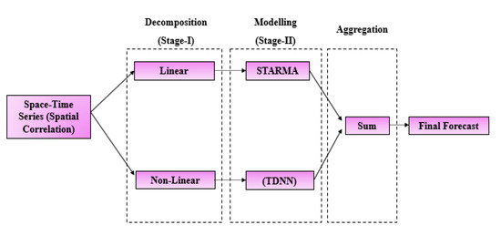
Figure 1.
General framework of two-stage spatiotemporal time series methodology.
Briefly, in the first phase, the space time series is modelled using the STARMA model and diagnostically tested using the multivariate Box-Pierce test. If this test is not significant, the procedure ends with the adjustment of the STARMA model and the transition to out-of-sample prediction (Figure 1). In the second stage, when the residuals are significant, the BDS test [38] is used to test for the nonlinearity of the residuals. If the residuals are found to be significant, the TDNN model is fitted to the residuals to obtain the fitted values (Figure 2). Finally, the TDNN fitted residuals are combined with the STARMA fitted values to obtain the final spatiotemporal forecast, where the final model can be expressed as:
where is the predicted residuals by TDNN model. The proposed two-stage approach is named as STARMA-II further in the study.
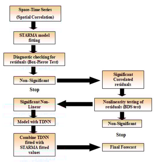
Figure 2.
Schematic representation of two-stage STARMA-II approach.
2.3. Testing of the STARMA-II Approach
The Diebold-Mariano (DM) test is used to determine the significant differences among the performance of two different models based on the residual values of two models [39]. The residuals of both models are and , the is defined as and the auto-covariance function is given as:
Finally, the DM test statistic can be expressed as:
where .
For testing of hypothesis, the null Hypothesis 0 (H0) and alternative Hypothesis 1 (H1) are defined as follows; null hypothesis: or the forecast accuracy is same for two methods and alternative hypothesis is , or the forecast accuracy is different for two methods.
2.4. Study Area Description and Input Data Used in Modelling
Geographical map of study area, the State of Andhra Pradesh (AP), India is shown in Figure 3. The selected geographical area comprises 13 intensively rice-producing districts (agroecosystems), making AP the seventh largest producer state with the second highest productivity (3539 kg/ha) of rice in India [40]. Rice yield data from these selected agroecosystems were collected for the period from 1991–1992 to 2019–2020 from the Directorate of Economics and Statistics, Andhra Pradesh, India. Rice yield data from 1991–1992 to 2015–2016 were used as training data set, while data from 2016–2017 to 2019–2020 were used as testing data set. Summary statistics of the rice yield spatiotemporal time series under consideration is given in Table S1.
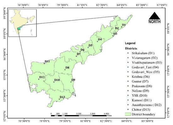
Figure 3.
Study area map of the examined area, Andhra Pradesh, India.
3. Results
3.1. Results of the ARIMA Model
Suitable candidate the ARIMA models were fitted to rice yield data, beginning by examining the stationarity of the data using Augmented Dickey-Fuller (ADF) test which revealed a positive trend over time, indicating that the time series under consideration is non-stationary in nature, hence first differencing was done to make the series stationary wherever necessary. The candidate ARIMA model chosen for different rice yield data series and their model estimation by using MLE is given in Table 1. After model fitting, diagnostic checking was done using Box-Pierce non-correlation test and residuals are found to be random.

Table 1.
Univariate ARIMA model fitting for rice yield (kg/ha) data across the examined area, Andhra Pradesh, India.
3.2. Creating Spatial Weight Matrix
As explained in the methodology section, defining of weight matrix is a key venture in building spatial weight matrix, and building of weight matrix is a modelers’ choice which in turn leads to model accuracy. In this study, it is assumed that the given area is influenced by its nearby neighbor, therefore, nearest neighbor to each district is identified by k nearest neighbor (knn) algorithm based on great circle distance formula by using longitude and latitude of the locations under consideration. The Great Circle Distance concept works based on the shortest distance between two points in a sphere along the surface of the sphere [13]. The coordinate matrix based on longitude and latitude is created to determine the nearest neighbor (Table S2) and based on the coordinate matrix nearest neighbor is determined as given in Table S3.
Once the nearest neighbor is determined, linear Karl Pearson’s correlation coefficient among the nearest neighbor is used to create the spatial weights. It is assumed that nearest neighbors are linearly correlated, hence are used as spatial weights. Zeroth order spatial weight matrix showed influence of rice yield on itself i.e., zeroth order neighbor (Table S4).
First order weight showed the first order weight matrix, which showed as to how a given district is influenced by its nearest neighbor. Second order weight matrix shows how a district is influenced by district next to immediate neighbor and so on in third order spatial weight matrix. Before determining the suitable spatial weight matrix, other uniform spatial weight matrix orders like first, second and third order spatial lags (Tables S5–S7) were tried and based on lowest BIC and highest log likelihood values, knn based spatial correlation weight matrix was chosen (Table 2). In knn based spatial correlation weight matrix, the nearest neighbor column, is assigned with correlation coefficient value (Table 3). The chosen, knn based spatial correlation weight matrix suffices multivariate Box-Pierce non-correlation test (Table 4).
Table 2.
Spatial lag determination for temporal AR 1 and MA1.
Table 3.
First order weight matrix based on linear correlation among nearest neighbor district.
Table 4.
STARMA model parameter estimation.
3.3. Results of the STARMA Model
In this section, classical space time autoregressive moving average model was fitted to spatiotemporal time series data on rice yield of the selected State. As like ARIMA model building, the STARMA model building also begins by testing presence of spatiotemporal correlation among the data series, the multivariate Box-Pierce non-Correlation test (Table 4) shows that data under consideration is spatiotemporally correlated and first differencing was done to make the series stationary.
Different space time autoregressive and space time moving average orders were tried and candidate STARMA () model was chosen based on Lowest AIC values.
where, and are the yield of a district i for year t and t − 1 respectively. Parameter specifications of fitted STARMA model is depicted in Table 5, which shows STAR and STMA parameters are significant, except the STAR parameter at first spatial and time lag is significant at level of significance.
Table 5.
BDS test statistics of STARMA (, , ) residuals.
3.4. Results of Proposed STARMA-II Approach
As explained in previous section, the STARMA (, , ) model was built for rice yield series in first stage, where by diagnostic checking of residuals it was found that probability value of multivariate Box-Pierce non-correlation test is significant. Consequently, this means that the residuals are not white-noise and the significant residuals contain some information. In the next, the BDS test confirmed that STARMA residuals were significant (Table 5), confirming the presence of nonlinearity in the STARMA residuals data set. The BDS test divides the data into two or more different dimensions (m) or parts, where it checks for nonlinearity individually.
In the second stage, the STARMA residuals were fitted with suitable TDNN models using feed forward network trained with back propagation algorithm by using sigmoidal activation function in input to hidden layer and liner identity function in hidden layer to output layer. The model specifications of the same are depicted in Table S8.
The fitted STARMA residuals with the TDNN model are combined or summed up with STARMA fitted values in both training and testing data set. After fitting the STARMA-II model, a diagnostic check was done using the Box-Pierce non-correlation test. Since the residuals were found to be random (p = 0.445), it was confirmed the model assumptions were satisfied. STARMA-II model performance in terms of MAPE in both training and testing set is depicted in Table 6.
Table 6.
Model performance in terms of MAPE in training and testing data sets.
4. Discussion
Rice is the staple food crop grown in all the districts of Andhra Pradesh providing food, fodder and employment security to farming communities in rural areas. The three districts, namely West Godavari, East Godavari and Krishna, are most important rice producing districts not only in Andhra Pradesh but also in the entire country. Forecasting of rice yield is used to provide an aid to decision-making and in planning the future effectively by formulating appropriate farm policies. This study was undertaken to predict the district wise rice yield by incorporating spatial dependence in the form of spatial weight matrices.
In STARMA modelling, the determination of spatial weights plays an important role in model building, which thus determines model accuracy, depending on the scope and limitations of the study. Uniform weight matrix or homogenous spatial weight matrix is the most ordinarily utilized spatial weight matrix in STARMA modelling [41]. However, the determination of the spatial weight matrix is contextual, and relatively subjective, i.e., it depends on the modeler’s choice. Thus, one should define the weight such that there is a significant spatial correlation between the adjacent. In this study, weight has been assigned based on Pearson’s linear correlation coefficient between nearest adjacent determined by k nearest neighbor (knn) algorithm [13]. Before deciding the appropriate spatial lags, different orders were tried and found that first uniform and knn based spatial weight matrices are yielding better BIC and log likelihood values. So, the knn based spatial weight matrix was chosen. The possible reasons for the same could be the farther distance among the districts. As distance among the places increases, it does not have strong influence on the neighboring places. A similar concept was explained in series of papers [15,16,21,22].
As ARIMA is the most popularly used model for forecasting time series data, we fitted the candidate ARIMA model to each district separately to predict rice yield. As explained in the methodology section, the model was fitted to both training and testing data sets. In testing data set, the ARIMA model yielded similar forecast values for all the four years which could be due to inability of ARIMA model to capture the spatiotemporal correlations among the neighboring districts. After ARIMA, the classical STARMA model was fitted to rice yield data of all the districts simultaneously in single model. After model fitting, diagnostic checking was done and it was found that residuals are spatially auto correlated in nature as chi-square test statistic was significant. This means that the fitted model is not properly explaining the complete information present in the data sets. Similar results were reported in prediction of mango and banana yield of Karnataka, India [29,31]. In addition to yield prediction, similar significance of the residuals was also observed in spatiotemporal modelling of rainfall data in West Bengal, India [14].
In general, nonlinearity or mixture of linear and nonlinear pattern in rice yield can be caused due to (i) different cropping management strategies (fertilization, pest and/or weed management, irrigation), (ii) agroecological (soil type, therein development, exposition) and/or (iii) climatological (air or soil temperature, air humidity, solar radiation, total precipitation) conditions [42,43,44]. Machine learning techniques have been used widely to develop crop-environmental models, and some of them highlighted the accuracy of some approaches (e.g., Random Forest regression) while attributing their superiority in handling data to multicollinearity and extracting nonlinear interactions [44]. Thus, agronomists, agro-meteorologists, crop data modelers and statisticians have attempted to quantitatively assess the effects of various biotic and/or abiotic impacts on crop (rice) development rate [44,45]. For instance, rice yield can be defined as a function of weed density and the duration of the weed-crop interference, where relation between weed density and crop yield is probably caused by the availability of solar radiation, phytonutrients, and/or water. The effects of the duration of weed-crop interference on crop yield exhibit similar nonlinearity with a characteristic upper asymptote in which increased duration no longer affects crop yield because yield components (e.g., grain number, size) have been determined. Furthermore, using a nonlinear model, it was confirmed that the optimal temperature for most rice cultivars is typically 27 ± 32 °C, while the developmental rate response of 24 rice cultivars to constant temperatures is typically nonlinear [45]. Availability of some critical inputs, such as mineral nitrogen, phosphorous, potassium and organic fertilizers, affect the rice production system [46,47], which in turn leads to unstable rice production over a period of time. Reference [48] studied trends and growth stability in rice production in Andhra Pradesh and identified that change in rice production could be due to instability in rice production cropping pattern, which in turn leads to fluctuations and nonlinearity in time series over a period of time. For instance, in Srikakulam, Godavari_East, Godavari_West and Prakasam districts, nonlinear pattern was more pronounced than in other districts. To overcome the modelling of above-mentioned mixture of linear and nonlinear pattern in spatiotemporal time series data, the two stage STARMA model was developed to capture the nonlinear spatiotemporal pattern in rice yield data. Similar modelling approaches were developed by the combination of two different models in different agricultural commodities like; maize yield [19], mango and banana yield prediction [29,31], coffee yield prediction [30] and rice yield prediction [32,33].
For example, in recent studies [32,33] rice yield data obtained from 1975 to 2013 in Aligarh district of Uttar Pradesh, India, were successfully predicted by rainfall, and like the proposed two-stage approach in this study, performed better in predicting rice yields compared to some single models. A major difference between previous studies [32,33], and here proposed STARMA-II model, is the inclusion of the effects of neighboring districts in the form of spatially-weighted matrices. Accordingly, STARMA-II was developed as a model for all 13 examined districts, whereas in previous studies [32,33] ARIMA model was applied to a single district level. The outperformance of STARMA over ARIMA approach has also been previously explained [15,16,21,22], highlighting that STARMA provides better prediction compared to ARIMA model when spatial correlation is present among neighboring districts.
Model performance in terms of MAPE in both training and testing set was carried out and the same is depicted in Table 6. It was observed that MAPE value of STARMA-II approach is less compared to ARIMA and STARMA model in both training and testing data set (Table 6) for all examined 13 districts. However, the above results exhibited only the observed differences between the models. Therefore, Diebold-Mariano test for significant predictive performance of each models were carried out and depicted in Table 7. It infers that proposed STARMA-II approach outperformed over both univariate ARIMA and classical STARMA model in both training and testing data set, with the performance hierarchy expressed as; STARMA-II > STARMA > ARIMA in both training and validation set.
Table 7.
Diebold-Mariano test for predictive accuracy of models under consideration.
The predicted rice yield of the proposed approach is closer to the actual yield values as compared to both the ARIMA and STARMA model (Table S9a,b). The possible reasons for outperformance of proposed two stage STARMA model could be due to its ability to capture both linear and nonlinear spatiotemporal patterns present in rice yield time series data. A study conducted by [49] with infectious disease data; [12] with temperature data; as well as [13] with freight flows data, reported that STARMA model yielded better forecast accuracy compared to univariate ARIMA model when spatial dependence exists in the data sets.
5. Conclusions
The autoregressive and moving average components of time series slacked in both space and time are the most useful model for modelling and forecasting spatiotemporal time series data. As space-time ARIMA is a linear model, which is unable to characterize the nonlinear spatiotemporal relationships and linear approximations to complex nonlinear spatiotemporal pattern, it is not always satisfactory. Alternatively, TDNN is the most promising machine learning algorithm to model the nonlinear pattern in time series data, while in combination with STARMA it is more promising in its linear and nonlinear modelling task, to amalgamate the merits of both algorithms to model the mixed spatiotemporal series.
Thus, two-stage STARMA-II approach has been proposed to predict the annual rice yield data across the intensive rice agroecosystems of Andhra Pradesh, India. It was confirmed that the STARMA-II approach outperformed the classical models in all examined districts, while DM test confirmed that the performance of the STARMA-II is significantly different with respect to both ARIMA and classical STARMA models. In future studies, some other (a)biotic factors important for yield performance of rice will also be included and their importance evaluated. Finally, different AI techniques are expected to be put into use to model the non-linear spatiotemporal time series for varying autoregressive and space time moving average orders, and their applications can be extended to various real-time datasets in advanced agroecosystem management, as well in more sustainable food supply-demand planning at (inter)national scales.
Supplementary Materials
The following are available online at https://www.mdpi.com/article/10.3390/agronomy11122502/s1, Table S1: Descriptive statistics of rice yield (kg/ha) data across the examined area, Andhra Pradesh, India, Table S2. Coordinate matrix for districts of A.P. India, Table S3: Nearest neighbours for each districts of A.P. India, Table S4: Zero order weight matrix among examined districts, Table S5: First order uniform spatial weight matrix, Table S6: Second order uniform spatial weight matrix, Table S7: Third order uniform spatial weight matrix, Table S8. TDNN model parameter specifications for STARMA (, ,) residuals series, Table S9a: Out of sample forecasts obtained by different methods, Table S9b: Out of sample forecasts obtained by different methods.
Author Contributions
Conceptualization, S.R.; Data curation, S.R.; Formal analysis, S.R., A.S. and R.P.; Investigation, S.R.; Methodology, S.R., A.S. and G.O.; Resources, R.M.S.; Software, S.R., A.S. and R.P.; Supervision, G.O., C.G. and D.V.K.N.R.; Visualization, G.O., C.G., M.S.A., D.V.K.N.R., N.B., P.S., A.K.S., S.N.M., A.W., P.J., B.P., P.M. and R.M.S.; Writing—original draft, S.R.; Writing—review & editing, G.O., C.G., M.S.A., D.V.K.N.R., N.B., P.S., A.K.S., S.N.M., A.W., P.J., B.P., P.M. and R.M.S. All authors have read and agreed to the published version of the manuscript.
Funding
This research received no external funding.
Institutional Review Board Statement
Article approved for submission. Ref. No. IIRR/DIR/PD/PMEC/2021-22/Res.Paper/427dt. 24 September 2021.
Informed Consent Statement
Not applicable.
Data Availability Statement
The data presented in this study are collected from reports of agricultural statistics at glance published by Department of Economics and Statistics, Andhra Pradesh, India.
Acknowledgments
The authors would like to thank Indian council of Agricultural Research—Indian Institute of Rice Research, Hyderabad, India for their support in this research work. Also, we are grateful to anonymous reviewers on numerous comments and suggestions which improved the final text.
Conflicts of Interest
The authors declare no conflict of interest.
References
- Ondrasek, G.; Rengel, Z. Environmental Salinization Processes: Detection, implications & solutions. Sci. Total Environ. 2021, 754, 142432. [Google Scholar] [CrossRef]
- Ali, S.; Ghosh, B.C.; Osmani, A.G.; Hossain, E.; Fogarassy, C. Farmers’ Climate Change Adaptation Strategies for Reducing the Risk of Rice Production: Evidence from Rajshahi District in Bangladesh. Agronomy 2021, 11, 600. [Google Scholar] [CrossRef]
- Food and Agriculture Organization of the United Nations. FAOSTAT Statistical Database; FAO: Rome, Italy, 2021; Available online: https://www.fao.org/faostat/en/#data (accessed on 21 September 2021).
- Agricultural Statistics at Glance; Ministry of Agriculture & Farmers Welfare Department of Agriculture; Cooperation & Farmers Welfare Directorate of Economics & Statistics; Government of India. 2020. Available online: https://eands.dacnet.nic.in/PDF/At%20a%20Glance%202019%20Eng.pdf (accessed on 21 September 2021).
- Romić, D.; Castrignanò, A.; Romić, M.; Buttafuoco, G.; Bubalo Kovačić, M.; Ondrašek, G.; Zovko, M. Modelling Spatial and Temporal Variability of Water Quality from Different Monitoring Stations using Mixed Effects Model Theory. Sci. Total Environ. 2020, 704, 135875. [Google Scholar] [CrossRef]
- Sein, Z.M.M.; Zhi, X.; Ogou, F.K.; Nooni, I.K.; Lim Kam Sian, K.T.C.; Gnitou, G.T. Spatio-Temporal Analysis of Drought Variability in Myanmar Based on the Standardized Precipitation Evapotranspiration Index (SPEI) and Its Impact on Crop Production. Agronomy 2021, 11, 1691. [Google Scholar] [CrossRef]
- Marino, S.; Alvino, A. Detection of Spatial and Temporal Variability of Wheat Cultivars by High-Resolution Vegetation Indices. Agronomy 2019, 9, 226. [Google Scholar] [CrossRef] [Green Version]
- Giacinto, V.D. A Generalized Space—Time ARMA Model with an Application to Regional Unemployment Analysis in Italy. Int. Reg. Sci. Rev. 2006, 29, 159–198. [Google Scholar] [CrossRef]
- Zhao, P.; Zhou, Y.; Li, F.; Ling, X.; Deng, N.; Peng, S.; Man, J. The Adaptability of APSIM-Wheat Model in the Middle and Lower Reaches of the Yangtze River Plain of China: A Case Study of Winter Wheat in Hubei Province. Agronomy 2020, 10, 981. [Google Scholar] [CrossRef]
- White, M.A.; Diffenbaugh, N.S.; Jones, G.V.; Pal, J.S.; Giorgi, F. Extreme Heat Reduces and Shifts United States Premium Wine Production in the 21st century. Proc. Natl. Acad. Sci. USA 2006, 103, 11217–11222. [Google Scholar] [CrossRef] [PubMed] [Green Version]
- Neuman, K.; Verburg, P.H.; Stehfest, E.; Muller, C. The yield Gap of Global Grain Production: A Spatial Analysis. Agric. Syst. 2010, 103, 316–326. [Google Scholar] [CrossRef]
- Rathod, S.; Gurung, B.; Singh, K.N.; Ray, M. An Improved Space-Time Autoregressive Moving Average (STARMA) Model for Modelling and Forecasting of Spatio-Temporal Time-Series Data. J. Ind. Soc. Agric. Stat. 2018, 72, 239–253. [Google Scholar]
- Sahu, P.K.; Padhi, A.; Patil, G.R.; Mahesh, G.; Sarkar, A.K. Spatial Temporal Analysis of Freight Flow through Indian Major Seaport System. Asian J. Shipp. Logist. 2019, 35, 77–85. [Google Scholar] [CrossRef]
- Saha, A.; Singh, K.N.; Ray, M.; Kumar, S.; Rathod, S. A New Approach for Spatio-Temporal Modelling and Forecasting based on Fuzzy Techniques in conjunction with K-means clustering. J. Ind. Soc. Agric. Stat. 2019, 73, 111–120. [Google Scholar]
- Pfeifer, P.E.; Deutsch, S.J. Seasonal Space-Time ARIMA modelling. Geogr. Anal. 1981, 13, 117–133. [Google Scholar] [CrossRef]
- Pfeifer, P.E.; Deutsch, S.J. Space-Time ARMA Modelling with contemporaneously correlated innovations. Technometrics 1981, 23, 401–409. [Google Scholar]
- Zhao, Y.; Ge, L.; Zhou, Y.; Sun, Z.; Zheng, E.; Wang, X.; Huang, Y.; Cheng, H. A new Seasonal Difference Space-Time Autoregressive Integrated Moving Average (SD-STARIMA) model and spatiotemporal trend prediction analysis for Hemorrhagic Fever with Renal Syndrome (HFRS). PLoS ONE 2018, 13, e0207518. [Google Scholar] [CrossRef] [PubMed]
- Box, G.E.P.; Jenkins, G. Time series analysis. In Forecasting and Control; Holden-Day: San Francisco, CA, USA, 1970. [Google Scholar]
- Rathod, S.; Singh, K.N.; Arya, P.; Ray, M.; Mukherjee, A.; Sinha, K.; Kumar, P.; Shekhawat, R.S. Forecasting maize yield using ARIMA-Genetic Algorithm approach. J. Outlook Agric. 2017, 46, 265–271. [Google Scholar] [CrossRef]
- Pfeifer, P.E.; Deutsch, S.J. A Comparison of Estimation Procedures for the Parameters of the STAR Model. Commun. Stat. Simul. Comput. 1980, 9, 255–270. [Google Scholar] [CrossRef]
- Pfeifer, P.E.; Deutsch, S.J. A Three-Stage Iterative Procedure for Space-Time Modeling. Technometrics 1980, 22, 35–47. [Google Scholar] [CrossRef]
- Pfeifer, P.E.; Deutsch, S.J. Identification and Interpretation of First-Order Space-Time ARMA Models. Technometrics 1980, 22, 397–403. [Google Scholar] [CrossRef]
- Pfeifer, P.E.; Deutsch, S.J. Independence and Sphericity Tests for the residuals of Space Time ARIMA Models. Commun. Stat. Simul. Comput. 1980, 9, 533–549. [Google Scholar] [CrossRef]
- Pfeifer, P.E.; Deutsch, S.J. Variance of the Sample-Time Autocorrelation Function of Contemporaneously Correlated Variables. SIAM J. Appl. Math. Ser. A 1981, 40, 133–136. [Google Scholar] [CrossRef]
- Rathod, S.; Singh, K.N.; Patil, S.G.; Naik, R.H.; Ray, M.; Meena, V.S. Modelling and Forecasting of Oilseed Production of India through Artificial Intelligence Techniques. Indian J. Agric. Sci. 2018, 88, 22–27. [Google Scholar]
- Chitikela, G.; Admala, M.; Ramalingareddy, V.K.; Bandumula, N.; Ondrasek, G.; Sundaram, R.M.; Rathod, S. Artificial-Intelligence-Based Time-Series Intervention Models to Assess the Impact of the COVID-19 Pandemic on Tomato Supply and Prices in Hyderabad, India. Agronomy 2021, 11, 1878. [Google Scholar] [CrossRef]
- Zhang, G.P. Time-Series Forecasting using a Hybrid ARIMA and Neural Network Model. Neurocomputing 2003, 50, 159–175. [Google Scholar] [CrossRef]
- Jha, G.K.; Girish, K.J.; Sinha, K. Time-Delay Neural Networks for Time Series Prediction: An Application to the Monthly Wholesale Price of Oilseeds in India. Neural. Comput. Appl. 2014, 24, 563–571. [Google Scholar] [CrossRef]
- Rathod, S.; Mishra, G.C.; Singh, K.N. Hybrid Time Series Models for Forecasting Banana Production in Karnataka State, India. J. Ind. Soc. Agric. Stat. 2017, 71, 193–200. [Google Scholar]
- Naveena, K.; Singh, S.; Rathod, S.; Singh, A. Hybrid Time Series Modelling for Forecasting the Price of Washed Coffee (Arabica Plantation Coffee) in India. Int. J. Agric. Sci. 2017, 9, 4004–4007. [Google Scholar]
- Rathod, S.; Mishra, G.C. Statistical Models for Forecasting Mango and Banana Yield of Karnataka, India. J. Agri. Sci. Technol. 2018, 20, 803–816. [Google Scholar]
- Alam, W.; Ray, M.; Kumar, R.R.; Sinha, K.S.; Singh, K.N. Improved ARIMAX modal based on ANN and SVM approaches for forecasting rice yield using weather variables. Indian J. Agric. Sci. 2018, 88, 1909–1913. [Google Scholar]
- Alam, W.; Sinha, K.; Kumar, R.R.; Ray, M.; Rathod, S.; Singh, K.N.; Arya, P. Hybrid linear time series approach for long term forecasting of crop yield. Indian J. Agric. Sci. 2018, 88, 1275–1279. [Google Scholar]
- Cheng, T.; Wang, J. Application of a Dynamic Recurrent Neural Network in Spatio-Temporal Forecasting in Information Fusion and Geographic Information Systems Germany; Springer: Berlin, Germany, 2007; pp. 173–186. [Google Scholar]
- Saputro, D.R.S.; Putri, I.M.; Noor, N.H.; Widyaningsih, P. Generalized Space Time Autoregressive (gstar)-Artificial Neural Network (ANN) Model with Multilayer Feedforward Networks Architecture. IOP Conf. Ser. Earth Environ. Sci. 2019, 243, 012039. [Google Scholar] [CrossRef]
- Konduri, V.S.; Vandal, T.J.; Ganguly, S.; Ganguly, A.R. Data Science for Weather Impacts on Crop Yield. Front. Sustain. Food Syst. 2020, 4, 52. [Google Scholar] [CrossRef]
- Saha, A.; Singh, K.N.; Ray, M.; Rathod, S. A hybrid spatio-temporal modelling: An application to space-time rainfall forecasting. Theor. Appl. Climatol. 2020, 142, 1271–1282. [Google Scholar] [CrossRef]
- Brock, W.; Scheinkman, J.A.; Dechert, W.D.; LeBaron, B. A Test for Independence Based on the Correlation Dimension. Eco. Rev. 1996, 15, 197–235. [Google Scholar] [CrossRef]
- Diebold, F.X.; Mariano, R.S. Comparing predictive accuracy. J. Bus. Econ. Stat. 1995, 13, 253–263. [Google Scholar]
- Agricultural Statistics at Glance; Directorate of Economics and Statistics; Government of Andhra Pradesh. 2020. Available online: https://foodprocessingindia.gov.in/uploads/publication/Agricultural-statistics-at-a-Glance-2020.pdf (accessed on 29 January 2021).
- Subba, R.T.; Antunes, A. 2003 Spatio-Temporal Modelling of Temperature Time Series: A Comparative Study. In Time Series Analysis and Applications to Geophysical Systems; Schonberg, F.P., Brillinger, D.R., Robinson, E.A., Eds.; IMA Publications/Springer: New York, NY, USA, 2003; pp. 123–150. [Google Scholar]
- Yin, X.; Kropff, M.J.; McLeare, G.; Visperas, R.M. A nonlinear model for crop development as a function of temperature. Agric. For. Meteorol. 1995, 77, 1–16. [Google Scholar] [CrossRef] [Green Version]
- Yin, X.; Kropff, M.J.; Ellis, R.H. Rice flowering in response to diurnal temperature amplitude. Field Crop. Rese. 1996, 48, 1–9. [Google Scholar] [CrossRef]
- Piyal Ekanayake, P.; Rankothge, W.; Weliwatta, R. Machine Learning Modelling of the Relationship between Weather and Paddy Yield in Sri Lanka. J. Math. 2021, 2021, 9941899. [Google Scholar] [CrossRef]
- Yin, X.; Kropff, M.J.; Goudriaan, J. Differential Effects of Day and Night Temperature on Development to Flowering in Rice. Anna Bota 1996, 77, 203–213. [Google Scholar] [CrossRef] [Green Version]
- Alam, M.N.; Effendy. Identifying Factors Influencing Production and Rice Farming Income with Approach of Path Analysis. Am. J. Agric. Biol. Sci. 2017, 12, 39–43. [Google Scholar] [CrossRef]
- Prasanna, P.A.L.; Kumar, S.; Singh, A. Rice Production in India—Implications of Land Inequity and Market Imperfections. Agri. Econ. Res. Rev. 2009, 22, 431–442. [Google Scholar]
- Sunandini, G.P.; Paul, K.S.R.; Irugu, S.D. Analysis of Trends, Growth and Instability in Rice Production in Andhra Pradesh. Curr. J. Appl. Sci. Technol. 2020, 39, 40–46. [Google Scholar] [CrossRef]
- Lee, C.Y. Space-Time Modelling and Application to Emerging Infectious Diseases. Ph.D. Thesis, Michigan State University, East Lansing, MI, USA, 2005. [Google Scholar]
Publisher’s Note: MDPI stays neutral with regard to jurisdictional claims in published maps and institutional affiliations. |
© 2021 by the authors. Licensee MDPI, Basel, Switzerland. This article is an open access article distributed under the terms and conditions of the Creative Commons Attribution (CC BY) license (https://creativecommons.org/licenses/by/4.0/).