Article

Machine Learning Approach to Simulate Soil CO2 Fluxes under Cropping Systems

1
Department of Biosystems and Agricultural Engineering, University of Kentucky, 128 CE Barnhart Building, Lexington, KY 40546, USA
2
Environmental Studies Program, Voinovich School of Leadership and Public Service, Ohio University, The Ridges, Building 22, Athens, OH 45701, USA
3
Department of Environmental and Plant Biology, Ohio University, Athens, OH 45701, USA
*
Authors to whom correspondence should be addressed.
Agronomy 2022, 12(1), 197; https://doi.org/10.3390/agronomy12010197
Submission received: 8 December 2021 / Revised: 6 January 2022 / Accepted: 10 January 2022 / Published: 14 January 2022

Abstract

:
With the growing number of datasets to describe greenhouse gas (GHG) emissions, there is an opportunity to develop novel predictive models that require neither the expense nor time required to make direct field measurements. This study evaluates the potential for machine learning (ML) approaches to predict soil GHG emissions without the biogeochemical expertise that is required to use many current models for simulating soil GHGs. There are ample data from field measurements now publicly available to test new modeling approaches. The objective of this paper was to develop and evaluate machine learning (ML) models using field data (soil temperature, soil moisture, soil classification, crop type, fertilization type, and air temperature) available in the Greenhouse gas Reduction through Agricultural Carbon Enhancement network (GRACEnet) database to simulate soil CO2 fluxes with different fertilization methods. Four machine learning algorithms—K nearest neighbor regression (KNN), support vector regression (SVR), random forest (RF) regression, and gradient boosted (GB) regression—were used to develop the models. The GB regression model outperformed all the other models on the training dataset with R2 = 0.88, MAE = 2177.89 g C ha−1 day−1, and RMSE 4405.43 g C ha−1 day−1. However, the RF and GB regression models both performed optimally on the unseen test dataset with R2 = 0.82. Machine learning tools were useful for developing predictors based on soil classification, soil temperature and air temperature when a large database like GRACEnet is available, but these were not highly predictive variables in correlation analysis. This study demonstrates the suitability of using tree-based ML algorithms for predictive modeling of CO2 fluxes, but no biogeochemical processes can be described with such models.

1. Introduction

According to the U.S Environmental Protection Agency, CO2 is the primary anthropogenic greenhouse gas (GHG) emitted in the US, with a 30% atmospheric increase since the pre-industrial era [1], and it accounted for 80% of the total GHG emissions into the atmosphere in 2019 [2]. Though the greatest sources of CO2 in the US are transportation, electricity and the industrial sectors [2], agriculture also accounts for substantial CO2 emissions. Emissions of CO2 from agriculture include respiratory fluxes from root growth and turnover, microbial respiration, aboveground plant respiration [3] and also the stimulation of these fluxes that occur from the application of nitrogen fertilizers [4]. Current estimated soil carbon is about 2700 gigatons (1 gigaton = 1 billion metric tons) worldwide with two-thirds of that carbon in organic form [5,6], which is three times the amount of carbon currently in the atmosphere [7]. As a result, an increase of a few percentage points in soil carbon uptake affects the CO2 entering the atmosphere [6], decreasing the amount of GHG emissions. Estimating soil CO2 emissions is thus essential for understanding the feedbacks between climate changes and terrestrial ecosystems [8]. A major challenge however is that direct measurement of CO2 fluxes from soil can be costly, time-consuming, and require some level of expertise, making it challenging to quantify the CO2 emissions emanating from different crop management systems, especially where soil conditions are highly variable.
Emissions of CO2 from soil result primarily from microbial activity, root respiration, chemical decay processes, and heterotrophic respiration of soil microorganisms [3]. Soil moisture, soil temperature, land cover, vegetation, and nutrients all play a role in soil CO2 emission [3]. There are various standardized methods for measuring CO2 fluxes from soils, including the chamber methods (close static chamber method, dynamic static chamber method or open chamber methods), micrometeorological methods such as the eddy covariance [3], and the soil CO2 gradient system [9]. However, various weaknesses have been identified with these methods for quantifying CO2 soil fluxes. For example, Heinemeyer & McNamara [10] argue that the closed static chamber approach takes a long time to manually sample, which can underestimate the calculated fluxes due to asymptotic increase in headspace CO2 concentrations. Although the soil CO2 gradient system has some advantages over the chamber-based methods, Liang et al. [9] argue that the sensors used for measuring CO2 flux are not very accurate and can be damaged by the soil microenvironment. Despite the weaknesses identified with in situ measurements of soil GHG fluxes, all modeling approaches rely on data generated from field and laboratory studies to describe complex physical, biological, and chemical processes occurring in the soil. Thus, the performance of modeling studies depends on the continued collection of complete and quality observed data to improve results from modeling approaches [11].

1.1. Review of Previous Studies

Biogeochemical models are other alternatives to the traditional direct measurement of CO2 which have been developed over the years to predict GHGs. Some of these biogeochemical models include the Denitrification Decomposition model (DNDC) model proposed by Li et al. [12], the SOILCO2 model by Herbst et al. [13], the DAYCENT model [14,15], and the Root Zone Water Quality Model (RZWQM2) [16]. Although biogeochemical and process-based models have been successful at estimating soil CO2 fluxes, they possess certain limitations; for example, in the DAYCENT model, Del Grosso et al. [14] explains that errors can emanate from uncertainty in model drivers and imperfections in model parameterizations. In addition, complex models such as DAYCENT and RZWQM2 often require experienced users with agro-ecological expertise to implement pre-procedures, model calibration and validation [17] which may limit their wide usage.
An alternative to direct measurement and biogeochemical models for predicting soil GHG fluxes is to use models based on machine learning. The development of big data technologies and high-performance computing has propelled machine learning (ML) as a tool to create new opportunities to reveal, quantify and understand data-intensive processes in agriculture [18]. Machine learning models are not meant to replace biogeochemical models and direct measurement, but are meant to complement these existing methods, especially when direct measurement is difficult. Machine learning (ML) algorithms utilize pattern recognition to describe relationships between input parameters and output parameters by “learning” characteristics of the relationships after training a given dataset [19]. ML models require a large amount of data to be able to learn intricate relationships such that when new data is introduced to the model, it can still generate accurate predictions. ML models seek to establish statistical relationships through iterative multivariate analysis to maximize correlations between input variables and an output variable in a given set of data [20]. Table 1 summarizes previous studies that applied various ML techniques to predict soil GHG fluxes.

1.2. Rationale for ML Study of Soil CO2

Soil GHG emissions (i.e., CO2) in agricultural soils are influenced by the soil type, pH, carbon content, tillage practices, soil temperature, moisture content [27], the type of fertilizer applied [28], and the cropping system [29]. In this study, our goal was to determine the plausibility of using basic soil physical properties (soil temperature, soil moisture, soil type), air temperature, cropping system, and the type of fertilization as input variables to estimate CO2 fluxes. A previous study by the authors [28] revealed that application of a novel organic based soil amendment (hydrochar) reduced soil CO2 fluxes by 34% compared to inorganic fertilizer (urea) and these CO2 fluxes were correlated with soil temperature. Although the study [28] was only conducted on one cropping system (a 6-year-old miscanthus stand), previous studies have shown that switching from conventional annual crops such as corn, to perennial bioenergy crops such as miscanthus, could significantly reduce GHG fluxes due to the limited fertilizer application needed and the increased carbon sequestration [30,31]. Understanding the consequence of different fertilizer uses in a variety of cropping systems is thus important for agricultural development that reduces CO2 emissions from soils. Therefore, the goal of this study was to determine if large datasets from many studies and cropping systems can be used to train ML models to estimate CO2 fluxes with minimal predictors.

1.3. Purpose of Study

The objective of this study was to develop and evaluate ML-based models using data (soil temperature, soil moisture, soil classification, crop type, fertilization type, and air temperature) available in the Greenhouse Gas Reduction through Agricultural Carbon Enhancement network (GRACEnet) database to predict yearly soil CO2 fluxes under different management systems. We hypothesized that fertilizer type could be used as a predictor of soil CO2 fluxes in ML models. Because ML algorithms do not evaluate predictive power of individual variables statistically, we also assessed the input variables used to develop the models by applying correlation analysis to determine which variables were most strongly correlated with changes in soil CO2 emissions. Multiple ML algorithms were used to develop the models including support vector regression (SVR), random forest regression (RF), K-nearest neighbor regression (KNN), and gradient boosted regression (GB). To the best of our knowledge, no study has utilized the GRACEnet database to develop ML models to predict CO2 soil fluxes and this study therefore evaluates a new approach.

2. Materials and Methods

2.1. Description of the Database

The data used in this modeling study was derived from the GRACEnet database. The main purpose of the GRACEnet database is to aggregate information from many studies so that methods for quantifying GHG emissions and other environmental impacts of cropped and grazed systems can be developed, and to provide scientific evidence for carbon trading programs that can help reduce GHG emissions [32]. GRACEnet consists of a large network of researchers who conduct field experiments that quantify soil C and/or GHG emission data under three scenarios: scenario one is a “business as usual” management system, scenario two is a system that maximizes soil carbon sequestration, and scenario three is a system that minimizes net GHG fluxes from soils [33]. The database contains GHG data from 169,858 individual GHG measurements from 25 different field sites with associated background descriptors about the location, weather, and plot designations [33]. Even though the original database consisted of 34 tables, with each table containing data that may be needed based on a specific research hypothesis, we selected the table that contained the CO2 emissions measurements. The GHG emissions measurement data originally consisted of 53 columns. The columns contained descriptive information such as the start and end dates of the respective studies, crop rotation, tillage description, cover cropping, and irrigation. Although several of these agricultural parameters found in the GRACEnet database could influence CO2 fluxes, we opted for fewer categorical variables and more continuous variables because ML regression algorithms can be biased, especially when categorical variables have several sub-levels. The categorical variables of greatest interest for this study are the fertilizer amendment class, soil classification and crop type. Thus, six variables (air temperature, soil temperature, soil moisture, fertilizer amendment class, soil classification, crop) and one response variable (CO2 fluxes) were selected for the analysis. These variables have known effects on soil CO2 emissions [3,17,28] but have not been tested in ML methods as predictors for estimating CO2 fluxes. The crop type category that represented the land use or cropping system in the different sites contained a total of 24 different categories (e.g., corn, pasture, rangeland, miscanthus, fallow, etc.), from which a subset was selected during preprocessing. The fertilizer amendment class refers to the type of fertilizer (synthetic, organic, combination of synthetic and organic, or none) applied to a particular plot/site. The soil classification variable refers to the National Cooperative Soil Survey soil taxonomic classification of the soils. These included the following soil types: (1) Fine-mixed, semiactive, mesic Typic Hapludalfs, (2) Fine-silty, mixed, active, mesic Typic Paleudalfs, (3) Coarse-silty, mixed, mesic Durixerollic Calciorthods, (4) Fine-loamy, mixed, superactive, mesic Aridic Haplustalfs, frigid Typic Argiustoll, (5) Fine-loamy, mixed, superactive, mesic Ustic Haplocambids, (6) Tomek fine, smectitic, mesic Pachic Argiudolls, Filbert fine, smectitic, mesic Vertic Argialbolls, (7) Clayey, illitic, mesic Typic Hapludults, and (8) Fine-silty, mixed, superactive, rigid Typic and Pachic Haplustolls).

2.2. Preprocessing

Preprocessing is one of the most important steps in ML modeling because data that contain extraneous and irrelevant information produce less accurate results [34]. Data preprocessing steps can vary depending on the project but common steps in preprocessing involve data cleaning, normalization, transformation, and feature selection [34]. As with all real-world big databases, the GRACEnet database had thousands of missing data points that required verification or deletion. According to Lakshminarayan et al. [35], one method of dealing with missing data is by ignoring and discarding incomplete records and attributes, especially when missing data form a smaller proportion of the data and using complete data does not lead to biases in inferences. The first step of preprocessing in this study was to identify and eliminate missing data. The total number of samples/rows were 126,520 and the missing data accounted for about 36% of the total number. Thus, the remaining number of observations/rows used for the next preprocessing stage was 80,806. There were a total of 24 different types of crops in the categorical variable “crop,” but only five were used in this study and these included corn, switchgrass, miscanthus, pasture, and fallow lands. After dropping observations (rows) containing crops that were not relevant to this study, the total number of rows were drastically reduced to 7863. Model training is a computationally expensive process and so efforts were made to ensure only relevant samples were used for the modeling. The variables “crop”, “fertilizer amendment class” and “soil classification” in the subset dataset were converted from categorical variables to numeric category variables (i.e., dummy variables).

2.3. Machine Learning Implementation

Prior to implementing the machine learning algorithms, we determined the optimum number of input variables that significantly explained the most variation in the output variable (CO2 flux) using Pearson correlation analysis and step-forward feature selection [36]. Step-forward feature selection is a family of greedy search algorithms that reduces the number of initial variables to obtain an optimal number of variables that predict an output variable [37]. The algorithm starts with zero input variables, and then finds one input variable that maximizes a cross-validated evaluation criteria after training using an estimator (e.g., random forest regressor). The algorithm then sequentially adds the remaining input variables and repeats the procedure until a predetermined number of features are found. In step-forward feature selection, the algorithm evaluates all predictors individually and selects the predictors that give the highest value according to a pre-set evaluation criteria (R2) [37]. The algorithm then evaluates all possible combinations of the selected predictors to produce the best combination of predictors.
Four supervised regression ML algorithms (support vector regression (SVR), random forest regression (RF), K-nearest neighbor regression (KNN), and gradient boosted regression (GB) were used to develop models to predict soil CO2 fluxes. The models were programmed using Python (version 3.8.5). We used the Scikit-learn module, a Python module which integrates both supervised and unsupervised learning ML algorithms [38]. Supervised ML algorithms are those algorithms that need labeled (measured/known) training datasets to predict an output variable, whereas unsupervised ML algorithms do not need labeled data to predict the output variable [39].
A summary of the steps that were followed in implementing the ML algorithms are shown in Figure 1. Relevant information from the GRACEnet database was cleaned and preprocessed, and relevant features/predictors selected. After the preprocessing and feature selection steps, the input variables were scaled. The most common methods of scaling input variables are by normalization or standardization. In normalization, the input variables are scaled to have a range of 0 to 1 by subtracting the minimum value and dividing by the range between the maximum and minimum value of an input variable [40]. Standardization is achieved by subtracting the mean of an input variable from each value and dividing the result by the standard deviation [40]. We chose to normalize the input variables because normalization allows variables with different units to be equally represented in the ML framework.
The data were randomly split into a training set (80%), which had 6290 CO2 measurements used to build the models, and a test set (20%) of 1573 CO2 measurements, which were used to validate/test the models accuracy. When training models using ML algorithms, it is important to use the optimum hyperparameters of the specific algorithm to achieve the best model performance. The hyperparameters of an algorithm are the parameters that can be configured to minimize the loss function of the model which increases accuracy in the models being developed [41]. Thus, after training the models, optimum hyperparameters were found using the “GridSearchCV” function in Scikit-learn. The GridSearchCV function was used because it works by combining all given hyperparameter configurations to obtain the best set of hyperparameters that give the best performance within a user chosen configuration space [41]. The optimum hyperparameters were then used to retrain the models and final predictions of the accuracy of the models were made using the unseen test dataset reserved.
Model predictions of CO2 were compared to measured CO2 emissions using statistical performance measurements i.e., Mean Absolute Error (MAE), Root Mean Squared Error (RMSE), and R-Squared.

2.4. Computational Software

The computational software in this study was written with Python (programming language) (version 3.8.5) [42]. The advantage of using Python is its free and open-source nature, which means it is regularly checked and bugs fixed when reported to the programmers. For easy understanding, the code for this study was written in Jupyter Notebook [43]. Jupyter Notebook is an open-source web application that allows for easy creation and sharing of code, data cleaning, machine learning modeling and data visualization. To implement the four ML models, a series of algorithms (KNeighborsRegressor, RandomForestRegressor, SVR, and GradientBoostingRegressor) were downloaded onto the Jupyter Notebook environment from Scikit-learn (a Python module which integrates a series of ML algorithms) [38]. Data visualization was undertaken using matplotlib and seaborn, which are libraries available in Python. Forward feature selection was implemented using the SequentialFeatureSelector algorithm which was used to select the optimum number of features/variables prior to model development. The SequentialFeatureSelector algorithm can be found in MLxtend (a library that implements a variety of ML algorithms) [44]. Finally, to determine the most important variables in the best performing models, the “permutation importance” function in Scikit-learn was used to calculate the feature importance of the estimators in this study [38].

2.5. Machine Learning Techniques

Machine learning (ML) algorithms are generally grouped into supervised ML, unsupervised ML, semi-supervised learning, reinforcement, transduction, and learning to learn ML algorithms [45]. Supervised ML algorithms are those algorithms that generate a function that maps inputs to desired output from externally supplied labels (a data consisting training observations where each observation has a pair consisting of a predictor and a desired output variable) to make predictions on future observations [45,46]. Supervised ML algorithms are commonly used to predict GHG fluxes. Supervised ML is especially helpful when the output to be predicted is a continuous variable, e.g., CO2 fluxes. Although the supervised ML algorithms used in this study all aim to achieve a similar goal, to predict the CO2 fluxes given certain influential predictors, their operating principles differ, with different levels of complexity depending on the number of hyperparameters in the algorithm (Table 2). The size of the training dataset, the range of the training dataset compared to the testing dataset, the quality, and completeness of the overall dataset will determine which algorithm will yield the best performance. Operating principles, advantages, and disadvantages of the machine learning techniques used in this study are summarized in Table 2.

3. Results and Discussion

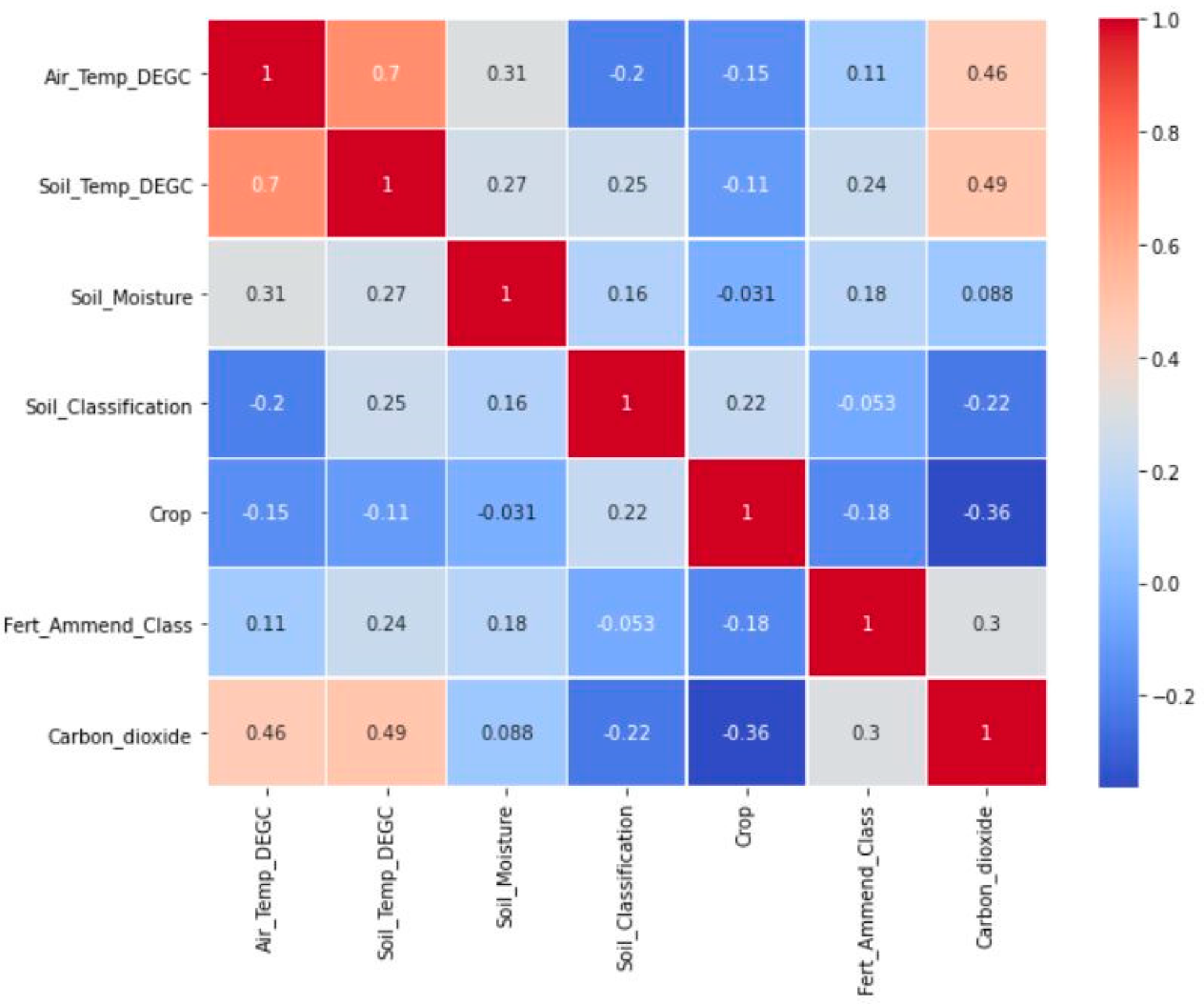
3.1. Feature Selection

Prior to implementing the machine learning algorithms, the relationships between the input variables and CO2 fluxes were analyzed to determine which input variables influenced the output variable the most. The coefficient of correlation (r) for all the predictors with the output variable was significant, with α = 0.05. The input parameters that were tested were air temperature, soil temperature, soil moisture, soil classification, crop, and fertilization amendment class. Four predictors (air temperature, soil temperature, crop, and fertilization amendment class) were moderately correlated with CO2 flux (r = 0.46, 0.49, 0.36, and 0.3, respectively), whereas soil moisture and soil classification had low correlations (r = 0.09 and 0.22, respectively) with CO2 flux. The moderate correlation of air temperature and soil temperature indicates their influence on CO2 fluxes is consistent with other studies [3,17].
Forward feature selection was implemented to choose the most important features for developing the models. Prior to implementing forward feature selection, we tested for multicollinearity between the predictors and none of the predictors were correlated to the other. The threshold to determine if two variables were correlated was that the absolute value of the correlation coefficient should exceed 0.8. In forward feature selection, predictors are added to a model one at a time. The algorithm first starts with the evaluation of each individual predictors, and selects the predictor which results in the best performing model as the starting predictor, according to a predetermined evaluation criteria (R2) [37].
In the next step, the algorithm starts with the best predictor and combines it with the remaining predictors to select the best pair of predictors. The algorithm continues adding predictors until a stopping criterion is reached and, in our study, until a predetermined number of predictors is selected. In our study, we tested cases with 1, 2, 3, 4, 5, and 6 predictors. Random forest was shown to be the best algorithm for feature selection and we verified that by running forward feature selection with the other three algorithms (KNN, SVR, GB) used in this study, which did not improve performance. The random forest regressor is known to possess a high predictive power and ability to reduce overfitting [59]. Overall, the forward feature selection screened 21 combinations of the predictors with 1, 2, 3, 4, 5, and 6 predictors tested with the RF algorithm.
Table 3 shows the results of the forward feature selection on the training dataset with various combinations of the predictors and their corresponding R2 score. The results in Table 1 shows that, if the number of predictors needed in our model was 1, soil classification will be the best predictor because it gives the highest R2 value of 0.63. This contrasts with the results from the correlation matrix because the ML algorithms run iteratively. If the required number of predictors needed in the model was 2, then soil classification and air temperature will be the best predictors because their combined R2 in the model was the highest (0.74). Increasing the number of predictors beyond 5 did not result in an increase in R2 of the model. Five predictors (air temperature, soil temperature, soil classification, fertilization amendment class, crop) were thus chosen for final model simulation on the testing dataset because it resulted in the highest performance for all the algorithms, even though option four (with four predictors) resulted in a higher R2 value during feature selection. The option with four predictors was used to build models in all our algorithms studied but resulted in lower performances compared to option 5 with five predictors.
Not surprisingly, soil temperature was an important predictor for CO2, and increased model performance. To further confirm that multicollinearity did not exist between the five predictors chosen for the final model, a formal diagnostic method, variance inflation factor (VIF), was used to determine if there was multicollinearity between the predictors. According to O’Brien [60], a VIF value of 5 and a tolerance value of less than 0.20 could indicate the presence of multicollinearity. In this study, the VIF values and tolerance values for the five predictors were: soil classification (3.9 and 0.26, respectively), air temperature (2.83 and 0.35, respectively), soil temperature (3.08 and 0.32, respectively), crop (1.83 and 0.55, respectively), and fertilizer amendment class (3.10 and 0.32, respectively). Although forward feature selection is known to be computationally more efficient than backward feature selection, it does not provide flexibility to remove predictors that have already been added to the model in case they become obsolete with addition of other predictors [61].

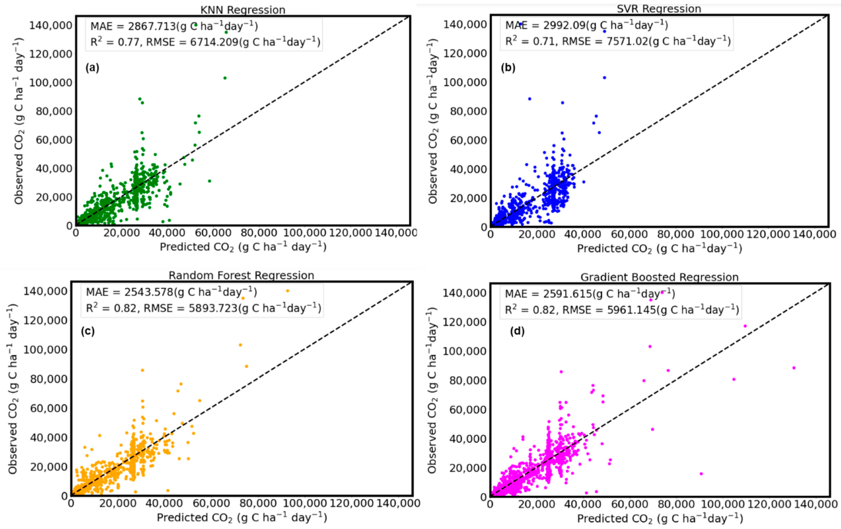
3.2. Model Performance Assessment

Model performance assessment aims to quantify the ability of the models developed to accurately generalize to new data that was not used to train the model. Three statistical criteria (R2, MAE, and RMSE) were used to assess how well the resulting models performed on the testing dataset not used in model development. Table 4 presents the evaluation metrics for the different predictive models.
The results from this modeling study indicate that the SVR model was the lowest performing model. The evaluation metrics of the SVR model on the training dataset were R2 = 0.74, MAE = 2923.69 g C ha−1 day−1, and RMSE = 6708.81 g C ha−1 day−1, whereas the evaluation metrics of the SVR model on the test dataset were R2 = 0.71, MAE = 2992.09 g C ha−1 day−1, and RMSE = 7571.02 g C ha−1 day−1. To achieve optimal performance when using the SVR algorithm on a test dataset, it is important to carefully choose the hyperparameters [62]. The training stage of the SVR algorithm found the optimal hyperparameters to achieve the best generalization of the model when predicting CO2 flux on the test dataset. Although the SVR algorithm has many hyperparameters, in this study, we chose four hyperparameters (C, ε, γ and the kernel function) that were tuned using the GridSearchCV module. According to Kaingo et al. [63], a successful SVR implementation depends on selecting a suitable kernel function, choice of the cost parameter C, and the “tube” insensitive variable ε. The “RBF” (radial basis function) performed better than the linear and sigmoid functions. Hamrani et al. [17] reported an R2 of 0.92 and 0.68 during training and testing when SVR was used to predict CO2 fluxes. Even though their model performed well on the training dataset, there was a high variability, which led to a lower performance on their test dataset. By comparison, the SVR model in our study was able to generalize fairly well to data that was not used to train the model, with an R2 value of 0.71.
A better performing algorithm was the KNN regression algorithm. The evaluation results on the training dataset using the KNN were: R2 = 0.80, MAE = 2679.03 g C ha−1 day−1, RMSE = 5910.76 g C ha−1 day−1 and the result for the test dataset were R2 = 0.77, MAE = 0.2867.71 g C ha−1 day−1, RMSE = 6714.21 g C ha−1 day−1. The hyperparameters tuned for the KNN were the K neighbors (in this case the number of measurements for soil CO2 fluxes) and the distance function used to estimate a new data point. The value for K was tuned and carefully chosen because a low value can lead to overfitting of the data, and a larger K value can lead to underfitting of the data [64]. The GridSearchCV module was used to test a range of K from 1 to 50 and the optimal K obtained was 8.
Tree-based regression algorithms are supervised machine learning algorithms that predict an output variable by building tree-like structures. The basic form of the tree-based algorithms is the decision tree algorithm. However, decision trees are prone to overfitting as the tree grows bigger and more complex [53]; thus, improved versions (RF and GB regression algorithms) of the decision tree algorithm were used in this study. In general, the tree-based regression algorithms (RF and GB) produced the most optimal models for simulating CO2 fluxes.
Among the four algorithms applied to simulate CO2 flux in this study, the RF and GB regression models were the best performing models when used to predict CO2 flux on an unseen test dataset, which is of more importance in estimating real world CO2 fluxes. On the training dataset, the evaluation metrics for the RF regression model were R2 = 0.87, MAE = 1968.07 g C ha−1 day−1, and RMSE = 4696.76 g C ha−1 day−1. On the test dataset, the evaluation metrics for RF were R2 = 0.82, MAE = 2543.58 g C ha−1 day−1, and RMSE = 5893.72 g C ha−1 day−1. The hyperparameters that were tuned to increase the performance of the RF regression model were the n_estimators, max_depth, max_features, and min_sample_leaf. Because the RF regression is a tree-based algorithm, n_estimators refers to the number of trees the algorithm built to estimate a mean prediction for a particular observation of CO2 flux. The optimum hyperparameters found using the GridSearchCV module for all the algorithms are shown in Table 5, and Figure 2 shows the performance metrics for predicted CO2 fluxes.
Hamrani et al. [17] reported an R2 of 0.96 and 0.75 during training and testing using an RF model to predict CO2 fluxes. Comparatively, the RF model developed in our study attained a higher predictive performance than that of Hamrani et al. [17] because our RF model achieved an R2 = 0.82. When using decision trees to develop models, each node of a tree is split using the best split among the predictors. However, an improved approach using the RF algorithm is to split each node using the best among a subset of predictors chosen at that node [65]. The combination of trees grown using random variables in the case of the RF algorithm increases accuracy because the variables are randomly chosen at each node [54]. Unlike simple regression models that depend on process-level understanding of flux variability, ML models such as RF utilize functional relationships between the predictors and the dependent variable that are learned during the training stage of the algorithm implementation [54].
The GB regression algorithm resulted in comparably high performance metrics on the training dataset when compared to the RF model. The performance metrics on the training dataset using GB regression were R2= 0.88, MAE = 2177.89g C ha−1 day−1, and RMSE = 4405.43g C ha−1 day−1. On the test dataset, it produced comparable model performance (i.e., R2 = 0.82, MAE = 2591.61g C ha−1 day−1, and RMSE = 5961.15g C ha−1 day−1) to that of the RF algorithm but higher than that of models produced by the SVR and KNN regression algorithms. To increase the accuracy of the models built using the GB regression algorithm, we used the GridSearchCV module in tuning the number of estimators (n_estimators), the learning rate, maximum depth (max_depth), the loss function, and alpha. The learning rate controls the contribution of each tree in the GB model and decreasing the learning rate increases the number of trees required [66]. The optimized hyperparameters chosen are shown in Table 3. Figure 3 shows a one-to-one scatter plot comparison of the four models we tested with their respective performance metrics.

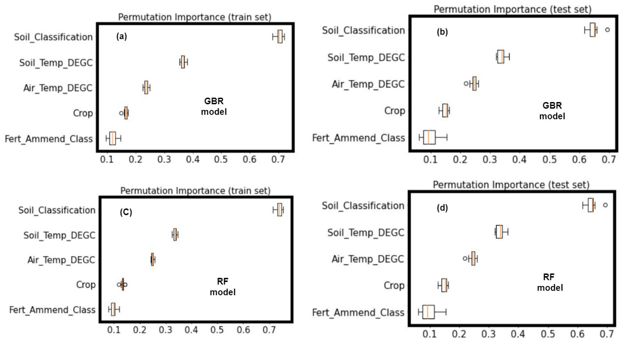
3.3. Important Model Predictors for Estimating Soil CO2 Fluxes

Model interpretation is key to understanding the practical implications of the drivers of soil CO2 fluxes in the GRACEnet database. Because ML models are not as interpretable as the process-based models, mechanistic models, or parametric models such as linear regression, it is not surprising that ML model interpretability is currently a “hot” topic of debate. In the ML research community, there is still no clear definition or evaluation criteria for interpretability [67]. In linear regression, one can easily interpret the model parameters (i.e., slope and intercept) and derive insights for practical interpretations. By contrast, ML methods have often been criticized for lacking interpretable parameters, especially neural networks, which have been described as a “black box” algorithm that is not easily understood [68]. Although traditional model estimation methods (e.g., linear regression) makes interpretation easier, complex non-linear models (e.g., GB and RF regression) are sometimes more accurate but do not necessarily yield intelligible parameters to infer mechanistic relationships [58].
Various methods have been developed that makes interpretation of the final models possible by simplifying the relationships between the predictors and the output variable. Interpretable here means the ability to extract relevant knowledge from the models developed with regards to relationships between variables [69]. Although several model independent methods (e.g., individual conditional expectation, covariate importance with permutation, partial dependence plots [70]) are currently available to interpret ML models, perhaps the most prominent and intuitive method is the permutation feature importance (PFI) proposed by Breiman [54]. PFI has been implemented as a function in Scikit-learn [38] and is used to determine the important predictors in models developed using the tree-based machine learning algorithms (RF and GB regression). First described by Breiman [54] for the random forest algorithm, PFI describes how important the various features/predictors are for predicting the performance of the models, regardless of the shape, i.e., linear or non-linear [71]. Thus, a predictor will be considered important if shuffling its value leads to an increase in the error rate of the prediction. In this study, we implemented PFI to help determine the influence of predictors in the final models.
Evaluation of the models developed in this study revealed the tree-based algorithms (RF regression and GB regression) to be the best performing models. Thus, PFI was performed on the RF and GB regression models using both the training dataset and the test dataset. The results of the PFI are shown in Figure 4. The GB regression and RF regression models both showed a similar ranking of predictors in the models. The soil classification within the site of measurement was ranked first for predicting soil CO2 fluxes. Although our hypothesis—that fertilizer amendment class was a useful predictor in ML models of CO2 fluxes—was supported, it was not the most important predictor. Soil classification, soil temperature, air temperature, and cropping system were found to be more important predictors of soil CO2 fluxes than the type of fertilizer amendment.
Soil temperature is a well-known predictor of the CO2 fluxes, and the results here are consistent with previous studies that show a link between soil temperature and soil GHG fluxes [3,17,28,72,73,74]. As the temperature of a soil increases, soil respiration increases, which leads to greater CO2 emissions and a positive feedback to CO2 fluxes associated with increased microbial metabolism [3]. The change in soil GHG emissions with an increase in soil temperature can be described with the temperature sensitivity factor, Q10 [3,75].
Soil moisture was not used as a predictor for any of the models as it showed a very weak correlation (0.08) with CO2 fluxes for the GRACEnet database. Although Abbasi [23] also found low correlation of soil moisture with CO2 emissions under a corn–soy rotation cropping system, they opted to include it in their model based on previous studies. Including soil moisture in the models studied here led to lower performance. Although short-term daily precipitation can influence soil CO2 fluxes [76], there was no relationship between daily precipitation and soil CO2 fluxes in the GRACEnet database; hence, it was not considered as a predictor for developing the models in this study.
Biogeochemical models and process-based models are guided by process level theory [21], but ML models can only be interpreted in the context of the data used to execute the prediction. The improvement in the accuracy when ML algorithms are used for modeling occurs because ML techniques use similarities between samples to estimate future samples, which is advantageous when the form of the relationship between the predictor and the output variable is unknown prior to analysis [77]. Although ML-based models are not inherently superior to process-based models, they can help complement process-based models by better identifying the key variables that are driving CO2 fluxes [21].
It should be noted that this study was primarily focused on comparing the predictive ability of various machine learning algorithms for simulating CO2 fluxes. Hence, the performance of the models developed in this study was not compared to models developed using the Denitrification Decomposition model (DNDC) or DAYCENT model, which have been used in previous studies to simulate CO2 fluxes. Secondly, even though the GRACEnet database contains data for N2O and CH4 soil fluxes, the five predictors chosen were not correlated to N2O and CH4 soil fluxes and so only CO2 fluxes were simulated. Despite these limitations, this study presents an alternative route to modeling CO2 fluxes that does not require extensive domain knowledge in soil biogeochemistry. Overall, the study demonstrates the suitability of tree-based machine learning algorithms in modeling CO2 emissions in cropping systems.

4. Conclusions

As more data are made publicly available from direct measurements, more synthesis tools will be needed to interpret the enormous amount of information in databases. With the availability of more data comes the need for methods to use these data to understand how soil properties influence the emission of GHGs. The advent of ML modeling algorithms within the past few decades has provided opportunities for the use of these available databases to analyze and simulate GHG fluxes in various cropping systems. In this study, we demonstrated the application of four popular ML algorithms (KNN regression, support vector regression, random forest regression, and gradient boosted regression) to simulate soil CO2 fluxes with available data from the GRACEnet database. Five predictors (air temperature, soil temperature, fertilizer amendment class, soil classification, crop) were selected to develop the models based on results from step-forward feature selection and correlation analysis. Among the four ML algorithms, the prediction based on the RF and GR regression models achieved the highest accuracy. Soil classification was the most important predictor variable evaluated in both the RF and GB models produced from ML methods.
Although the RF algorithm is robust when there are missing data in large datasets, RF should only be considered when there is no known linear relationship existing between predictors and output variables. If there is a linear relationship between predictors and output variables, it is appropriate to use linear regression instead. In addition, the validation dataset should be inspected to ensure that most of the data is not out of the range of the training dataset, as RF is inefficient in predicting values beyond the range of the training dataset. Although the GB algorithm usually attains the highest accuracy among most ML algorithms, there is always a trade-off between predictive power of GB and the computational power required to run the algorithm. More complexity in model hyperparameters results in greater computation time and expense for a user, especially when the number of “trees” exceeds 1000. Overall, the RF and GB algorithms are best suited for large datasets with non-linear relationships.
This study was primarily concerned with testing the capabilities of ML algorithms for simulating CO2 fluxes using minimal predictors (temperature, soil moisture, soil type, air temperature, cropping system, and the type of fertilization) in the GRACEnet database. Soil chemical properties (e.g., pH, CEC, organic carbon, and clay content) were not considered as predictors because there were many values missing in the GRACEnet database that could introduce bias and reduce model performance. Future studies can explore the suitability of applying other ML algorithms, e.g., artificial neural networks and XGBoost, to the GRACEnet database to determine if hyperparameter tuning can be improved and increase the performance of the algorithms in simulating GHG fluxes.

Author Contributions

Conceptualization, T.A.A. and S.C.D.; methodology, T.A.A. and S.C.D.; software, T.A.A.; validation, T.A.A. and S.C.D.; formal analysis, T.A.A. and S.C.D.; investigation, T.A.A. and S.C.D.; data curation, T.A.A.; writing—original draft preparation, T.A.A.; writing—review and editing, T.A.A. and S.C.D.; visualization, T.A.A.; funding acquisition, S.C.D. All authors have read and agreed to the published version of the manuscript.

Funding

This research received no external funding.

Data Availability Statement

The original data used in this study can be found at: https://data.nal.usda.gov/dataset/gracenet-greenhouse-gas-reduction-through-agricultural-carbon-enhancement-network (accessed on 8 February 2021). The redacted version can be obtained from the first author and is accessible from https://github.com/Toby4321/GRACEnet-Data (accessed on 23 October 2021).

Acknowledgments

The authors acknowledge work supported by the Agricultural Research Service under the ARS GRACEnet Project that made this study possible.

Conflicts of Interest

The authors declare no conflict of interest.

References

  1. Shabani, E.; Hayati, B.; Pishbahar, E.; Ghorbani, M.A.; Ghahremanzadeh, M. A novel approach to predict CO2 emission in the agriculture sector of Iran based on Inclusive Multiple Model. J. Clean. Prod. 2021, 279, 123708. [Google Scholar] [CrossRef]
  2. EPA U.S. Overview of Greenhouse Gases. Available online: https://www.epa.gov/ghgemissions/overview-greenhouse-gases (accessed on 30 May 2021).
  3. Oertel, C.; Matschullat, J.; Zurba, K.; Zimmermann, F.; Erasmi, S. Greenhouse gas emissions from soils—A review. Chem. Der Erde Geochem. 2016, 76, 327–352. [Google Scholar] [CrossRef] [Green Version]
  4. Zhang, K.; Zheng, H.; Chen, F.; Li, R.; Yang, M.; Ouyang, Z.; Lan, J.; Xiang, X. Impact of nitrogen fertilization on soil–Atmosphere greenhouse gas exchanges in eucalypt plantations with different soil characteristics in southern China. PLoS ONE 2017, 12, e0172142. [Google Scholar] [CrossRef] [PubMed] [Green Version]
  5. Post, W.M.; Emanuel, W.R.; Zinke, P.J.; Stangenberger, A.G. Soil carbon pools and world life zones. Nature 1982, 298, 156–159. [Google Scholar] [CrossRef]
  6. Yousaf, B.; Liu, G.; Wang, R.; Abbas, Q.; Imtiaz, M.; Liu, R. Investigating the biochar effects on C-mineralization and sequestration of carbon in soil compared with conventional amendments using the stable isotope (δ13C) approach. GCB Bioenergy 2017, 9, 1085–1099. [Google Scholar] [CrossRef]
  7. Paustian, K.; Lehmann, J.; Ogle, S.; Reay, D.; Robertson, G.P.; Smith, P. Climate-smart soils. Nature 2016, 532, 49–57. [Google Scholar] [CrossRef] [Green Version]
  8. Li, C. Quantifying greenhouse gas emissions from soils: Scientific basis and modeling approach. Soil Sci. Plant Nutr. 2007, 53, 344–352. [Google Scholar] [CrossRef] [Green Version]
  9. Liang, N.; Nakadai, T.; Hirano, T.; Qu, L.; Koike, T.; Fujinuma, Y.; Inoue, G. In situ comparison of four approaches to estimating soil CO2 efflux in a northern larch (Larix kaempferi Sarg.) forest. Agric. For. Meteorol. 2004, 123, 97–117. [Google Scholar] [CrossRef]
  10. Heinemeyer, A.; McNamara, N.P. Comparing the closed static versus the closed dynamic chamber flux methodology: Implications for soil respiration studies. Plant Soil 2011, 346, 145–151. [Google Scholar] [CrossRef]
  11. Gargiulo, O.; Morgan, K.T. Procedures to Simulate Missing Soil Parameters in the Florida Soils Characteristics Database. Soil Sci. Soc. Am. J. 2015, 79, 165–174. [Google Scholar] [CrossRef]
  12. Li, C.; Frolking, S.; Frolking, T.A. A model of nitrous oxide evolution from soil driven by rainfall events: 1. Model structure and sensitivity. J. Geophys. Res. Atmos. 1992, 97, 9759–9776. [Google Scholar] [CrossRef]
  13. Herbst, M.; Hellebrand, H.J.; Bauer, J.; Huisman, J.A.; Šimůnek, J.; Weihermüller, L.; Graf, A.; Vanderborght, J.; Vereecken, H. Multiyear heterotrophic soil respiration: Evaluation of a coupled CO2 transport and carbon turnover model. Ecol. Model. 2008, 214, 271–283. [Google Scholar] [CrossRef]
  14. Del Grosso, S.J.; Parton, W.J.; Adler, P.R.; Davis, S.C.; Keough, C.; Marx, E. DayCent model simulations for estimating soil carbon dynamics and greenhouse gas fluxes from agricultural production systems. In Managing Agricultural Greenhouse Gases; Liebig, M.A., Franzluebbers, A.J., Follett, R.F., Eds.; Elsevier: Amsterdam, The Netherlands, 2012; pp. 341–353. [Google Scholar]
  15. Del Grosso, S.J.; Ojima, D.S.; Parton, W.J.; Stehfest, E.; Heistemann, M.; Deangelo, B.; Rose, S. Global scale DAYCENT model analysis of greenhouse gas emissions and mitigation strategies for cropped soils. Glob. Planet. Change 2009, 67, 44–50. [Google Scholar] [CrossRef]
  16. Ahuja, L.; Rojas, K.; Hanson, J.D. Root Zone Water Quality Model: Modelling Management Effects on Water Quality and Crop Production; Water Resources Publication: Littleton, CO, USA, 2000.
  17. Hamrani, A.; Akbarzadeh, A.; Madramootoo, C.A. Machine learning for predicting greenhouse gas emissions from agricultural soils. Sci. Total Environ. 2020, 741, 140338. [Google Scholar] [CrossRef] [PubMed]
  18. Liakos, K.G.; Busato, P.; Moshou, D.; Pearson, S.; Bochtis, D. Machine learning in agriculture: A review. Sensors 2018, 18, 2674. [Google Scholar] [CrossRef] [PubMed] [Green Version]
  19. Twarakavi, N.K.C.; Šimůnek, J.; Schaap, M.G. Development of Pedotransfer Functions for Estimation of Soil Hydraulic Parameters using Support Vector Machines. Soil Sci. Soc. Am. J. 2009, 73, 1443–1452. [Google Scholar] [CrossRef] [Green Version]
  20. Baker, R.E.; Peña, J.-M.; Jayamohan, J.; Jérusalem, A. Mechanistic models versus machine learning, a fight worth fighting for the biological community? Biol. Lett. 2018, 14, 20170660. [Google Scholar] [CrossRef]
  21. Saha, D.; Basso, B.; Robertson, G.P. Machine learning improves predictions of agricultural nitrous oxide (N2O) emissions from intensively managed cropping systems. Environ. Res. Lett. 2021, 16, 024004. [Google Scholar] [CrossRef]
  22. Ebrahimi, M.; Sarikhani, M.R.; Safari Sinegani, A.A.; Ahmadi, A.; Keesstra, S. Estimating the soil respiration under different land uses using artificial neural network and linear regression models. CATENA 2019, 174, 371–382. [Google Scholar] [CrossRef]
  23. Abbasi, N.A.; Hamrani, A.; Madramootoo, C.A.; Zhang, T.; Tan, C.S.; Goyal, M.K. Modelling carbon dioxide emissions under a maize-soy rotation using machine learning. Biosyst. Eng. 2021, 212, 1–18. [Google Scholar] [CrossRef]
  24. Freitas, L.P.; Lopes, M.L.; Carvalho, L.B.; Panosso, A.R.; Júnior, N.L.S.; Freitas, R.L.; Minussi, C.R.; Lotufo, A.D. Forecasting the spatiotemporal variability of soil CO2 emissions in sugarcane areas in southeastern Brazil using artificial neural networks. Environ. Monit. Assess. 2018, 190, 741. [Google Scholar] [CrossRef]
  25. Philibert, A.; Loyce, C.; Makowski, D. Prediction of N2O emission from local information with Random Forest. Environ. Pollut. 2013, 177, 156–163. [Google Scholar] [CrossRef]
  26. Tavares, R.L.M.; Oliveira, S.R.D.M.; Barros, F.M.M.D.; Farhate, C.V.V.; Souza, Z.M.D.; Scala Junior, N.L. Prediction of soil CO2 flux in sugarcane management systems using the Random Forest approach. Sci. Agric. 2018, 75, 281–287. [Google Scholar] [CrossRef] [Green Version]
  27. Gauder, M.; Butterbach-Bahl, K.; Graeff-Hönninger, S.; Claupein, W.; Wiegel, R. Soil-derived trace gas fluxes from different energy crops - results from a field experiment in Southwest Germany. GCB Bioenergy 2012, 4, 289–301. [Google Scholar] [CrossRef]
  28. Adjuik, T.; Rodjom, A.M.; Miller, K.E.; Reza, M.T.M.; Davis, S.C. Application of Hydrochar, Digestate, and Synthetic Fertilizer to a Miscanthus x giganteus Crop: Implications for Biomass and Greenhouse Gas Emissions. Appl. Sci. 2020, 10, 8953. [Google Scholar] [CrossRef]
  29. Snyder, C.S.; Bruulsema, T.W.; Jensen, T.L.; Fixen, P.E. Review of greenhouse gas emissions from crop production systems and fertilizer management effects. Agric. Ecosyst. Environ. 2009, 133, 247–266. [Google Scholar] [CrossRef]
  30. Davis, S.C.; Parton, W.J.; Dohleman, F.G.; Smith, C.M.; Grosso, S.D.; Kent, A.D.; DeLucia, E.H. Comparative Biogeochemical Cycles of Bioenergy Crops Reveal Nitrogen-Fixation and Low Greenhouse Gas Emissions in a Miscanthus × giganteus Agro-Ecosystem. Ecosystems 2009, 13, 144–156. [Google Scholar] [CrossRef]
  31. Don, A.; Osborne, B.; Hastings, A.; Skiba, U.; Carter, M.S.; Drewer, J.; Flessa, H.; Freibauer, A.; Hyvönen, N.; Jones, M.B.; et al. Land-use change to bioenergy production in Europe: Implications for the greenhouse gas balance and soil carbon. GCB Bioenergy 2012, 4, 372–391. [Google Scholar] [CrossRef] [Green Version]
  32. Jawson, M.; Shafer, S.; Franzluebbers, A.; Parkin, T.; Follett, R. GRACEnet: Greenhouse gas reduction through agricultural carbon enhancement network. Soil Tillage Res. 2005, 83, 167–172. [Google Scholar] [CrossRef]
  33. Del Grosso, S.J.; White, J.W.; Wilson, G.; Vandenberg, B.; Karlen, D.L.; Follett, R.F.; Johnson, J.M.F.; Franzluebbers, A.J.; Archer, D.W.; Gollany, H.T.; et al. Introducing the GRACEnet/REAP Data Contribution, Discovery, and Retrieval System. J. Environ. Qual. 2013, 42, 1274–1280. [Google Scholar] [CrossRef] [PubMed] [Green Version]
  34. Kotsiantis, S.B.; Kanellopoulos, D.; Pintelas, P.E. Data preprocessing for supervised leaning. Int. J. Comput. Sci. 2006, 1, 111–117. [Google Scholar]
  35. Lakshminarayan, K.; Harp, S.A.; Samad, T. Imputation of missing data in industrial databases. Appl. Intell. 1999, 11, 259–275. [Google Scholar] [CrossRef]
  36. Derksen, S.; Keselman, H.J. Backward, forward and stepwise automated subset selection algorithms: Frequency of obtaining authentic and noise variables. Br. J. Math. Stat. Psychol. 1992, 45, 265–282. [Google Scholar] [CrossRef]
  37. Guyon, I.; Elisseeff, A. An introduction to variable and feature selection. J. Mach. Learn. Res. 2003, 3, 1157–1182. [Google Scholar]
  38. Pedregosa, F.; Varoquaux, G.; Gramfort, A.; Michel, V.; Thirion, B.; Grisel, O.; Blondel, M.; Prettenhofer, P.; Weiss, R.; Dubourg, V. Scikit-learn: Machine learning in Python. J. Mach. Learn. Res. 2011, 12, 2825–2830. [Google Scholar]
  39. Hastie, T.; Tibshirani, R.; Friedman, J. The Elements of Statistical Learning: Data Mining, Inference, and Prediction; Springer Science & Business Media: Berlin/Heidelberg, Germany, 2009. [Google Scholar]
  40. Witten, I.H.; Frank, E. Data Mining: Practical Machine Learning Tools and Techniques with Java Implementations; Acm Sigmod Record: Cambridge, MA, USA, 2002; Volume 31, pp. 76–77. [Google Scholar]
  41. Yang, L.; Shami, A. On hyperparameter optimization of machine learning algorithms: Theory and practice. Neurocomputing 2020, 415, 295–316. [Google Scholar] [CrossRef]
  42. McKinney, W. Python for Data Analysis: Data Wrangling with Pandas, NumPy, and IPython; O’Reilly Media, Inc.: Newton, MA, USA, 2012. [Google Scholar]
  43. Kluyver, T.; Ragan-Kelley, B.; Pérez, F.; Granger, B.E.; Bussonnier, M.; Frederic, J.; Kelley, K.; Hamrick, J.B.; Grout, J.; Corlay, S. Jupyter Notebooks-a Publishing Format for Reproducible Computational Workflows; IOS Press: Amsterdam, The Netherlands, 2016; Volume 2016. [Google Scholar]
  44. Raschka, S. MLxtend: Providing machine learning and data science utilities and extensions to Python’s scientific computing stack. J. Open Source Softw. 2018, 3, 638. [Google Scholar] [CrossRef]
  45. Ayodele, T.O. Types of machine learning algorithms. New Adv. Mach. Learn. 2010, 3, 19–48. [Google Scholar]
  46. Kotsiantis, S.B.; Zaharakis, I.; Pintelas, P. Supervised machine learning: A review of classification techniques. In Real Word AI Systems with Applications in eHealth, Hci, Information Retrieval and Pervasive Technologies; IOS Press: Amsterdam, The Netherlands; Washington, DC, USA, 2007; Volume 160, pp. 3–24. [Google Scholar]
  47. Achieng, K.O. Modelling of soil moisture retention curve using machine learning techniques: Artificial and deep neural networks vs support vector regression models. Comput. Geosci. 2019, 133, 104320. [Google Scholar] [CrossRef]
  48. Awad, M.; Khanna, R. Support Vector Regression. In Efficient Learning Machines; Apress: Berkeley, CA, USA, 2015; pp. 67–80. [Google Scholar]
  49. Üstün, B.; Melssen, W.J.; Buydens, L.M. Facilitating the application of support vector regression by using a universal Pearson VII function based kernel. Chemom. Intell. Lab. Syst. 2006, 81, 29–40. [Google Scholar] [CrossRef]
  50. Müller, A.C.; Guido, S. Introduction to Machine Learning with Python: A Guide for Data Scientists; O’Reilly Media, Inc.: Sebastopol, CA, USA, 2016. [Google Scholar]
  51. Imandoust, S.B.; Bolandraftar, M. Application of k-nearest neighbor (knn) approach for predicting economic events: Theoretical background. Int. J. Eng. Res. Appl. 2013, 3, 605–610. [Google Scholar]
  52. Ray, S. A Quick Review of Machine Learning Algorithms. In Proceedings of the International Conference on Machine Learning, Big Data, Cloud and Parallel Computing (Com-IT-Con), Faridabad, India, 14–16 February 2019; p. 5. [Google Scholar]
  53. Ho, T.K. Random decision forests. In Proceedings of the 3rd International Conference on Document Analysis and Recognition, Montreal, QC, Canada, 14–16 August 1995; pp. 278–282. [Google Scholar]
  54. Breiman, L. Random forests. Mach. Learn. 2001, 45, 5–32. [Google Scholar] [CrossRef] [Green Version]
  55. Horning, N. Random Forests: An algorithm for image classification and generation of continuous fields data sets. In Proceedings of the International Conference on Geoinformatics for Spatial Infrastructure Development in Earth and Allied Sciences, Osaka, Japan, 9–11 December 2010. [Google Scholar]
  56. Zhang, H.; Nettleton, D.; Zhu, Z. Regression-enhanced random forests. arXiv 2019, arXiv:1904.10416. [Google Scholar]
  57. Friedman, J.H. Stochastic gradient boosting. Comput. Stat. Data Anal. 2002, 38, 367–378. [Google Scholar] [CrossRef]
  58. Molnar, C.; König, G.; Herbinger, J.; Freiesleben, T.; Dandl, S.; Scholbeck, C.A.; Casalicchio, G.; Grosse-Wentrup, M.; Bischl, B. Pitfalls to avoid when interpreting machine learning models. arXiv 2020, arXiv:2007.04131. [Google Scholar]
  59. Sandri, M.; Zuccolotto, P. Variable Selection Using Random Forests. In Data Analysis, Classification and the Forward Search; Springer: Berlin/Heidelberg, Germany, 2006; pp. 263–270. [Google Scholar]
  60. O’Brien, R.M. A Caution Regarding Rules of Thumb for Variance Inflation Factors. Qual. Quant. 2007, 41, 673–690. [Google Scholar] [CrossRef]
  61. Chandra, B. Gene Selection Methods for Microarray Data. In Applied Computing in Medicine and Health; Elsevier: Amsterdam, The Netherlands, 2016; pp. 45–78. [Google Scholar]
  62. Elbisy, M.S. Support vector machine and regression analysis to predict the field hydraulic conductivity of sandy soil. KSCE J. Civ. Eng. 2015, 19, 2307–2316. [Google Scholar] [CrossRef]
  63. Kaingo, J.; Tumbo, S.D.; Kihupi, N.I.; Mbilinyi, B.P. Prediction of Soil Moisture-Holding Capacity with Support Vector Machines in Dry Subhumid Tropics. Appl. Environ. Soil Sci. 2018, 2018, 9263296. [Google Scholar] [CrossRef] [Green Version]
  64. Altman, N.S. An Introduction to Kernel and Nearest-Neighbor Nonparametric Regression. Am. Stat. 1992, 46, 175–185. [Google Scholar] [CrossRef] [Green Version]
  65. Liaw, A.; Wiener, M. Classification and regression by randomForest. R News 2002, 2, 18–22. [Google Scholar]
  66. Elith, J.; Leathwick, J.R.; Hastie, T. A working guide to boosted regression trees. J. Anim. Ecol. 2008, 77, 802–813. [Google Scholar] [CrossRef] [PubMed]
  67. Gilpin, L.H.; Bau, D.; Yuan, B.Z.; Bajwa, A.; Specter, M.; Kagal, L. Explaining explanations: An overview of interpretability of machine learning. In Proceedings of the 2018 IEEE 5th International Conference on Data Science and Advanced Analytics (DSAA), Turin, Italy, 1–3 October 2018; pp. 80–89. [Google Scholar]
  68. Lipton, Z.C. The Mythos of Model Interpretability: In machine learning, the concept of interpretability is both important and slippery. Queue 2018, 16, 31–57. [Google Scholar] [CrossRef]
  69. Murdoch, W.J.; Singh, C.; Kumbier, K.; Abbasi-Asl, R.; Yu, B. Interpretable machine learning: Definitions, methods, and applications. arXiv 2019, arXiv:1901.04592. [Google Scholar] [CrossRef] [PubMed] [Green Version]
  70. Wadoux, A.M.-C.; Molnar, C. Beyond prediction: Methods for interpreting complex models of soil variation. Geoderma 2021. [Google Scholar] [CrossRef]
  71. Casalicchio, G.; Molnar, C.; Bischl, B. Visualizing the feature importance for black box models. In Proceedings of the Joint European Conference on Machine Learning and Knowledge Discovery in Databases, Dublin, Ireland, 10–14 September 2018; pp. 655–670. [Google Scholar]
  72. Wachiye, S.; Merbold, L.; Vesala, T.; Rinne, J.; Räsänen, M.; Leitner, S.; Pellikka, P. Soil greenhouse gas emissions under different land-use types in savanna ecosystems of Kenya. Biogeosciences 2020, 17, 2149–2167. [Google Scholar] [CrossRef] [Green Version]
  73. Schaufler, G.; Kitzler, B.; Schindlbacher, A.; Skiba, U.; Sutton, M.A.; Zechmeister-Boltenstern, S. Greenhouse gas emissions from European soils under different land use: Effects of soil moisture and temperature. Eur. J. Soil Sci. 2010, 61, 683–696. [Google Scholar] [CrossRef]
  74. Schindlbacher, A.; Zechmeister-Boltenstern, S.; Butterbach-Bahl, K. Effects of soil moisture and temperature on NO, NO2, and N2O emissions from European forest soils. J. Geophys. Res. Atmos. 2004, 109, D17. [Google Scholar] [CrossRef]
  75. Lloyd, J.; Taylor, J.A. On the Temperature Dependence of Soil Respiration. Funct. Ecol. 1994, 8, 315. [Google Scholar] [CrossRef]
  76. Ni, X.; Liao, S.; Wu, F.; Groffman, P.M. Short-term precipitation pulses stimulate soil CO2 emission but do not alter CH4 and N2O fluxes in a northern hardwood forest. Soil Biol. Biochem. 2019, 130, 8–11. [Google Scholar] [CrossRef]
  77. Nemes, A.; Rawls, W.J.; Pachepsky, Y.A. Use of the nonparametric nearest neighbor approach to estimate soil hydraulic properties. Soil Sci. Soc. Am. J. 2006, 70, 327–336. [Google Scholar] [CrossRef]
Figure 1. Summary of steps for developing models to predict CO2 flux using machine learning algorithms.
Agronomy 12 00197 g001
Figure 2. Pearson heat map showing a correlation matrix between the predictor variables and CO2 flux.
Agronomy 12 00197 g002
Figure 3. Scatter plots of observed and model predicted CO2 (n = 1573) on the test datasets. KNN regression (a), SVR regression (b), random forest regression (c), and gradient boosted regression (d). The dotted diagonal line represents the 1:1 mapping of the observed vs predicted.
Agronomy 12 00197 g003
Figure 4. Permutation feature importance (PFI) of the five predictors: (a) shows the PFI on the training dataset of the GB regression model; (b) shows the PFI on the test dataset of the GB regression model; (c) shows the PFI on the training dataset of the RF model; and (d) shows the permutation importance on the test dataset of the RF model. Soil_Classification, soil classification; Soil_temp_DEGC, soil temperature (°C); Air_Temp_DEGC, air temperature (°C); Crop, cropping system; Fert_Ammend_Class, type of fertilizer amended to the crops.
Agronomy 12 00197 g004
Table 1. Summary of relevant studies that used machine learning (ML) to simulate soil GHGs.
StudyML Method UsedKey Highlight
Hamrani et al. [17]FNN, RBFNN, ExNN, LSTM, DBN, CNN, LASSO, RFR, and SVRLSTM model predicted the highest accuracy metrics on CO2 fluxes with (R2 = 0.87 and RMSE = 30.3 mg·m−2·h−1).
Saha et al. [21]RFRF model explained 51% of variation in daily N2O fluxes upon coupling with a cropping systems model used to predict daily soil nitrogen availability.
Ebrahimi et al. [22]ANN, LRANN model could predict basal respiration with R2 = 0.66 and substrate induced respiration with R2 = 0.52 respectively.
Abbasi et al. [23]SVM, RF, LASSO, FNN, RBFNN, and ELMRF attained optimal performance on predicting CO2 emissions with R2 = 0.86 and RMSE = 3.05 Kg ha−1 d−1.
Freitas et al. [24]ANNThe ANN model predicted CO2 fluxes with R2 = 0.80; mean absolute percentage error (MAPE) = 12.0591.
Philibert et al. [25]RFRF model predicted soil N2O fluxes with Root mean square error of prediction (RMSE) of 2.99 kg N ha−1 year−1).
Tavares et al. [26]RFRF model predicted soil CO2 fluxes with R2 = 0.80.
Abbreviations: FNN, Feed-forward neural networks; RBFNN, Radial basis function neural network; ExNN, Extreme neural network; LSTM, Long short-term memory network; DBN, Deep belief network; CNN, Convolutional neural network; LASSO, Least Absolute Shrinkage and Selection Operator; RF, Random Forest Regression; SVR, Support Vector Regression; ANN, Artificial neural networks; Linear regression (LR); ELM, Extreme learning machine.
Table 2. Summary of machine learning techniques used for predicting CO2 fluxes in this study.
TechniqueOperating PrincipleProsCons
Support vector regression (SVR)SVR works by regressing a dependent variable on an independent variable according to a weight vector and a bias term. Regression functions are learned by mapping data onto a high-dimensional feature space known as kernelling [47,48]Excellent generalization capability, with high prediction accuracy.
Performs well for data with high dimensions [48].
Choosing appropriate hyperparameters, especially kernel functions, is a difficult task [49].
Inefficient when dealing with large datasets.
K-Nearest Neighbor regression (KNN) The KNN regression model is an adaptation of the KNN classification algorithm whereby predictions for new instances are made based on the average of the values of its “K” nearest (most similar) neighbors in the training dataset [50].Relatively easy to implement because you only need to specify two parameters i.e., K and the distance function.
Robust to noisy training data and works effectively with large training data [51].
Computationally expensive when data is large because the algorithm computes distances of each query instance to all training samples [51].
Sensitive to missing data and outliers which can lead to reduction in accuracy [52].
Random forest regression (RF)RF is an ensemble algorithm based on the decision tree algorithm whereby several decision trees are constructed during training of the data and outputting the mean prediction of the individual trees [53]. The dataset is split into several segments by posing a series of questions about the features of the dataset (predictors) and a final decision of the class of a new prediction is made based on the outcome of the individual trees [54].Reduces overfitting and variance unlike in decision trees since it creates several trees using a subset of the data to predict an output.
Robust to missing values and outliers in a dataset [54].
Tends to overestimate low values and underestimate high values because the output value of a prediction is the average of several decision trees [55].
Inefficient at extrapolating during prediction beyond the the range of the training dataset [56].
Gradient boosted regression (GB)GB uses the technique of boosting to combine many relatively simple regression tree models, predicting their pseudo residuals, and fitting new models based on the pseudo residuals. New regression trees are built based on the same predictors used to predict the residuals for all samples in the training dataset until further addition of trees does not significantly reduce the residuals [57].Prediction accuracy usually higher than other regression models.
Has several hyperparameters that can be tuned to increase performance of models.
While it gives higher accuracy, GB does not necessarily yield intelligible parameters making interpretation of the model difficult [58].
Can be computationally expensive since it requires a large number of trees for optimal performance.
Table 3. Forward feature selection on the training dataset.
Best Predictor CombinationNumber of
Predictors Chosen
R2
Soil classification10.63
Air temperature, soil classification20.74
Air temperature, soil classification, fertilization amendment class30.76
Air temperature, soil classification, crop, and fertilization amendment class40.77
Air temperature, soil temperature, soil classification, fertilization amendment class, crop50.76
Air temperature, soil temperature, soil moisture, soil classification, fertilization amendment class, crop60.76
Table 4. Evaluation metrics of machine learning models for predicting CO2 fluxes in bioenergy crops.
Training DatasetTesting Dataset
ModelR2RMSE
(g C ha−1
day−1)
MAE
(g C ha−1 day−1)
R2RMSE
(g C ha−1 day−1)
MAE
(g C ha−1 day−1)
Support Vector Regression0.746708.812923.690.717571.022992.09
KNN Regression0.805910.762679.030.776714.212867.71
Random Forest0.874696.761968.070.825893.722543.58
Gradient Boosted Regression0.884405.432177.890.825961.152591.61
Table 5. Optimum hyperparameters used for predicting CO2 fluxes.
Learning AlgorithmHyperparameter
K Nearest Neighbor Regression (KNN)n_neighbors = 8, metric = “manhattan”
Support Vector Regression (SVR)kernel = ‘rbf’, C = 4000, ε = 0.001, and γ = 1.2
Gradient Boosted Regression (GB)n_estimators = 50, learning rate = 0.1, max_depth = 10, loss = ‘huber’, alpha = 0.99
Random Forest Regression (RF)n_estimators = 80, max_depth = 30, max_features = ‘sqrt’ min_sample_leaf = 2
Publisher’s Note: MDPI stays neutral with regard to jurisdictional claims in published maps and institutional affiliations.

