Validation of Rapid and Low-Cost Approach for the Delineation of Zone Management Based on Machine Learning Algorithms

Abstract

Proximal soil sensors are receiving strong attention from several disciplinary fields, and this has led to a rise in their availability in the market in the last two decades. The aim of this work was to validate agronomically a zone management delineation procedure from electromagnetic induction (EMI) maps applied to two different rainfed durum wheat fields. The k-means algorithm was applied based on the gap statistic index for the identification of the optimal number of management zones and their positions. Traditional statistical analysis was performed to detect significant differences in soil characteristics and crop response of each management zones. The procedure showed the presence of two management zones at both two sites under analysis, and it was agronomically validated by the significant difference in soil texture (+24.17%), bulk density (+6.46%), organic matter (+39.29%), organic carbon (+39.4%), total carbonates (+25.34%), total nitrogen (+30.14%), protein (+1.50%) and yield data (+1.07 t ha⁻¹). Moreover, six unmanned aerial vehicle (UAV) flight missions were performed to investigate the relationship between five vegetation indexes and the EMI maps. The results suggest performing the multispectral images acquisition during the flowering phenological stages to attribute the crop spatial variability to different soil proprieties.

1. Introduction

The current social context requires an increase in food production, improvement of its quality characteristics and greater environmental sustainability in the management of agricultural systems. Technological innovation plays a great role in making agriculture more efficient and sustainable.

On the 1 June 2018, the European Commission set goals for the new Common Agricultural Policy (CAP) for beyond 2020, focusing on the contribution of innovation and sustainability of crop production in Italy (through Regional Agricultural Policies), as for the rest of Europe (EIP-AGRI partnership). One of the key points reported is the necessity of effective nutrient management, more specifically, avoiding environmental losses and preserving yields [1].

Uniform management of fields does not consider spatial variability, and it is not the most effective management strategy. Precision agriculture is considered the most viable approach for achieving sustainable agriculture [2]. Soil is the temporal result of several factors such as the atmosphere, biosphere, lithosphere and hydrosphere [3]. Such variability may act over different spatial and temporal scales and affects crop yield both quantitatively and qualitatively [4].

The use of precision farming techniques (PA) is proposed as a solution, which would combine proximal and remote sensors [5] to follow and measure the spatial-temporal variability of the soil and crop during all growing seasons. Therefore, the soil plays a crucial role in the identification of zones within the field [6].

Among the different geophysical properties to better understand spatial variability of the soil, apparent electrical conductivity of the soil (ECa) is widely used by scientists [2,7,8] and is generally measured by electromagnetic induction (EMI) sensors. EMI has the advantages over traditional methods to collect soil information quickly, easily, at a relatively low cost and with a large volume of data collected [9].

The correct definition of management zones constitutes an important task to manage spatial variability within the field properly [10]. There are different techniques to delineate management zones taking into account soil or vegetation properties separately [11,12,13] or in combination, through classification techniques [10,13,14,15,16] or informed clustering based on functional relations [17,18], to account for response space-time dependence with spatially dense data, data misalignment in both space and time and repeated covariate measurements [18].

However, cluster analysis algorithms [19,20] are the basis of a direct approach to dividing a field using different layers of information stored in a geographical information system (GIS). Taking into account that data used to define management zones are usually related [15], it is possible to summarize the information by means of principal component analysis. Finally, the values of the main principal components can be interpolated and mapped, and these surfaces can be used to generate management zones by cluster analysis [11,12].

Irrespective of the approach used, defining an algorithm that will effectively partition a field in homogeneous zones remains one of the main challenges for precision agriculture [21]. Creating an algorithm requires the discretization and clustering of one or more continuous mapped variables that may influence yield in various, possibly non-linear ways. Several approaches were proposed in the literature, such as k-clustering, multivariate geostatistical methods [22,23], and GIS layering [24]. These approaches are powerful in their capacity to cluster high-dimensional datasets (i.e., including multiple variables), but they may not be easy to use because they do not offer a direct association of the classes to productivity or variability.

The cost-effectiveness of precision agriculture depends upon the cost of defining zones within fields, the temporal stability of these zones and the differences in responsiveness (yield and quality) of the zones submitted to differential treatment.

Delineation of management zones can be based on spatial variation in either crop yield or factors affecting the yield locally [23,25].

PA requires high-resolution spatial and temporal information, but traditional soil sampling and laboratory analyses are expensive, labor-intensive and require many samples [5].

By means of continuous soil and crop monitoring activity, the site-specific-nitrogen-management (SSNM) can be applied [23]. The SSNM is based on the delineation of homogeneous zones within the field, between which different doses of fertilizer should be applied [9].

Particularly, SSNM is a form of precision agriculture whereby decisions on resource application and agronomic practices are improved to match soil and crop requirements better. The SSNM allows the division of a field into areas that have internally the same characteristics but differ from each other [19].

In order to produce the homogeneous zone map, we need to monitor the field over time by using several sensors. Depending on the type of sensor used and analysis performed, several authors provided different approaches to define the homogeneous zones.

The authors of [26] proposed a multi-source geostatistical approach, [27] evaluated 20 different unsupervised machine learning algorithms, while [28] used the Self-Organizing Maps.

The aim of our contribution is to validate the k-means algorithm to delineate homogeneous management zones. The k-means algorithm uses low-cost resistivity maps created by an electromagnetic induction method as a source of data. The proposed approach could be used to easily reconduct the spatial variability of the soil in homogeneous management zones statistically different from each other for high-quality prescriptions maps for the precision farming application.

2. Materials and Methods

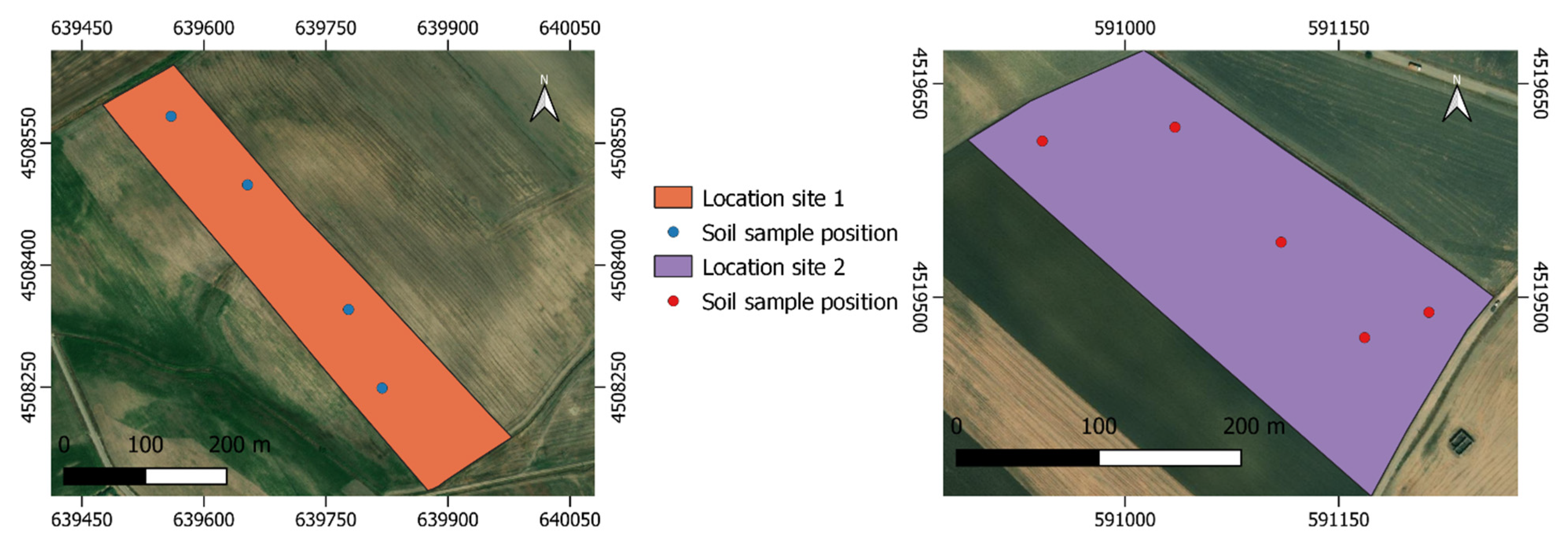
2.1. Experimental Sites Description

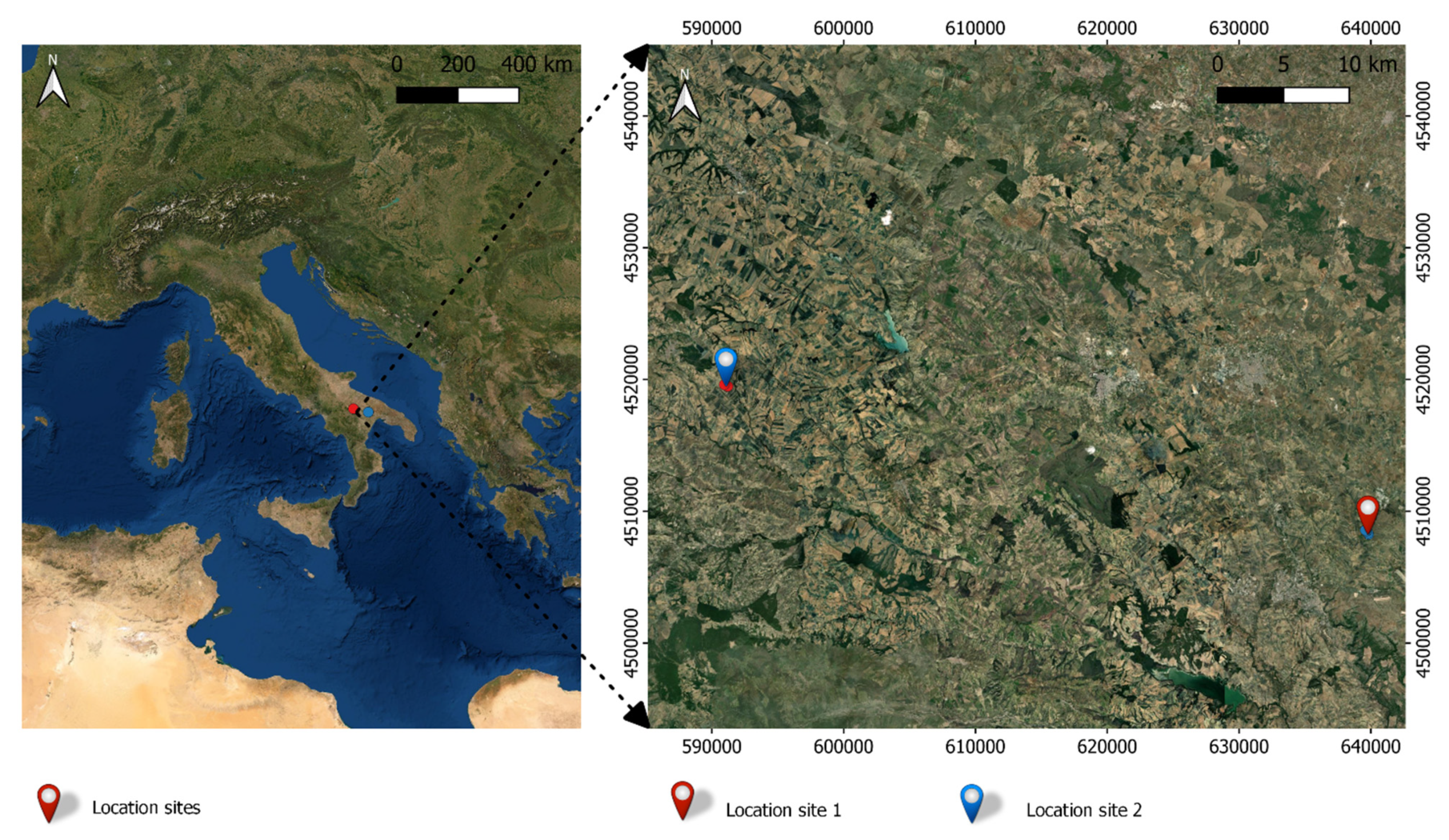
The method was tested on two experimental sites (Figure 1). In both sites, three different homogeneous zones (ZH) were identified by resistivity maps created by an electromagnetic induction (EMI), which were subsequently identified with the letters a, b, c. In these three areas, two different fertilization applications were tested: variable rate (VRT) and uniform (UA).

In 2019–2020 at site 1 Az. Agricola F.lli Lillo (Matera) latitude: 40.712640° longitude 16.656343° (Figure 2) on a study area of 6.65 ha, the experiment was conducted with durum wheat (Triticum durum L., var PR22D89) with sod seeding (7 January 2020).

In 2018–2019 at site 2 Genzano di Lucania (PZ) latitude: 40.82° N, longitude: 16.08° N (Figure 2), the study area (4.93 ha) was located on the clayey hills of the Bradanica grave and the basin of Sant’Arcangelo. The experiment was conducted with durum wheat (Triticum durum L., var Tirex). The inter-row spacing of 0.13 m and 250 kg ha⁻¹ of seeds was used. Soil tillage consisted of a 40 cm deep plowing (28 August 2018) and two harrowing (11 November 2018 and 5 December 2018) (Figure 2).

The crop potential N uptake was estimated by the nitrogen content in the yield in each homogeneous area and was corrected considering the nitrogen provided by mineralization of the organic matter by using the agri-environmental measures adopted within the Rural Development Plans at a local scale (https://www.regione.marche.it/Regione-Utile/Agricoltura-Sviluppo-Rurale-e-Pesca/Produzione-Integrata#Tecniche-Agronomiche, 15 December 2021). N mineralization was calculated considering the content of organic matter in the soil profile explored by the roots, its content in organic N and by the mineralization efficiency which in turn depends on the carbon/nitrogen ratio of the soil (1 for C/N < 9; 0.5 for C/N > 9, 0 for C/N < 12) (https://www.regione.marche.it/Regione-Utile/Agricoltura-Sviluppo-Rurale-e-Pesca/Produzione-Integrata#Tecniche-Agronomiche, 15 December 2021).

For the VRT treatment, the N doses applied in each area through a variable rate spreader are reported in

Table 1. Nitrogen management of site 1.

Distribution Mode	Dose of Nitrogen (kg ha−1 N)
Uniform rate of application (UA) area a, b, c	150 kg ha−1 of N
Variable Rate (VRT)	Zone a: 78 kg ha−1 N + 40 kg ha−1 N (pre-sowing) = 118 kg ha−1 N tot. Zone b: 93 kg ha−1 N + 40 kg ha−1 N (pre-sowing) = 133 kg ha−1 N tot. Zone c: 99 kg ha−1 N + 40 kg ha−1 N (pre-sowing) = 139 kg ha−1 N tot.

for site 1 and

Table 2. Nitrogen management of site 2.

Distribution Mode	Dose of N (kg ha−1 N)
Uniform rate of application (UA) area a, b, c	120 kg ha−1 of N
Variable Rate (VRT)	Zone a: 121.44 kg ha−1 N + 35 kg ha−1 N (pre-sowing) = 156.4 kg ha−1 N tot. Zone b: 63.44 kg ha−1 N + 35 kg ha−1 N (pre-sowing) = 98.3 kg ha kg ha−1 N tot. Zone c: 35.9 kg ha−1 N + 35 kg ha−1 N (pre-sowing) = 70.9 kg ha−1 N tot.

for site 2. For each treatment, plots of 2 m × 2 m replicated three times inside each of the homogeneous areas identified in the field were established. In all such plots, a dose of N uniform was applied, which corresponds to the amount generally applied by the farmer and slightly over the average of the dose of N applied in the three zones. The fertilizer was manually spread in UA.

2.2. Soil and Crop Samples Position

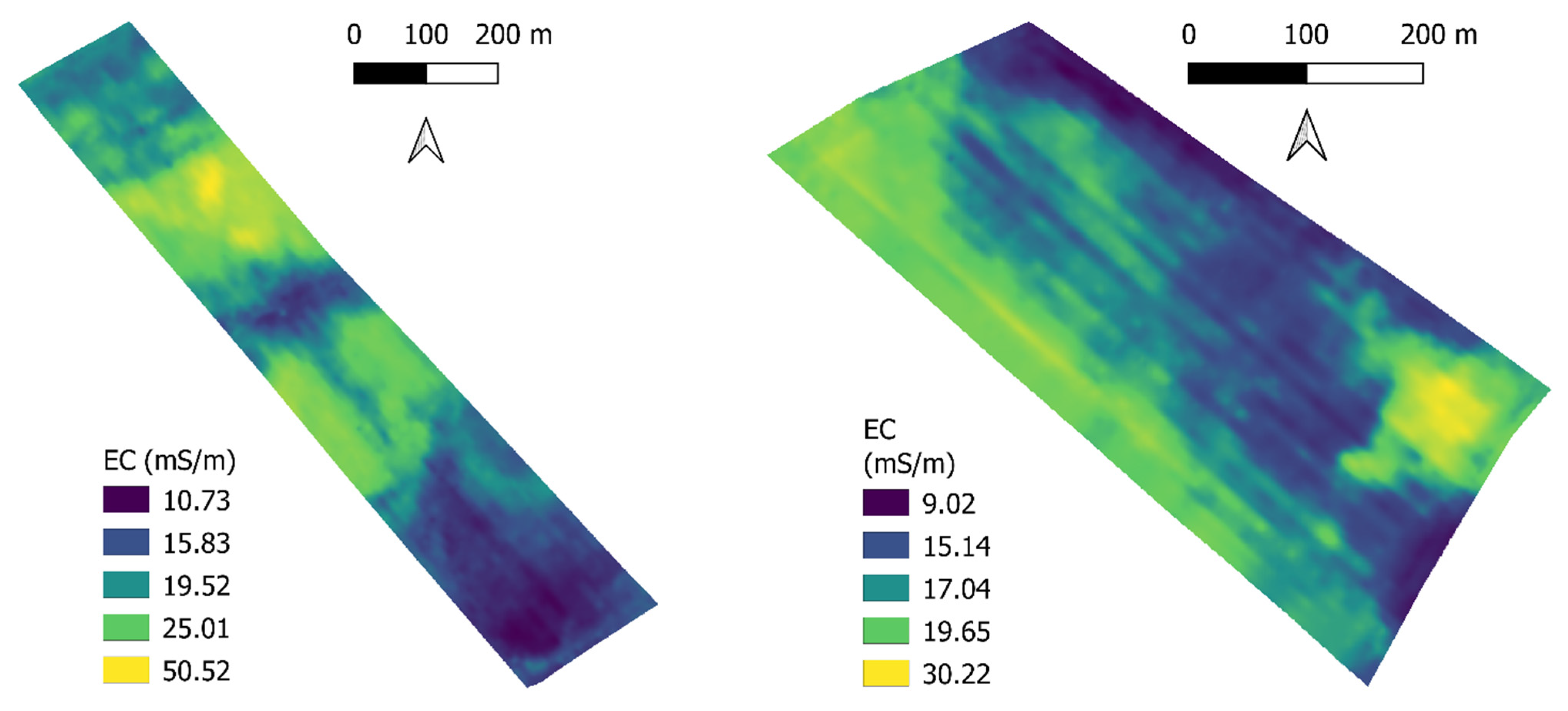
The soil spatial variability was detected by means of low induction electromagnetic technique of CMD miniexplorer (GF Instruments, s.r.o., Brno, Czech Republic) with 6 m between transects and an average measurement distance of 0.8 m along transects.

The CMD miniexplorer returns data must be interpolated; in this case, the inverse distance squared method was performed by using Qgis [29,30,31].

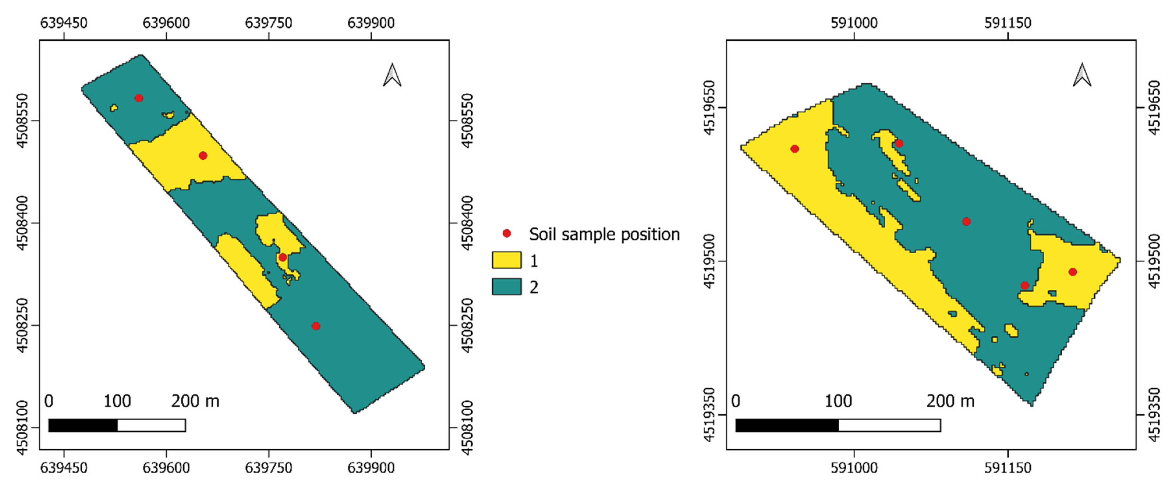
After obtaining the electrical resistivity map, the cluster analysis was performed to identify the zones, and then for each zone, soil samples at the depths of 0–40 cm were collected and characterized by conventional analytical methods according to [32]. All samples were air-dried, and 2-mm sieved before laboratory analyses.

The organic carbon (OC) content was measured by the Walkley–Black method, and the total Kjeldahl nitrogen was determined by the Kjeldahl method. The available phosphorus (Pava) was determined by ultraviolet and visible (UV–vis) spectrophotometry according to the Olsen method. The total content of CaCO₃ was determined by the gas-volumetric methods (Freuling calcimeter method), whereas the active lime was extracted with 0.1 M ammonium oxalate and determined by titration with 0.1 M KMnO₄.

At crop maturity, the grain yield (t ha⁻¹) and protein content (%) was measured on a sample area of 4 m² replicated three times. The protein content (%) was measured by the FOSS Infratec 1241.

2.3. Management Zone Delineation Approach

The management zones map creation workflow was entirely performed with R statistical software [33]. The workflow to generate the management zone map is composed of several steps, which could be summarized as (1) import resistivity map, (2) raster to dataframe conversion, (3) cluster analysis, (4) management zone map creation and (5) export.

The resistivity maps were imported to R by using the “raster” function of the raster R package [34]. After checking the geographical reference system and the spatial resolution, the resistivity maps were converted to “dataframe” R object by using the “as.data.frame” function of the raster R package.

The cluster analysis was performed by using the “kmeans” function of the stats R package [33]. The “kmeans” function requires the number of “centers” as a mandatory parameter, which defines the number of clusters that the algorithm must perform.

The optimal number of “centers” was defined by performing the gap statistic index, which calculates the goodness of clustering by comparing the total intra-cluster variation for different values of k with their expected values under the null reference distribution of the data. The gap statistic index was performed by using the “clusGap” function of the cluster R package [35].

Based on the gap statistic index, the k-means cluster analysis was performed, and the zone management map was created and converted to the spatialpolygonsdataframe R object by using the “df_to_SpatialPolygons” function of the FRK package [36]. The spatialpolygonsdataframe was exported by using the “writeOGR” function of the rgdal R package [37] in an ESRI Shapefile file format.

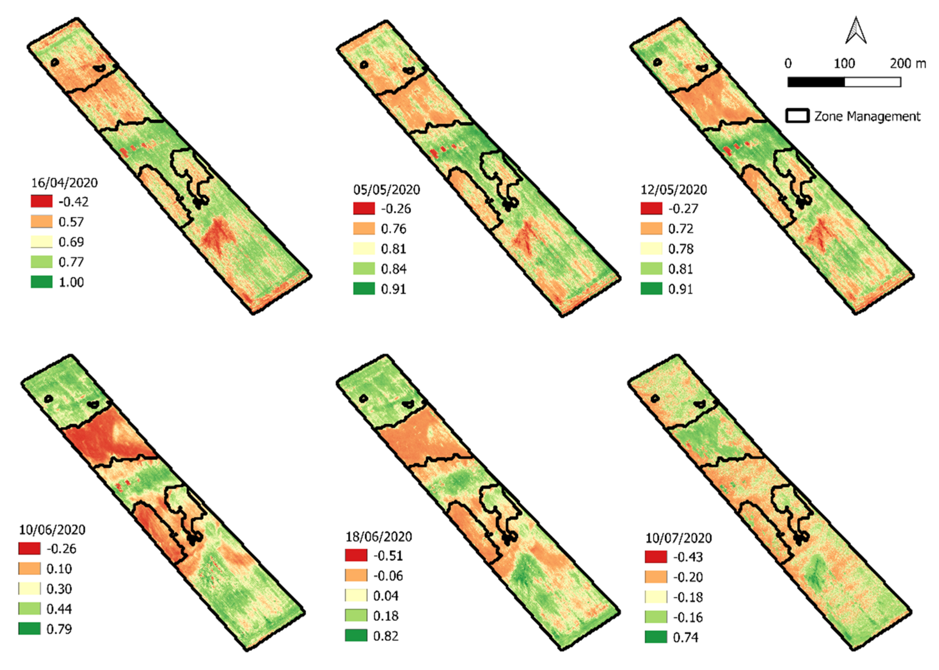
2.4. UAV Images Acquisition

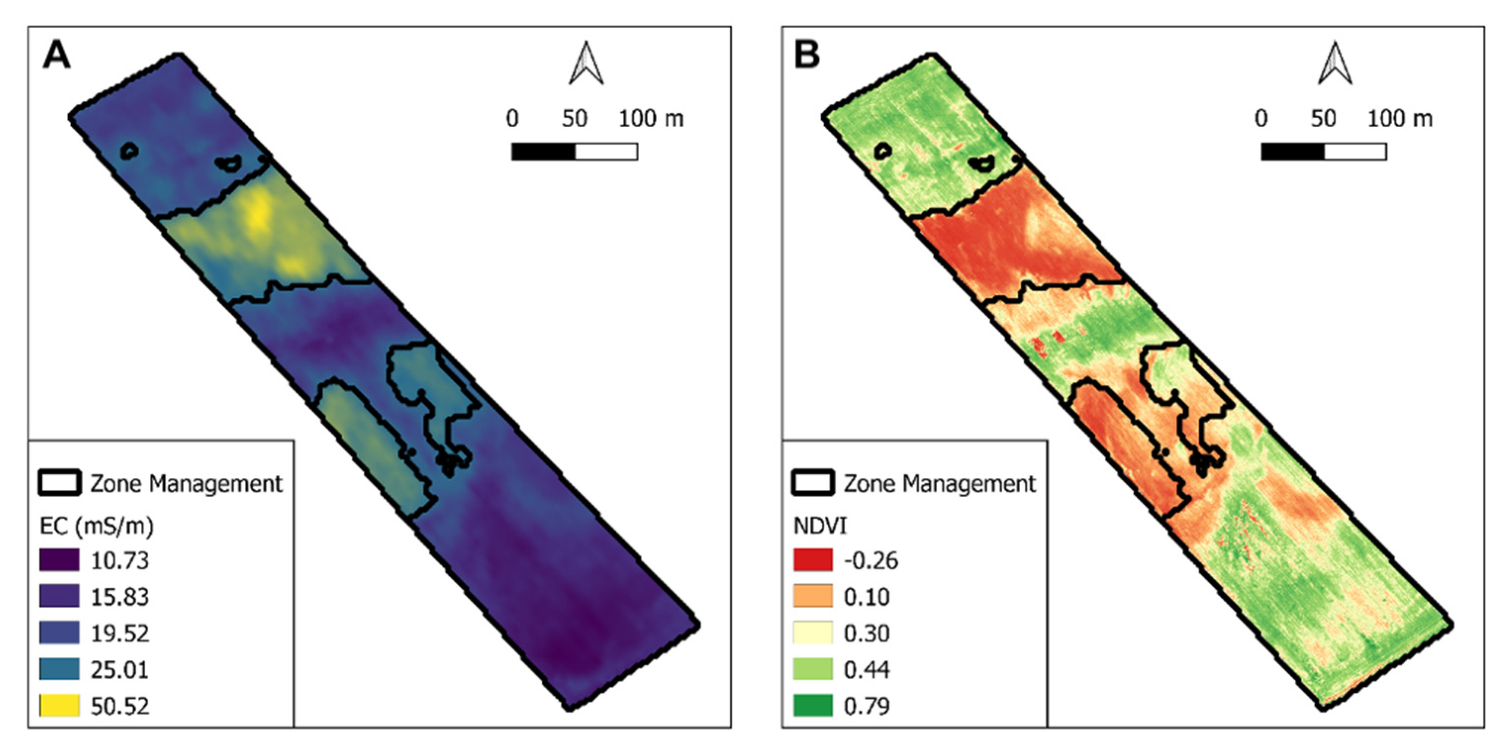
The UAV images acquisition was conducted in 2019–2020 at site 1. The images were acquired using a Parrot Bluegrass drone with a Parrot Sequoia multispectral sensor, and the flight plan was set using Pix4Dcapute. Six flight missions were carried out throughout the durum wheat crop cycle (

Table 3. Flight missions date (dd mm yyyy) and relative phenological stages.

Date	Phenological State
16 April 2020	Advanced tillering
5 May 2020	Beginning of stem elongation
12 May 2020	Advanced booting
10 June 2020	Inflorescence emergence
18 June 2020	Anthesis
10 July2020	Maturity

).

For the agriculture domain sector, each image acquired by UAV flight required an image processing workflow to compute the vegetation index (VI). The image processing is composed of three main steps: (1) orthomosaic reflectance map generation; (2) computation of VI maps; (3) data extraction.

Starting from the raw tiff files acquired by the UAV, the orthomosaic reflectance map was generated by using structure from motion (SfM) software [38], which in this case was PIX4D.

In order to complete the second main step, the orthomosaic reflectance map was imported in R statistical software [33], and the VI shown in

Table 4. Vegetation indexes formulas and references.

Vegetation Index	Formula	References
MSAVI2	$\mathrm{MSAVI}2=\frac{2\ast \mathrm{NIR}+1-\sqrt{{\left(2\ast \mathrm{NIR}+1\right)}^2-8\left(\mathrm{NIR}-\mathrm{Red}\right)}}{2}$	[40]
NDRE	$\mathrm{NDRE}=\frac{\mathrm{NIR}-\mathrm{Red}\mathrm{Edge}}{\mathrm{NIR}+\mathrm{Red}\mathrm{Edge}}$	[41]
NDVI	$\mathrm{NDVI}=\frac{\mathrm{NIR}-\mathrm{Red}}{\mathrm{NIR}+\mathrm{Red}}$	[42]
EVI2	$\mathrm{EVI}2=2.5\ast \frac{\mathrm{NIR}-\mathrm{Red}}{\mathrm{NIR}+\left(2.4\ast \mathrm{Red}\right)+1}$	[43]
WV.VI	$\mathrm{WV}.\mathrm{VI}=\frac{{\mathrm{NIR}}^2-\mathrm{Red}}{{\mathrm{NIR}}^2+\mathrm{Red}}$	[44]

was calculated [39].

In order to define the relationship between the previous VI and the resistivity map, the coefficient of determination (R²) was computed. (1) The VI maps were scaled at the same resolution as the resistivity map by using the “resample” function of the raster R Package [34]. (2) After obtaining raster files with the same resolution, they were converted to a data frame by using the “as.data.frame” function of the raster R Package [34]. (3) Then, a linear model was fitted by using the “lm” function of the stats R Package [33] in order to compute the R².

2.5. Statistical Analysis

All the statistical analyses were performed with R statistical software [33].

Before performing any analysis, a descriptive statistics analysis was performed on the resistivity maps; the range and the coefficient of variation (CoV) to describe the spatial variability of both sites were calculated.

In order to validate the zone management map creation workflow, the statistical analysis was performed on the soil samples, which were assigned an experimental factor in relation to the zone management area previously defined.

In order to perform the statistical analysis, a one-factor linear model was built by using the “lm” function of the stats R package [33], on which the cluster was considered the main factor.

Before performing the Analysis of Variance (ANOVA), whether the model met the three assumptions of the ANOVA was verified [45]. The Normality distribution of the model residual was checked both graphically (QQ-plot) and by performing the Shapiro–Wilk normality test. Moreover, the homoscedasticity was checked using the Levene test. The last ANOVA assumption was satisfied by the experimental design and the random sampling.

When all the three ANOVA assumptions were met, the ANOVA was applied to the model. Only when the ANOVA showed a significant difference (p-value < 0.05), the estimated marginal means post hoc analysis was performed by using the “emmeans” function with the Bonferroni adjustment of the emmeans R package [46].

For the yield dataset, the same procedure of the soil samples dataset was performed, except that the statistical analysis was performed on a full factorial model where the site and zone management were set as experimental factors.

3. Results

3.1. Resistivity Maps

The resistivity maps of both sites are shown in Figure 3. The values were scaled based on quartiles to show the in-field spatial variability better. Based on the previous scale classification, both sites showed high spatial variability. As evidence of the different spatial variability, both range and coefficient of variation (CoV) were calculated (

Table 5. Descriptive statistics of EC for both sites.

Site	EC
	Mean	Dev Std	CoV 1	Min	Max	Range
1	21.40	7.28	34.02	11.00	51.00	39.76
2	17.50	3.31	18.91	9.00	30.00	21.20

¹ CoV: Coefficient of variation.

). The first site obtained a higher value of +15.11 CoV and +18.56 of range than the second site. While considering the EC value, the first site obtained a higher value of +3.90 mS m⁻¹ than the second site (Table 5).

3.2. Zone Management Delineation and Statistical Analysis Results

The number of the optimal “centers” to associate as a parameter for the k-means computation was defined based on the gap statistic index. For both sites, the gap statistic index defined that the optimal number of clusters was two. The zone management map visualization is reported in Figure 4.

In order to agronomically validate the two zones identified by the k-means classification for both sites, we set an experimental factor of the soil samples based on the affiliation of zone management. Then the zone management experimental factor was analyzed by the ANOVA applied to the soil sample.

The ANOVA showed that the zone management defined by the k-means was statistically significant for clay, silt, bulk density, EC, organic matter, organic carbon, total carbonate, nitrogen and ratio C/N for both sites (

Table 6. Results of the ANOVA applied to the soil samples based on the zone management experimental factor for both sites.

Site	Factor	Df 1	Clay	Silt	Sand	Bulk Density
1	ZM 2	1	*	*	0.98	*
2	ZM	1	*	*	*	*

¹ df: Degree of freedom; ² ZM: Zone management; *: Significant at p < 0.05%.

,

Table 7. Results of the ANOVA applied to the soil samples based on the zone management experimental factor for both sites.

Site	Factor	Df 1	EC 2	Organic Matter	Organic Carbon	Totale Carbonetes	Nitrogen	C/N 3
1	ZM 4	1	*	*	*	*	*	*
2	ZM	1	*	*	*	*	*	*

¹ df: Degree of freedom; ² EC: Electrical conductivity; ³ C/N: Ratio carbon–nitrogen; ⁴ ZM: Zone management; *: Significant at p < 0.05%.

and

Table 8. Results of the ANOVA applied to the soil samples based on the zone management experimental factor for both sites.

Site	Factor	Df 1	Mg/K 2	Na	Mg	P	AWC 3	pH
1	ZM 4	1	0.27	0.4	0.27	0.52	0.96	0.97
2	ZM	1	0.9	0.11	*	0.14	0.34	0.72

¹ df: Degree of freedom; ² Mg/K: Ratio Magnesium potassium; ³AWC: Available water content; ⁴ ZM: Zone management; *: Significant at p < 0.05%.

).

In addition to the variables previously cited, for the second site, the ANOVA showed a statistical impact of zone management for sand and magnesium (Table 6, Table 7 and Table 8). However, the ANOVA did not show a statistical impact of the zone management for the ratio Mg/K, sodium, phosphorus, AWC and pH.

The emmeans with the Bonferroni adjustment analysis showed that, for both sites, zone number 2 obtained a statistically higher value than zone number 1 for clay, EC, organic matter, organic carbon, nitrogen and ratio C/N. However, no statistical superiority was highlighted between the two zones of both sites for Mg/K, phosphorus, AWC and pH (

Table 9. Results of the emmeans function applied to the soil samples based on the zone management experimental factor for both sites.

Site	ZM 1	Clay		Silt		Sand		Bulk Density		EC 2		Organic Matter		Organic Carbon		Total Carbonates
		Mean	Dev Std	Mean	Dev Std	Mean	Dev Std	Mean	Dev Std	Mean	Dev Std	Mean	Dev Std	Mean	Dev Std	Mean	Dev Std
1	1	33.80 b	3.11	43.05 a	8.56	23.15 a	11.67	1.36 a	0.01	0.17 b	0.04	1.62 b	0.06	0.94 b	0.04	35.62 a	2.24
	2	41.70 a	2.55	35.45 b	0.64	22.85 a	1.91	1.28 b	0.02	0.11 a	0.06	2.39 a	0.25	1.39 a	0.15	26.97 b	2.23
2	1	27.00 b	11.31	27.00 b	2.83	46.00 a	14.14	1.42 a	0.09	0.19 b	0.04	1.03 b	0.71	0.60 b	0.41	20.65 a	12.52
	2	37.67 a	3.06	33.33 a	3.21	29.00 b	2.65	1.32 b	0.02	0.23 a	0.01	1.92 a	0.24	1.12 a	0.14	15.20 b	9.61

¹ ZM: Zone management; ² EC: Electrical conductivity. Means within column that are followed by the same letter are not significantly different at p < 0.05%.

and

Table 10. Results of the emmeans function applied to the soil samples based on the zone management experimental factor for both sites.

Site	ZM 1	Nitrogen		C/N 2		Mg/K 3		Na		Mg		P		AWC 4		pH
		Mean	DEV Std	Mean	Dev Std	Mean	Dev Std	Mean	Dev Std	Mean	Dev Std	Mean	Dev Std	Mean	DEV Std	Mean	Dev Std
1	1	1.50 b	0.04	6.25 b	0.35	1.26 a	0.06	0.06 a	0.01	0.83 a	0.02	10.00 a	2.83	147.5 a	12.02	8.35 a	0.07
	2	1.79 a	0.05	7.75 a	0.64	3.46 a	1.57	0.14 a	0.11	2.57 a	1.61	12.50 a	3.54	148.00 a	5.07	8.35 a	0.07
2	1	0.66 b	0.37	8.76 b	1.25	4.13 a	1.56	0.20 b	0.04	2.08 b	0.35	6.50 a	0.71	85.50 a	7.78	8.20 a	0.14
	2	1.18 a	0.06	9.41 a	0.74	3.96 a	1.07	0.60 a	0.23	3.67 a	0.34	9.00 a	1.73	94.33 a	9.02	8.17 a	0.06

¹ ZM: Zone management; ² C/N: Ratio carbon–nitrogen; ³ Mg/K: Ratio Magnesium potassium; ⁴ AWC: Available water content. Means within column that are followed by the same letter are not significantly different at p < 0.05%.

).

Furthermore, for site 1, zone 2 obtained a higher percentage value of +18.95% of clay, +35.29 % of EC, +32.22% of organic matter, +32.37% of organic carbon, +16.20% of nitrogen and +19.35% ratio C/N than the zone 1. While zone 1 obtained a higher percentage value of +17.65 of silt, +5.88 % bulk density and +24.28% of total carbonates than zone 2 (Table 9 and Table 10).

For site 2, zone 2 resulted statistically superior for +28.32% of clay, +18.99% of silt, +17.39% of EC, +46.35% of organic matter, +46.43% of organic carbon, +44.07% of nitrogen, +6.91% of ration C/N and +66.67% of sodium than zone 1 (Table 7 and Table 8). However, zone 1 showed a statistically higher for +36.96% of sand, +7.04% of bulk density and +26.39% of total carbonates than zone 2.

Based on the results obtained above, it can be stated that zone 2 generated by the cluster analysis for both sites has soil physical and chemical characteristics superior to zone 1 for durum wheat cultivation, such as higher clay, silt, EC, organic matter, organic carbon, nitrogen and the ratio of carbon and nitrogen.

3.3. Grain Yield and Statistical Analysis

The ANOVA applied to the full factorial model showed that the single effect of site and zone management statistically impacts the grain yield (t/ha) and grain protein content (%). Moreover, the combined effect of the interaction between site and zone management statistically impacted the grain yield (t/ha), while for the protein content, no statistical impact was raised (

Table 11. Results of the ANOVA applied to the grain yield and protein content on the zone management experimental factor for both sites.

Experimental Factor	Df 1	Grain Yield (t/ha)	Protein (%)
		p Value	p Value
Site	1	***	***
ZM 2	1	*	***
Site × Zone	1	***	0.11

¹ df: Degree of freedom; ZM: Zone management; *: Significant at p < 0.05%; ***: Significant at p < 0.001%.

). Since we observed a significant difference in the combined effect, we applied the post hoc analysis on the site and zone management interaction.

With reference to the production (grain yield t/ha), the ML approach shows for both sites 1 and 2, and for both fertilization application N (UA) and N (VRT) a difference between management zones 1 and 2 (

Table 12. Results of the emmeans function applied to the grain yield and protein content based on the zone management experimental factor for both sites.

N	Approach	Zones	Site 1		Site 2
			Grain Yield t ha−1	Protein %	Grain Yield t ha−1	Protein %
			Mean	Mean	Mean	Mean
UA	ZH	c	5.2 b	14.1 a	1.7 b	12.9 b
		b	6.0 a	12.2 b	3.1 a	15 a
		a	6.3 a	12.4 b	3.2 a	13.3 b
	ML	1	5.2 b	14.1 a	1.7 b	12.9 b
		2	6.15 a	12.3 b	3.1 a	14.2 a
VRT	ZH	c	4.8 b	13.7 a	1.8 b	13.6 b
		b	5.6 a	12 b	2.9 a	16.4 a
		a	5.5 a	13. 2 a	3.2 a	14.6 b
	ML	1	4.8 b	13.7 a	1.8 b	13.6 b
		2	5.5 a	12.6 b	3.05 a	15.5 a

Means within column that are followed by the same letter are not significantly different at p < 0.05%.

). Specifically, in site 1 in N (UA), zone 2 shows the production of +0.95 t/ha with respect to zone 1; in zone 2 in N (VRT), it produced +0.7 t/ha with respect to zone 1.

Furthermore, in site 2 in N (UA), zone 2 produced + 1.4 t/ha with respect to zone 1; in N (VRT), zone 2 produced + 1.25 t/ha with respect to zone 1 (Table 12). The same is true for the % of grain proteins content where the difference is relevant for both site 1 and site 2 between management zones 1 and 2 defined with ML.

In line with the results described, it is possible to underline that in the ZH approach for both sites with reference to production (grain yield t/ha), even considering the N (UA) and N (VRT) treatments, a significant difference is highlighted between zone c with respect to zones a b. This reinforces the results obtained from the test of the approach (ML) as zones a b flow into zone 2, and zone c flows into zone 1 (Table 12).

3.4. Relationship between Vegetation Index and Resistivy Map

Six UAV flight missions were performed during all growing seasons in site 1 to obtain multispectral images to compute five vegetation indexes and evaluate the relationship with the resistivity map. As reported in

Table 13. Coefficient of determination (R²) of the relationship between the vegetation indexes and the resistivity map during all growing seasons.

Vegetation Index	Date
	16 April 2020	5 May 2020	12 May 2020	10 June 2020	18 June 2020	10 July 2020
NDRE	0.05	0.01	0.04	0.52	0.28	0.03
NDVI	0.02	0.01	0.08	0.56	0.35	0.02
MSAVI2	0.02	0.01	0.07	0.55	0.30	0.01
EVI2	0.02	0.01	0.06	0.55	0.31	0.01
WV.VI	0.03	0.02	0.11	0.45	0.23	0.01

, the coefficient of determination of the relationship between the vegetation indexes and the resistivity map is not significant until flowering.

During flowering, the maximum value of correlation is reached with an average coefficient of determination of 0.53. After flowering, the correlation value decreases for each vegetation indexes until the maturity of the durum wheat, where a non-significant correlation is shown (Table 13). The vegetation index that showed a higher relationship with the resistivity map is the NDVI [40], which reached an R² of 0.56 during flowering, while the vegetation index that reported the lowest R² was the WV.VI.

The NDVI maps are reported in Figure 5, which were scaled by using the quartile and where it is possible to appreciate the evolution of the NDVI throughout the year. All the NDVI maps were scaled by using the quartile. While in Figure 6, it is possible to appreciate the overlapping of the resistivity map, NDVI and the zone management defined by the cluster analysis.

4. Discussion

4.1. Soil Sensor and Management Zone Creation

Proximal soil sensors are receiving strong attention from several disciplinary fields, and this has led to a rise in the number of proximal soil sensors available in the market in the last two decades [47]. These sensors contribute to measuring the spatial-temporal variability of soil proprieties, such as moisture content and soil texture [48].

These sensors could be used to measure the soil organic matter, nitrogen availability and the ratio of carbon–nitrogen indirectly, which are soil variables that are mostly considered to calculate the nitrogen balance in several integrated production standards [49]. Moreover, after careful evaluation and calibration, these sensors can avoid time-consuming and expensive soil sampling and analysis, which cannot be scaled at the farm level [50].

Based on previous assumptions, it is essential to use the proximal soil sensor in order to characterize the soil proprieties and to perform the SSNM (Site-Specific Nitrogen Management) [19].

By using the EMI sensor, we could generate the resistivity map, which can be used as the information layer to define the zone management. Different approaches such as the multivariate geostatistical approach [51] or the machine learning approach were found in the literature, which deal well with non-linear patterns [27,52].

Our contribution is to validate agronomically the k-means algorithm to delineate zone management which uses the resistivity map by using a statistical approach. Both sites under study showed a different spatial variability which allowed us to validate the approach in two different field conditions. The unsupervised machine learning algorithm, which was the k-means [53] based on the gap statistic index [35], reported the existence of two zone managements at both sites.

At both sites, multiple soil and crop samples were performed in those different zones in order to perform a statistical analysis to agronomically validate the presence of the two zones [54]. At both sites, between the two zones, there was a significant difference in clay (%), silt (%), bulk density (g m⁻³), EC (mS m⁻¹) organic matter (%), organic carbon (%), total carbonates (%), nitrogen (g kg⁻¹) and C/N.

The second zone for both sites showed a higher value of organic matter, organic carbon, nitrogen and ratio of nitrogen and carbon, which led to higher grain yield (t ha⁻¹) than the first zone. This result is in accordance with [55], where a higher content of soil organic matter and nitrogen led to a higher value of several vegetation indexes and grain yield (t ha⁻¹). Moreover, it was observed that the differences in yield are significant between zones and not within zones. While for the grain protein content (%), the difference was found only in the two sites where the resistivity map obtained a higher spatial variability.

4.2. Relationship between Vegetation Indexes and Resistivity Map

Efficient and reliable methods for measuring spatial variability in soil properties are fundamental in precision agriculture [56].

It is by using these instruments precisely that spatial variability can be estimated without soil sampling, which is time–money consuming [50].

Beyond the use of proximal soil sensors, several authors tried to use remote sensing data, such as Sentinel-2 multispectral images, in order to predict the spatial soil proprieties, such as organic carbon [57] and electrical conductivity [58]. Other authors tried the Pedotransfer Functions [59] or neural networks [60] in order to improve the accuracy of the models.

We showed that the correlation between the VI and the resistivity map depends strongly on the phenological and developmental stage of the durum wheat. During the whole development of the crop, there is no significant correlation, except during flowering when the linear correlation reaches 0.53 of the R².

This is because flowering is the most important and susceptible phase of crop phenological development. During flowering, the crop reaches its maximum development, generating maximum leaf development.

It is at that point that differences in nitrogen uptake due to soil differences are shown in the crop [5].

Moreover, NDVI was the best vegetation index to be related to the resistivity map, while the worst VI was the WV.VI.

5. Conclusions

Two sites were mapped through an electromagnetic induction sensor to measure the electric conductivity map. An unsupervised machine learning approach was applied to the resistivity maps to detect the presence of different zones. Based on the results of the classification algorithm, multiple soil and crop samples were taken to validate the difference of the zones agronomically.

The algorithm used was able to detect the presence of the two zones for both sites. The soil samples acquired showed a significant difference between zones and not within zones for organic matter, nitrogen and the ratio of carbon–nitrogen. The differences reported on the soil proprieties led to a statistical difference in the grain yield obtained between the zones detected by the k-means algorithm.

This approach could be used to provide a high-quality prescription map to apply the precision agriculture applications. This approach could be scaled at the farm level; one resistivity survey and a few soil samples could generate a high-quality prescription map, containing costs and falling within the farm-year budget. Future work will focus on creating an automated nitrogen fertilization determination method starting from the acquired soil data.

Moreover, the correlation between the VI and resistivity map depends strongly on the phenological and developmental stage of the durum wheat. Therefore, we suggest performing the UAV multispectral images acquisition during the flowering phenological stages to attribute the crop spatial variability to different soil conditions.

References

1. Guerrini, L.; Napoli, M.; Mancini, M.; Masella, P.; Cappelli, A.; Parenti, A.; Orlandini, S. Wheat Grain Composition, Dough Rheology and Bread Quality as Affected by Nitrogen and Sulfur Fertilization and Seeding Density. Agronomy 2020, 10, 233. [Google Scholar] [CrossRef] [Green Version]
2. Corwin, D.L. Past, Present, and Future Trends in Soil Electrical Conductivity Measurements Using Geophysical Methods; CRC Press; Taylor & Francis Group: New York, NY, USA, 2008. [Google Scholar]
3. Mulla, D.J.; McBratney, A.B. Soil spatial variability. In Soil Physics Companion; CRC Press: Boca Raton, FL, USA, 2001; pp. 343–373. [Google Scholar]
4. Buttafuoco, G.; Castrignanò, A.; Colecchia, A.S.; Ricca, N. Delineation of Management Zones Using Soil Properties and a Multivariate Geostatistical Approach. Ital. J. Agron. 2010, 5, 323–332. [Google Scholar] [CrossRef] [Green Version]
5. Fiorentini, M.; Zenobi, S.; Orsini, R. Remote and Proximal Sensing Applications for Durum Wheat Nutritional Status Detection in Mediterranean Area. Agriculture 2021, 11, 39. [Google Scholar] [CrossRef]
6. Mouazen, A.; Alexandridis, T.; Buddenbaum, H.; Cohen, Y.; Moshou, D.; Mulla, D.; Nawar, S.; Sudduth, K.A. Monitoring. In Agricultural Internet of Things and Decision Support for Precision Smart Farming; Elsevier Inc.: Amsterdam, The Netherlands, 2020; pp. 35–138. [Google Scholar]
7. Corwin, D.L.; Lesch, S.M. Application of Soil Electrical Conductivity to Precision Agriculture. Agron. J. 2003, 95, 455–471. [Google Scholar] [CrossRef]
8. Sudduth, K.A.; Kitchen, N.R.; Bollero, G.A.; Bullock, D.G.; Wiebold, W.J. Comparison of Electromagnetic Induction and Direct Sensing of Soil Electrical Conductivity. Agron. J. 2003, 95, 472–482. [Google Scholar] [CrossRef]
9. Doolittle, J.A.; Brevik, E.C. The use of electromagnetic induction techniques in soils studies. Geoderma 2014, 223–225, 33–45. [Google Scholar] [CrossRef] [Green Version]
10. Lark, R. Forming spatially coherent regions by classification of multi-variate data: An example from the analysis of maps of crop yield. Int. J. Geogr. Inf. Sci. 1998, 12, 83–98. [Google Scholar] [CrossRef]
11. Morari, F.; Castrignanò, A.; Pagliarin, C. Application of multivariate geostatistics in delineating management zones within a gravelly vineyard using geo-electrical sensors. Comput. Electron. Agric. 2009, 68, 97–107. [Google Scholar] [CrossRef]
12. Xin-Zhong, W.; Guo-Shun, L.; Hong-Chao, H.; Zhen-Hai, W.; Qing-Hua, L.; Xu-Feng, L.; Wei-Hong, H.; Yan-Tao, L. Determination of management zones for a tobacco field based on soil fertility. Comput. Electron. Agric. 2009, 65, 168–175. [Google Scholar] [CrossRef]
13. Brock, A.; Brouder, S.M.; Blumhoff, G.; Hofmann, B.S. Defining Yield-Based Management Zones for Corn-Soybean Rotations. Agron. J. 2005, 97, 1115–1128. [Google Scholar] [CrossRef] [Green Version]
14. Kitchen, N.; Sudduth, K.; Myers, D.; Drummond, S.; Hong, S. Delineating productivity zones on claypan soil fields using apparent soil electrical conductivity. Comput. Electron. Agric. 2005, 46, 285–308. [Google Scholar] [CrossRef]
15. Officer, S.; Kravchenko, A.; Bollero, G.; Sudduth, K.; Kitchen, N.; Wiebold, W.; Palm, H.; Bullock, D. Relationships between soil bulk electrical conductivity and the principal component analysis of topography and soil fertility values. Plant Soil 2004, 258, 269–280. [Google Scholar] [CrossRef]
16. Ortega, R.A.; Santibáñez, O.A. Determination of management zones in corn (Zea mays L.) based on soil fertility. Comput. Electron. Agric. 2007, 58, 49–59. [Google Scholar] [CrossRef]
17. Rossi, R.; Pollice, A.; Bitella, G.; Bochicchio, R.; D’Antonio, A.; Alromeed, A.A.; Stellacci, A.M.; Labella, R.; Amato, M. Soil bulk electrical resistivity and forage ground cover: Nonlinear models in an alfalfa (Medicago sativa L.) case study. Ital. J. Agron. 2015, 10, 215–219. [Google Scholar] [CrossRef] [Green Version]
18. Pollice, A.; Lasinio, G.J.; Rossi, R.; Amato, M.; Kneib, T.; Lang, S. Bayesian measurement error correction in structured additive distributional regression with an application to the analysis of sensor data on soil–plant variability. Stoch. Environ. Res. Risk Assess. 2019, 33, 747–763. [Google Scholar] [CrossRef] [Green Version]
19. Fridgen, J.J.; Kitchen, N.R.; Sudduth, K.A.; Drummond, S.T.; Wiebold, W.J.; Fraisse, C.W. Management zone analyst (MZA): Software for subfield management zone delineation. Agron. J. 2004, 96, 100–108. [Google Scholar] [CrossRef]
20. Schepers, A.R.; Shanahan, J.F.; Liebig, M.A.; Schepers, J.S.; Johnson, S.H.; Luchiari, A. Appropriateness of Management Zones for Characterizing Spatial Variability of Soil Properties and Irrigated Corn Yields across Years. Agron. J. 2004, 96, 195–203. [Google Scholar] [CrossRef] [Green Version]
21. Khosla, R. Precision agriculture: Challenges and opportunities in a flat world. In Proceedings of the 19th World Congress of Soil Science, Soil Solutions for a Changing World, Brisbane, Australia, 1–6 August 2010. [Google Scholar]
22. Aggelopooulou, K.; Castrignanò, A.; Gemtos, T.; De Benedetto, D. Delineation of management zones in an apple orchard in Greece using a multivariate approach. Comput. Electron. Agric. 2013, 90, 119–130. [Google Scholar] [CrossRef]
23. Buttafuoco, G.; Castrignanò, A.; Cucci, G.; Rinaldi, M.; Ruggieri, S. An approach to delineate management zones in a durum wheat field: Validation using remote sensing and yield mapping. Precis. Agric. 2015, 15, 241–248. [Google Scholar]
24. Kitchen, N.R.; Snyder, C.J.; Franzen, D.W.; Wiebold, W.J. Educational Needs of Precision Agriculture. Precis. Agric. 2002, 3, 341–351. [Google Scholar] [CrossRef]
25. Mzuku, M.; Khosla, R.; Reich, R.; Inman, D.; Smith, F.; Macdonald, L. Spatial Variability of Measured Soil Properties across Site-Specific Management Zones. Soil Sci. Soc. Am. J. 2005, 69, 1572–1579. [Google Scholar] [CrossRef] [Green Version]
26. Castrignanò, A.; Buttafuoco, G.; Quarto, R.; Parisi, D.; Rossel, R.V.; Terribile, F.; Langella, G.; Venezia, A. A geostatistical sensor data fusion approach for delineating homogeneous management zones in Precision Agriculture. Catena 2018, 167, 293–304. [Google Scholar] [CrossRef]
27. Gavioli, A.; de Souza, E.G.; Bazzi, C.L.; Schenatto, K.; Betzek, N. Identification of management zones in precision agriculture: An evaluation of alternative cluster analysis methods. Biosyst. Eng. 2019, 181, 86–102. [Google Scholar] [CrossRef]
28. Moshou, D.; Bravo, C.; Wahlen, S.; West, J.; McCartney, A.; De Baerdemaeker, J.; Ramon, H. Simultaneous identification of plant stresses and diseases in arable crops using proximal optical sensing and self-organising maps. Precis. Agric. 2006, 7, 149–164. [Google Scholar] [CrossRef]
29. QGIS Development Team. QGIS Geographic Information System. 2009. Available online: http://qgis.org (accessed on 15 December 2021).
30. Kumar, G.M.; Priyadarshini, R. Electrical Conductivity Sensing for Precision Agriculture: A Review BT. In Harmony Search and Nature Inspired Optimization Algorithms: Theory and Applications, ICHSA 2018; Springer: Singapore, 2019; pp. 647–659. [Google Scholar]
31. Minasny, B.; Berglund, Ö.; Connolly, J.; Hedley, C.; de Vries, F.; Gimona, A.; Kempen, B.; Kidd, D.; Lilja, H.; Malone, B.; et al. Digital mapping of peatlands—A critical review. Earth-Sci. Rev. 2019, 196, 102870. [Google Scholar] [CrossRef]
32. Blume, H.-P.; Page, A.L.; Miller, R.H.; Keeney, D.R. Methods of soil analysis; 2. Chemical and microbiological properties, 2. Aufl. 1184 S.; American Soc. of Agronomy (Publ.), Madison, Wisconsin, USA, gebunden 36 Dollar. J. Plant Nutr. Soil Sci. 1985, 148, 363–364. [Google Scholar] [CrossRef]
33. R Foundation for Statistical Computing. A Language and Environment for Statistical Computing; R Foundation for Statistical Computing: Vienna, Austria, 2018; Volume 2, Available online: http://www.r-project.org (accessed on 15 December 2021).
34. Hijmans, R.J.; van Etten, J.; Sumner, M.; Cheng, J.; Baston, D.; Bevan, A.; Bivand, R.; Busetto, L.; Canty, M.; Fasoli, B.; et al. Raster: Geographic Data Analysis and Modeling. R package, Version 3.5-11. 2011. Available online: https://cran.r-project.org/web/packages/raster/raster.pdf (accessed on 15 December 2021).
35. Tibshirani, R.; Walther, G.; Hastie, T. Estimating the number of clusters in a data set via the gap statistic. J. R. Stat. Soc. Ser. B Stat. Methodol. 2001, 63, 411–423. [Google Scholar] [CrossRef]
36. Zammit-Mangion, A.; Cressie, N. FRK: An R Package for Spatial and Spatio-Temporal Prediction with Large Datasets. J. Stat. Softw. 2021, 98, 1–48. [Google Scholar] [CrossRef]
37. Bivand, R.; Keitt, T.; Rowlingson, B. Rgdal: Bindings for the Geospacial Data Abstraction Library. 2013. Available online: http://cran.r-project.org/package=rgdal (accessed on 15 December 2021).
38. Verhoeven, G. Taking computer vision aloft—Archaeological three-dimensional reconstructions from aerial photographs with photoscan. Archaeol. Prospect. 2011, 18, 67–73. [Google Scholar] [CrossRef]
39. Xue, J.; Su, B. Significant Remote Sensing Vegetation Indices: A Review of Developments and Applications. J. Sensors 2017, 2017, 1353691. [Google Scholar] [CrossRef] [Green Version]
40. Leprieur, C.; Kerr, Y.H.; Mastorchio, S.; Meunier, J.C. Monitoring vegetation cover across semi-arid regions: Comparison of remote observations from various scales. Int. J. Remote Sens. 2010, 21, 281–300. [Google Scholar] [CrossRef]
41. Barnes, E.M.; Clarke, T.R.; Richards, S.E.; Colaizzi, P.D.; Haberland, J.; Kostrzewski, M.; Waller, P.; Choi, C.; Riley, E.; Thompson, T.; et al. Coincident detection of crop water stress, nitrogen status and canopy density using ground based multispectral data. In Proceedings of the Fifth International Conference on Precision Agriculture, Bloomington, MN, USA, 16–19 July 2000; Volume 1619. [Google Scholar]
42. Rouse, J.W.; Haas, R.H.; Schell, J.A.; Deering, D.W. Monitoring vegetation systems in the Great Plains with ERTS. NASA Spec. Publ. 1974, 351, 309. [Google Scholar]
43. Jiang, Z.; Huete, A.; Kim, Y.; Didan, K. 2-band enhanced vegetation index without a blue band and its application to AVHRR data. In Proceedings of the PIE Conference on Optics + Photonics: SPIE Optical Engineering + Applications, San Diego, CA, USA, 26–30 August 2007; Volume 6679, p. 667905. [Google Scholar]
44. Wolf, A.F. Using WorldView-2 Vis-NIR multispectral imagery to support land mapping and feature extraction using normalized difference index ratios. In Algorithms and Technologies for Multispectral, Hyperspectral, and Ultraspectral Imagery XVIII; SPIE: Bellingham, WA, USA, 2012; Volume 8390, p. 83900N. [Google Scholar]
45. Onofri, A.; Seddaiu, G.; Piepho, H.-P. Long-Term Experiments with cropping systems: Case studies on data analysis. Eur. J. Agron. 2016, 77, 223–235. [Google Scholar] [CrossRef]
46. Lenth, R. Emmeans: Estimated Marginal Means Aka Least-Squares Means. 2019. Available online: https://cran.r-project.org/package=emmeans (accessed on 15 December 2021).
47. Mouazen, A.M.; Shi, Z.; Van Meirvenne, M. Sensing soil condition and functions. Biosyst. Eng. 2016, 152, 1–2. [Google Scholar] [CrossRef] [Green Version]
48. Heggemann, T.; Welp, G.; Amelung, W.; Angst, G.; Franz, S.O.; Koszinski, S.; Schmidt, K.; Pätzold, S. Proximal gamma-ray spectrometry for site-independent in situ prediction of soil texture on ten heterogeneous fields in Germany using support vector machines. Soil Tillage Res. 2017, 168, 99–109. [Google Scholar] [CrossRef]
49. Liu, Z.; Gao, J.; Gao, F.; Dong, S.; Liu, P.; Zhao, B.; Zhang, J. Integrated agronomic practices management improve yield and nitrogen balance in double cropping of winter wheat-summer maize. Field Crop. Res. 2018, 221, 196–206. [Google Scholar] [CrossRef]
50. Fiorentini, M.; Zenobi, S.; Giorgini, E.; Basili, D.; Conti, C.; Pro, C.; Monaci, E.; Orsini, R. Nitrogen and chlorophyll status determination in durum wheat as influenced by fertilization and soil management: Preliminary results. PLoS ONE 2019, 14, e0225126. [Google Scholar] [CrossRef]
51. Anastasiou, E.; Castrignanò, A.; Arvanitis, K.; Fountas, S. A multi-source data fusion approach to assess spatial-temporal variability and delineate homogeneous zones: A use case in a table grape vineyard in Greece. Sci. Total. Environ. 2019, 684, 155–163. [Google Scholar] [CrossRef]
52. Chlingaryan, A.; Sukkarieh, S.; Whelan, B. Machine learning approaches for crop yield prediction and nitrogen status estimation in precision agriculture: A review. Comput. Electron. Agric. 2018, 151, 61–69. [Google Scholar] [CrossRef]
53. MacQueen, J.B. Some methods for classification and analysis of multivariate observations. In Fifth Berkeley Symposium on Mathematical Statistics and Probability, Davis, CA, USA, 21 June–18 July 1965, 27 December 1965–7 January 1966; Statistical Laboratory of the University of California: Berkeley, CA, USA, 1967; Volume 1, pp. 281–297. [Google Scholar]
54. Gavioli, A.; Souza, E.G.; Bazzi, C.L.; Betzek, N.M.; Schenatto, K.; Beneduzzi, H. Delineation of site-specific management zones using spatial principal components and cluster analysis. In Proceedings of the SA13th International Conference on Precision Agriculture, St. Luis, MI, USA, 31 July–4 August 2016; pp. 1–11. [Google Scholar]
55. Orsini, R.; Fiorentini, M.; Zenobi, S. Evaluation of Soil Management Effect on Crop Productivity and Vegetation Indices Accuracy in Mediterranean Cereal-Based Cropping Systems. Sensors 2020, 20, 3383. [Google Scholar] [CrossRef]
56. Basso, B.; Dumont, B.; Cammarano, D.; Pezzuolo, A.; Marinello, F.; Sartori, L. Environmental and economic benefits of variable rate nitrogen fertilization in a nitrate vulnerable zone. Sci. Total Environ. 2016, 545–546, 227–235. [Google Scholar] [CrossRef] [PubMed] [Green Version]
57. Wang, H.; Zhang, X.; Wu, W.; Liu, H. Prediction of Soil Organic Carbon under Different Land Use Types Using Sentinel-1/-2 Data in a Small Watershed. Remote. Sens. 2021, 13, 1229. [Google Scholar] [CrossRef]
58. Pezzuolo, A.; Donato, C.; Marinello, F.; Sartori, L. Relationship between satellite-derived NDVI and soil electrical resis-tivity: A case study. In Proceedings of the 6th International Conference on Trends in Agricultural Engineering, Prague, Czech Republic, 7–9 September 2016; pp. 484–489. [Google Scholar]
59. Paul, S.; Coops, N.; Johnson, M.; Krzic, M.; Chandna, A.; Smukler, S. Mapping soil organic carbon and clay using remote sensing to predict soil workability for enhanced climate change adaptation. Geoderma 2020, 363, 114177. [Google Scholar] [CrossRef]
60. Schillaci, C.; Perego, A.; Valkama, E.; Märker, M.; Saia, S.; Veronesi, F.; Lipani, A.; Lombardo, L.; Tadiello, T.; Gamper, H.A.; et al. New pedotransfer approaches to predict soil bulk density using WoSIS soil data and environmental covariates in Mediterranean agro-ecosystems. Sci. Total. Environ. 2021, 780, 146609. [Google Scholar] [CrossRef]
Figure 1. Location of experimental sites.
Agronomy 12 00183 g001
Figure 2. Experimental site area visualization and relative soil sample position.
Agronomy 12 00183 g002
Figure 3. Resistivity map of the first site (Matera on the left) and of the second site (Genzano).
Agronomy 12 00183 g003
Figure 4. Zone management maps for both sites and relative soil samples position.
Agronomy 12 00183 g004
Figure 5. The NDVI maps reported for all growing seasons at site 1.
Agronomy 12 00183 g005
Figure 6. Overlapping of the resistivity map (A) and NDVI during flowering (B) and the zone management defined by the cluster analysis.
Agronomy 12 00183 g006