Artificial-Intelligence-Based Time-Series Intervention Models to Assess the Impact of the COVID-19 Pandemic on Tomato Supply and Prices in Hyderabad, India

Abstract

This study’s objective was to assess the impact of the COVID-19 pandemic on tomato supply and prices in Gudimalkapur market in Hyderabad, India. The lockdown imposed by the government of India from 25 March 2020 to 30 June 2020 particularly affected the supply chain of perishable agricultural products, including tomatoes as one of the major vegetable crops in the study area. The classical time series models such as autoregressive integrated moving average (ARIMA) intervention models and artificial intelligence (AI)-based time-series models namely support vector regression (SVR) intervention and artificial neural network (ANN) intervention models were used to predict tomato supplies and prices in the studied market. The modelling results show that the pandemic had a negative impact on supply and a positive impact on tomato prices. Moreover, the ANN intervention model outperformed the other models in both the training and test data sets. The superior performance of the ANN intervention model could be due to its ability to account for the nonlinear and complex nature of the data with exogenous intervention variable.

1. Introduction

Marketing is critical to moving agricultural products from producer to consumer and maintaining price stability. Changes in the demand and supply of agricultural products and marketing must be coordinated with projected increases in agricultural production. The COVID-19 crisis has caused significant damage to the national and global economy due to the lockdown measures initiated in March 2020 in many countries, including India. Due to the imposed lockdown, activities related to supply chains from the agriculture were notably disrupted and there was delayed of agricultural foodstuff. Tomatoes are the second most productive crop in the world after potatoes with a productivity of 32.8 t/ha. The major tomato producers in India are Andhra Pradesh, Madhya Pradesh, Karnataka, Gujarat, Odisha, and West Bengal. With a production of 2744.32 thousand tons, Andhra Pradesh is the state with the highest tomato production in India, followed by Madhya Pradesh with a production of 2419.28 thousand tons. Tomato is grown throughout the year in Telangana, which ranks seventh in India’s tomato production with a total area of over 41,000 hectares and production of 1171.5 tons [1]. Tomato is one of the major vegetable crops whose supply and price are affected by unexpected changes in government policies or other interventions.

Modelling and forecasting of supplies and prices helps in decision making and effective planning of the future for a developing economy and in determining the necessary policies for sustainable and overall development of the economy. Time series models are used to develop appropriate forecasting methods based on historical time series data of the variables under consideration. The autoregressive integrated moving average (ARIMA) model is extremely popular due to its statistical characteristics and well accepted Box–Jenkins methodology [2] for model building. Many researchers have used ARIMA models for time series forecasting of various agricultural commodities in the past, e.g., Naveena and others [3] for forecasting coconut production in India, Jalikatti and others [4,5] for forecasting onion prices and agricultural commodity prices; Kaur and others [6] used time series and SVR model for forecasting arrivals and process in Punjab. Rathod and others [7] applied an ARIMA genetic algorithm approach for predicting maize yield in India, while Rathod and others [8] used ARIMA and artificial intelligence (AI) techniques for predicting oilseed production in India. Tatarintsev and others [9] forecasted the prices of sugar using ARIMA model. In intervention time series modelling, ARIMA intervention [10] is the most commonly used model for forecasting time series in the context of interrupted time series. Earlier, ARIMA modelling with intervention was used in application planning and budgeting [11]. Ray and others [12] applied ARIMA intervention model to forecast cotton yield in India; and Ramasubramanian and Ray [13] applied ARIMA intervention model in power computation and they claimed that ARIMA intervention model was superior in performance to classical ARIMA model. Jeffrey and Kyner [14] developed an ARIMA intervention model for forecasting Chinese stock prices.

Corchuelo Martínez-Azúa and others [15] estimated the impact of on agri-food companies in the region of Extremadura in Spain using in-depth interviews from February 2020 to January 2021. Di Marcantonio and others [16] identified the factors influencing impact of the COVID-19 pandemic on food wastage using multinomial logit regression model. However, the classical time series models such as ARIMA and ARIMA intervention models are not able to detect the nonlinear components in the time series and lead to non-robust forecasts. Many parametric nonlinear models have been developed to solve the problem of modelling nonlinear components in time series data. When the data generation process is highly heterogeneous, nonlinear, and complex, even the parametric nonlinear time series models cannot model the nonlinear, complex, and chaotic nature of time series data. The only way to model and predict such time series is by using AI techniques [17,18].

Khan and others [19] used multiple hidden layer neural network to predict the growth in fruit crops. Niazkar and others applied artificial neural networks (ANN) in the prediction of the COVID-19 outbreak and also applied ANN in other data sets [20,21,22]. ANN and SVR have been the most commonly used techniques in modelling and predicting time series data in the last decade. Xun and others [23] used SVR in forecasting of crude oil. The main advantage of ANN and SVR is their flexibility in modelling nonlinear, complex, and ill-defined data without the need for precise model specification. The classical AI techniques predict the phenomenon based only on its past values, while intervention-based AI models use interventions as exogenous variables and model the time series. Harini and others [24] used deep neural networks to model clinical intervention predictions. Hu and others [25] evaluated and predicted multiple interventions for the global outbreak of COVID-19 using AI techniques. Refs. [26,27] used an artificial neural network for forecasting of agricultural commodity prices. Ref. [28] stated that a hybrid model performed better than single ARIMA and SVR models. Ref. [29] studied the relationship between market arrivals of tomato. Ref. [30] used an artificial neural network in predicting the crop yield. The authors of [31] used a neural network approach to extract enough useful information from ACF and PACF patterns in order to find acceptable ARMA model for an unknown time series. Most of the classical times series models, such as ARIMA and ARIMA intervention models, were used in analyzing impact of policies or sudden changes in agriculture. The classical time series models fail to capture the nonlinear pattern in time series intervention data sets. To overcome this problem, we have developed ANN and SVR-based intervention models by incorporating the intervention as exogenous variable in the input layer. The objective of this study was to investigate the impact of national lockdown in India on tomato supply and prices in Gudimalkapur market in Hyderabad, Telegana, by applying the intervention-based ANN and SVR models and comparing them with some of widely used approaches.

2. Materials and Methods

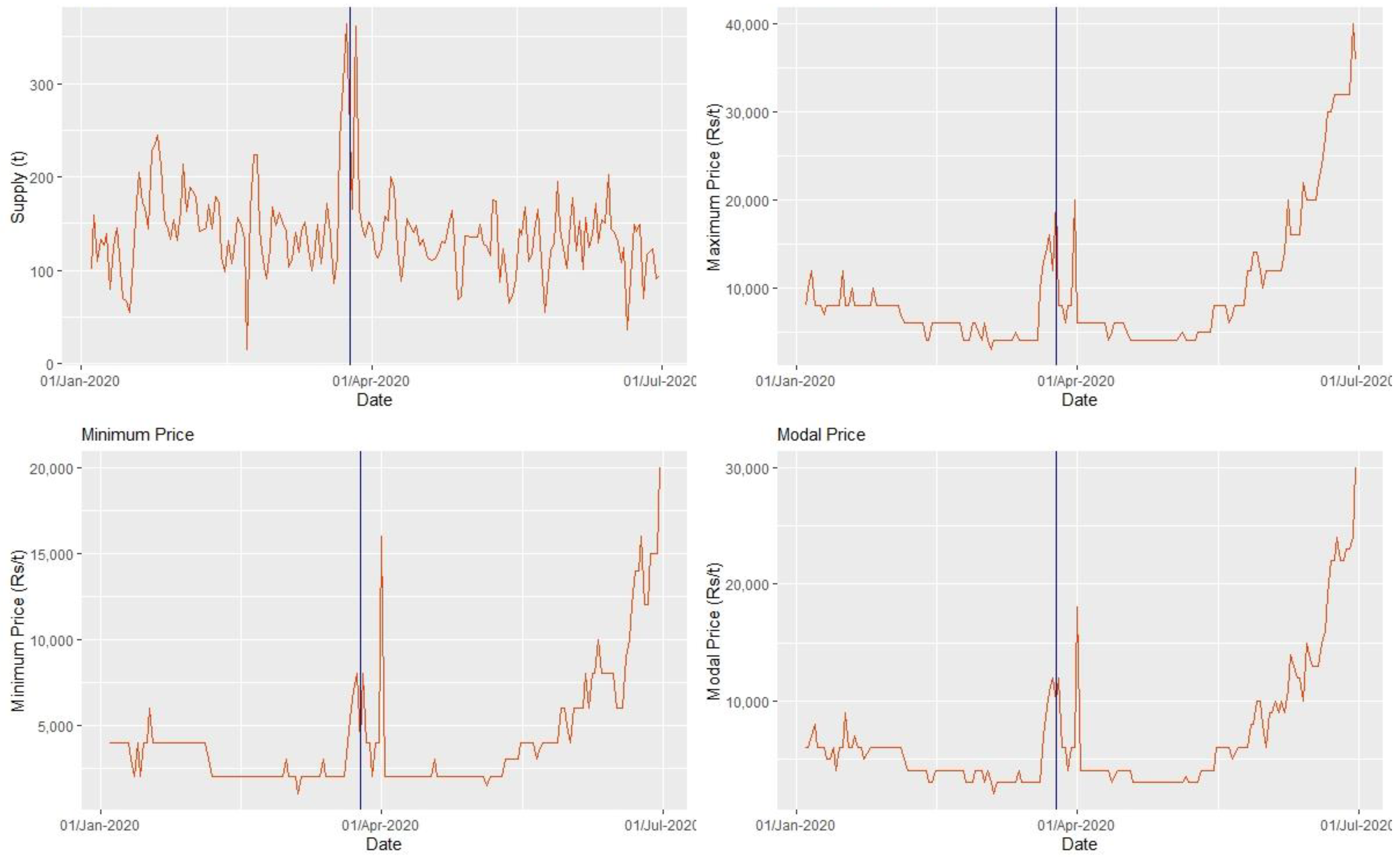
2.1. Data Description

The secondary data on tomato prices and arrivals were collected daily from 1 January 2020 to 30 June 2020 from the website http://tsmarketing.in/DailyArrivalsnPricesCommBetweenDates.aspx, accessed on 12 September 2020. The Government of India announced a nationwide lockdown from 25 March 2021 to 30 June 2020; thus, 25 March 2020 was considered as the intervention date and the data from 1 January 2020 to 24 March 2020 were considered as the pre-intervention period, whereas the data from 25 March 2021 to 30 June 2020 were considered as the post-intervention period. For modeling and forecasting, the data from 1 January 2020 to 23 June 2020 was used for model building and the data from 24 June 2020 to 30 June 2020 were used for model testing and validation. The map of the study area is shown in the Figure 1.

2.2. ARIMA Model

The Box–Jenkins [2] ARIMA is the most commonly used model in forecasting time series data. When the time series Yt is non-stationary or integrated, this procedure is an amalgamation of the ARMA process. To build the ARMA model in the case, the series must be differenced to make it stationary, and this differenced series, which is now stationary, must be subjected to ARIMA model fitting. This procedure is known as ARIMA (p,d,q), where p and q denote the number of AR and MA terms, respectively, and d denotes the order of differencing required to make the series stationary. An ARIMA model is expressed by the following expression:

Ø(B)(1 − B)^dY_t = θ(B)ε_t…

(1)

where:

Ø(B) = 1 − Ø₁B¹ − Ø₂B² − … − Øp B^P (autoregressive parameter)

Ø(B) = 1 − Ø₁B¹ − Ø₂B² − … − Øp B^q (Moving average parameter)

where d = differencing term, B = backshift operator, i.e., B^aY_t = Y_t−aε_t = white noise or error term. The ARIMA methodology is conducted in three steps, namely identification, estimation and diagnostic checking. For diagnostic checking, the Box–Pierce non-correlation test is most commonly used.

2.3. ARIMA Intervention Model

ARIMA intervention analysis [10] is a time series analysis technique that uses modelling approaches to incorporate the effect of exogenous forces or interventions. Government policies, strikes, earthquakes, price shifts, folds, pandemic, and other unforeseen catastrophes are all examples of interventions. It produces unexpected shifts in time series. Simply put, intervention analysis in time series refers to the study of how a series mean level changes as a result of an intervention.

$$Y_t=\frac{\omega \left(B\right)}{\delta \left(B\right)}{B}^b{I}_t+\frac{\theta \left(B\right)}{\varphi \left(B\right)}{\epsilon }_t$$

(2)

In this, the dependent variable is Y_t, indicator variable. I_t = indicator variable coded according to the type of intervention (step, pulse/point, and impulse). Here, δ(B) = 1 + δ₁ B + … δ_r B^r is the slope parameter, ω(B) = ω₀ + ω₁ B + … ω_s B^s is the impact parameter, φ(B) = 1 − φ₁ B − φ₂B² − … − φ_p B^p is the autoregressive parameter, θ(B) = 1 − θ₁ B − θ₂B² − … − θ_qB^q is the moving average parameter, b is the delay parameter, B is the backshift operator, i.e., B^aY_t = Y_t−a, ε_t is the white noise or error term. The step intervention occurs at a specific point in time and persist over successive time periods. The impact of the step intervention may be stable over time, or it may rise or diminish.

The indicator variable is coded as follows since the occurrence of COVID-19 is a step intervention type, I_t = 0, t < T′ and 1, t ≥ T′. The COVID-19 intervention, which was classified as a lockdown, began on March 25 2020 and was later extended in multiple phases. As a result, the indicator variable I_twas given a value of 0 before intervention period and 1 during the intervention period.

2.4. Support Vector Regression (SVR) Model

The SVR model was basically developed for classification problem, later adopted to regression problem by adding ε-insensitive loss function [32]. The main concept behind SVR is to solve a nonlinear regression in a linear manner by transferring nonlinear input data from a lower dimensional feature space to a higher dimensional feature space. The SVR estimation function is written as follows:

$$f\left(x\right)={\theta }^T\Phi \left(X\right)+b$$

(3)

where Φ(.) stands for a nonlinear space transformation, is the weight vector, and b stands for the bias. By further introducing a kernel function, θ is no longer needed to be given explicitly in the SVR estimation function, which becomes:

$$f\left(x\right)={\displaystyle \sum }_{i=1}^n\left(a_i-a_i{}^{*}\right)k\left(x,x_i\right)+b$$

(4)

where $k\left(x,x_i\right)=\Phi {\left(x_i\right)}^T\Phi \left(x_i\right)$ is the kernel function. The radial basis function (RBF) kernel function is the most commonly used kernel function in SVR and is represented as follows:

$$\left(x,x_i\right)=\exp \left(-\gamma \Vert x-x_i\Vert {}^2\right)$$

(5)

The coefficients W and b are estimated from data by minimizing the following regularized risk function:

$$R\left(\theta \right)=\frac{1}{2}{\Vert w\Vert }^2+C\left[\frac{1}{N}{\displaystyle \sum }_{i=1}^N{L}_{\epsilon }\left(y_i,f\left(x_i\right)\right)\right]$$

(6)

This regularized risk function minimizes both the empirical error and regularized term simultaneously, which helps in avoiding both under- and overfitting of the model. In Equation (6), the first term $\frac{1}{2}{\Vert w\Vert }^2$ is called the ‘regularized term’, which measures the flatness of the function. Minimizing $\frac{1}{2}{\Vert w\Vert }^2$ will make a function as flat as possible. The second term $\frac{1}{N}{{\displaystyle \sum }}_{i=1}^N{L}_{\epsilon }\left(y_i,f\left(x_i\right)\right)$ is called ‘empirical error’, which was estimated by the Vapnik ε-insensitive loss function as follows:

$$L_{\epsilon }\left(y_i,f\left(x_i\right)\right)=f\left(x\right)=\{\begin{array}{c}\left|y_i,f\left(x_i\right)-\epsilon \right|; \left|y_i-f\left(x_i\right)\right|\ge \epsilon ,\\ 0 \left|y_i-f\left(x_i\right)\right|<\epsilon , \end{array}$$

(7)

The performance of the RBF kernel function requires the optimization of two hyper-parameters: regularization parameter C, which balances the complexity and approximation accuracy of the model; and Kernel bandwidth parameter γ, which represents the variance of the RBF kernel function [33].

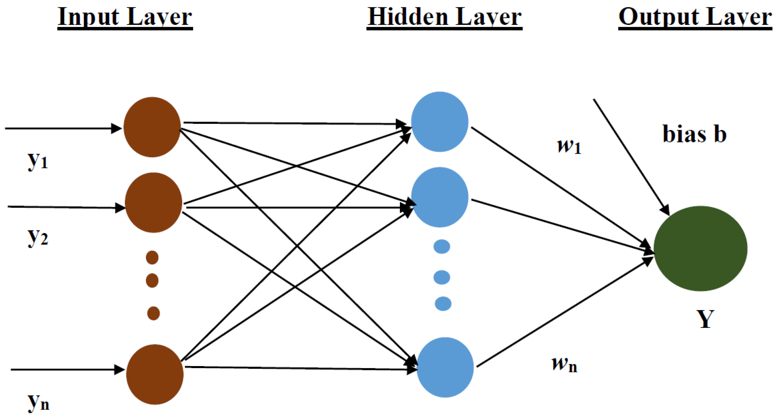
2.5. Artificial Neural Network (ANN) Model

The ANN is the most widely used AI technique in the last three decades in time series modelling and prediction. In the field of time series modelling, ANN is commonly referred to as an autoregressive neural network because it considers time lags as inputs. The time series framework for ANN can be mathematically modelled using a neural network with implicit functional representation of time. The general expression for the final output Y of a multilayer autoregressive neural network with feedforward is expressed as follows:

$$Y_t={\alpha }_0+{\displaystyle \sum }_{j=1}^q{\alpha }_{j}g\left({\beta }_{0j}+{\displaystyle \sum }_{i=1}^p{\beta }_{ij}{Y}_{t-p}\right)+{\epsilon }_t$$

(8)

where ${\alpha }_j\left(j=0,1,2,\dots ,q\right)$ and ${\beta }_{ij}\left(i=0,1,2,\dots ,p, j=0,1,2,\dots ,q\right)$ are the model parameters, also called the synopsis weights; p is the number of input nodes; q is the number of hidden nodes; and $g$ is the activation function. The training part in ANN minimizes the error function between actual and predicted values. The error function of autoregressive ANN is expressed as follows:

$$E=\frac{1}{N}{\displaystyle \sum }_{t=1}^N{(e_t)}^2=\frac{1}{N}{\displaystyle \sum }_{t=1}^N{\left\{X_t-(w_0+({\displaystyle \sum }_{J=1}^Q{w}_{J}g\left(w_{oj}+{\displaystyle \sum }_{i=1}^P{w}_{ij}{X}_{t-i}))\right)\right\}}^2$$

(9)

where N is the total number of error terms. The parameters of the neural network $w_{ij}$ are changed by a number of changes in $\Delta w_{ij}$ as $\Delta w_{ij}=-\eta \frac{\partial E}{\partial w_{ij}}$, where $\eta$ is the learning rate [34]. The schematic representation of neural network structure is depicted in Figure 2.

2.6. Artificial Intelligence (AI)-Based Intervention Models

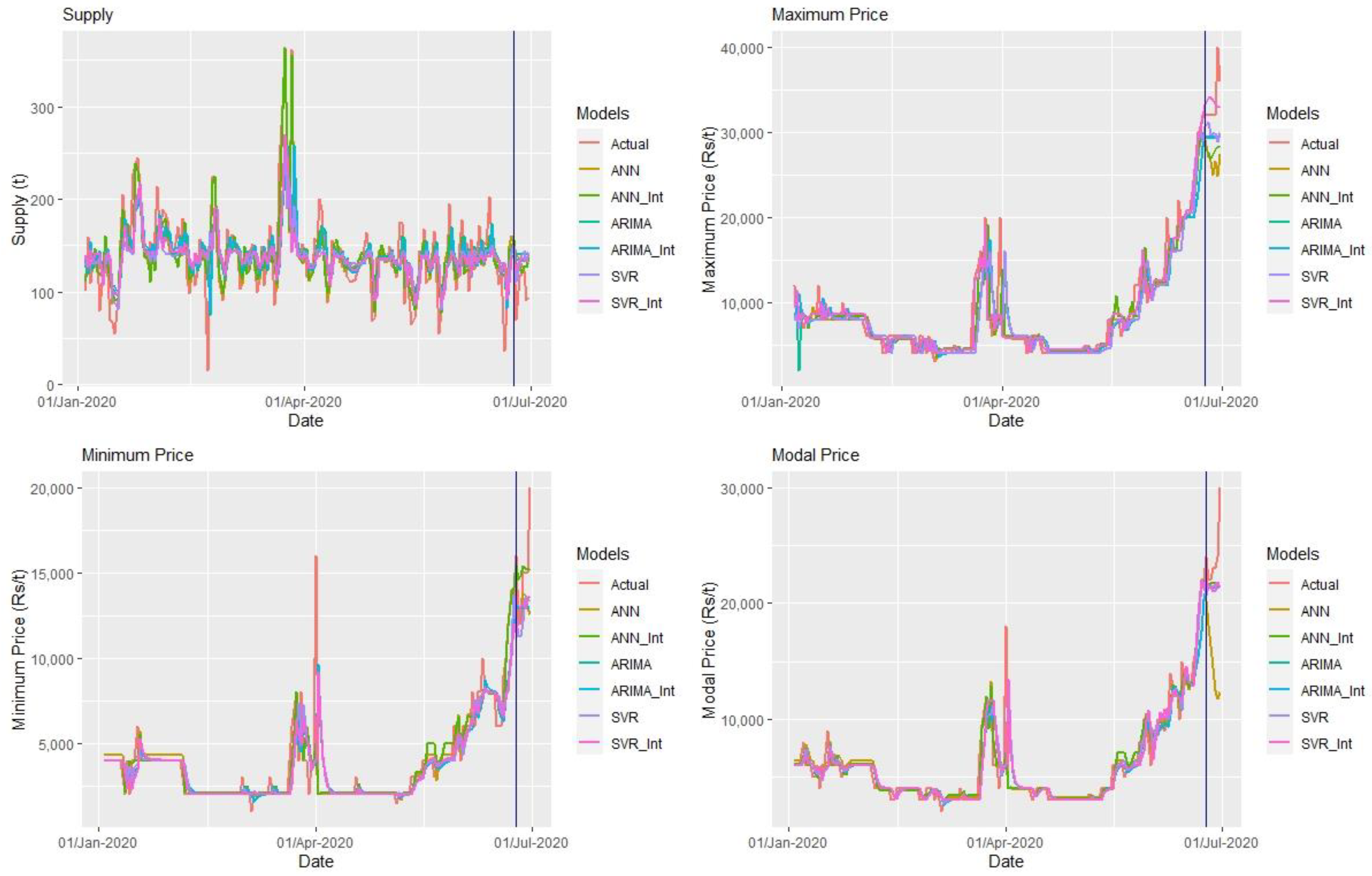
The traditional artificial intelligence approach allows for forecasting based solely on the past values of the forecast variables. The model assumes that the future values of a variable are determined by its previous values as a well as the values of exogenous variable in the past. The artificial intelligence intervention model is a modified version of the artificial intelligence model that adds an additional independent variable called the intervention variables; this model is also referred to as the vector artificial intelligence model. The artificial intelligence forecasting models typically assume that each observed value is an unknown nonlinear function F of clagst₁, t₂, …, t_c, for a given univariate time series {x_t, t = 1, 2, …, n}, where x_tϵ R,

$$x_t=F\left(x_{t-t1}, x_{t-t2}, \dots , x_{t-tc}\right)+{\epsilon }_t$$

(10)

where the error ε_t is error of zero mean. Next, we assume that m interventions have been observed throughout time periods r₁, r₂, …, r_m. Depending on the nature of the interventions, we define m auxiliary variables δ₁^t, δ₂^t,…, δ_m^t. As a result, we can have a nonlinear forecasting model with clagst₁, t₂, …, t_c and m interventions:

$$x_t=F\left(x_{t-t1}, x_{t-t2}, \dots , x_{t-tc} , {\delta }_1{}^t, {\delta }_2{}^t, \dots , {\delta }_m{}^t\right)+{\epsilon }_t$$

(11)

In this article, two AI-based intervention models, namely SVR and ANN intervention models, were developed by the intervention concept explained in this section. Along with the above explained models, the BDS (Brock–Dechert–Scheinman) test for non-linearity checking and the Diebold–Mariano test for significance comparison of model performance are used in this study; details about these tests are available in the literature [35,36]. Finally, the mean absolute percentage error (MAPE) is the most commonly used measure for forecasting error.

$$MAPE=\frac{1}{N}\left|\frac{A-F}{A}\right|\times 100$$

(12)

where A is the actual value, F is forecast or predicted value, and N is the number of observations.

3. Results

Figure 3 shows the time series of supplies, maximum price, minimum price, and modal price in the Gudimalkapur market, where the blue line indicates the intervention date, i.e., 25 March 2020, when the government of India announced the lockdown.

Table 1. Descriptive statistics of Gudimalakpur market.

Statistic	Supply (t)	Maximum Price (Rs/t)	Minimum Price (Rs/t)	Modal Price (Rs/t)
Observation	179	179	179	179
Mean	139.74	9346.37	4127.78	6612.60
Median	137.4	6000	3000	4500
Mode	164.2	4000	2000	4000
Standard Deviation	46.42	7335.47	3310.34	5079.42
Minimum	15.15	3000	1000	2000
Maximum	363.8	40,000	20,000	30,000
Skewness	1.47	2.15	2.33	2.24
Kurtosis	5.84	4.32	5.75	5.07
Coefficient of Variation (%)	31.22	78.48	80.20	76.81

shows the descriptive statistics for all four series of the Gudimalkapur market. The arrival price series are highly skewed and leptokurtic. The coefficient of variation for all four series are 31%, 78%, 80%, and 76% for arrivals, maximum price, minimum price, and modal price, respectively, indicating that the data are inherently heterogeneous.

The BDS (Brock–Dechert–Scheinman) test indicates that the data under consideration is nonlinear as the probability value p 0.0001 for all the four series of Gudimalkapur market is given in

Table 2. BDS test for non-linearity.

Time Series	Eps (1)		Eps (2)		Eps (3)		Eps (4)
	Statistic at m = 2	Statistic at m = 3	Statistic at m = 2	Statistic at m = 3	Statistic at m = 2	Statistic at m = 3	Statistic at m = 2	Statistic at m = 3
Supply	4.19 (p < 0.001)	4.65 (p < 0.001)	5.44 (p < 0.001)	5.55 (p < 0.001)	6.69 (p < 0.001)	6.92 (p < 0.001)	7.48 (p < 0.001)	7.83 (p < 0.001)
Maximum Price	20.47 (p < 0.001)	25.81 (p < 0.001)	16.13 (p < 0.001)	16.86 (p < 0.001)	14.58 (p < 0.001)	14.36 (p < 0.001)	16.15 (p < 0.001)	15.27 (p < 0.001)
Minimum Price	27.02 (p < 0.001)	39.03 (p < 0.001)	15.07 (p < 0.001)	15.86 (p < 0.001)	13.53 (p < 0.001)	13.66 (p < 0.001)	12.38 (p < 0.001)	11.55 (p < 0.001)
Modal Price	20.51 (p < 0.0001)	25.15 (p < 0.001)	16.31 (p < 0.001)	17.07 (p < 0.001)	14.35 (p < 0.001)	14.55 (p < 0.001)	13.48 (p < 0.001)	12.55 (p < 0.001)

.

3.1. Results of ARIMA Models

For the series of supplies in Gudimalkapur market, ARIMA (1,0,0) was found to be suitable; for the series of prices, ARIMA (0,1,1), ARIMA (0,1,1), ARIMA (0,1,1) were found suitable for maximum price, minimum price, and modal price, respectively (

Table 3. Parameter Estimation of ARIMA Model.

Time Series	Model	Parameters	Estimation	S. E	Z Value	p Value	Model Fitting		Box–Pierce Non-Correlation Test
									Original	Residuals
Supply	ARIMA (1,0,0)	AR1	0.53	0.06	8.33	<0.001	Log-likelihood	−1292.85	X-squared = 51.378 (p = 0.0001)	X-squared = 0.152 (p = 0.61)
							AIC	2591.7
							BIC	2601.19
Maximum Price	ARIMA (0,1,1)	MA1	−0.37	0.072	−5.059	<0.001	Log-likelihood	−1180.29	X-squared = 144.61 (p = 0.0001)	X-squared = 0.06 (p = 0.81)
							AIC	2364.58
							BIC	2370.9
Minimum Price	ARIMA (0,1,1)	MA1	−0.54	0.07	−7.24	<0.001	Log-likelihood	−1117.4	X-squared = 115.34 (p = 0.0001)	X-squared = 0.001 (p = 0.97)
							AIC	2238.8
							BIC	2245.12
Modal Price	ARIMA (0,1,1)	MA1	−0.38	0.07	−4.90	<0.001	Log-likelihood	−1140.81	X-squared = 138.85 (p = 0.0001)	X-squared = 0.0003 (p = 0.98)
							AIC	2285.62
							BIC	2291.93

). The parameters of the models were estimated using the maximum likelihood method and the estimated values are given in Table 3. Diagnostic testing of the residuals was performed using the Box–Pierce non-correlation test for residuals and the results show that the residuals are not autocorrelated and random as the probability values of significance are 0.61, 0.81, 0.97, and 0.98 for the arrivals, maximum price, minimum price, and modal price, respectively.

3.2. Results ARIMA Intervention Models

Like the ARIMA model, the ARIMA intervention models were built for all four time series dates. The ARIMA intervention model (1,0,0) was found to be appropriate for supply series, and the ARIMA intervention models (0,0,1), ARIMA intervention models (0,0,1), and ARIMA intervention models (0,0,1) were found to be appropriate for the maximum price, minimum price, and modal price, respectively. The parameters estimated using maximum likelihood estimation techniques are shown in

Table 4. Parameter estimation of ARIMA intervention model.

Time Series	Model	Parameters	Estimation	S. E	Z Value	p Value	Model Fitting		Box–Pierce Non- Correlation Test
									Original	Residuals
Supply	ARIMA (1,0,0)	AR1	0.53	0.06	8.25	<0.001	Log-likelihood	−1292.74	X-squared = 51.37 (p = 0.0001)	X-squared = 0.13 (p = 0.71)
		Impact $\left(\omega \right)$	−5.73	2.86	−2.00	0.023	AIC	2593.49
							BIC	2606.15
Maximum Price	ARIMA (0,1,1)	MA1	−0.36	0.07	−4.86	<0.001	Log-likelihood	−1179.93	X-squared = 144.61 (p = 0.0001)	X-squared = 0.04 (p = 0.83)
		Impact $\left(\omega \right)$	171.29	90.10	1.90	0.39	AIC	2365.85
							BIC	2375.33
Minimum Price	ARIMA (0,1,1)	MA1	−0.52	0.07	−6.91	<0.001	Log-likelihood	−1116.43	X-squared = 115.34 (p = 0.0001)	X-squared = 0.007 (p = 0.93)
		Impact $\left(\omega \right)$	179.82	84.82	2.12	0.017	AIC	2238.86
							BIC	2248.34
Modal Price	ARIMA (0,1,1)	MA1	−0.38	0.07	−4.88	<0.001	Log-likelihood	−1140.49	X-squared = 138.85 (p = 0.0001)	X-squared = 0.0005 (p = 0.98)
		Impact $\left(\omega \right)$	124.88	70.91	1.76	0.039	AIC	2286.99
							BIC	2296.46

. The intervention parameters (impact (ω)) are estimated as −5.73 (p = 0.023), 171.29 (p = 0.029), 179.82 (p = 0.017), and 124. 88 (p = 0.039) for supplies, maximum price, minimum price, and modal price, respectively. The results show that the lockdown had a negative impact on tomato supplies and a positive impact on price series, which means about 600 kg of tomato per day less supplies. The results showed that there was an increase in the maximum price by Rs.17.1/t/day, minimum price by Rs.18/t/day, and average price by Rs.12.5/t/day for Gudimalkapur market. The fitted models were appropriate as the Box–Pierce non-correlation test for the residuals is not autocorrelated and random as the probability values of significance are 0.71, 0.83, 0.93, and 0.98 for arrivals, maximum price, minimum price, and modal price, respectively. Similar results were obtained in the study conducted by Ray and others [12] on cotton yield prediction. It was found that the performance of ARIMA intervention models was superior to conventional ARIMA models for all the three locations.

3.3. Results of SVR and SVR Intervention Models

Based on the required user-defined parameters, the SVR model and SVR intervention models (

Table 5. Parameter specification of SVR and SVR intervention model.

Parameter	Supply		Maximum Price		Minimum Price		Modal Price
	SVR	SVR Intervention	SVR	SVR Intervention	SVR	SVR Intervention	SVR	SVR Intervention
Kernel Function	Radial
No. of S.Vs	117	111	118	115	123	133	116	112
Cost	2.1	2.29	2.4	2.1	2	2	1.94	2.07
Gamma	1	0.5	1	0.5	1	0.5	1	0.5
Epsilon	0.01	0.001	0.0001	0.0001	0.001	0.001	0.0001	0.0001
Box–pierce non-correlation test	0.364	0.03	0.05	0.005	0.30	0.14		0.07
p-value	0.827	0.721	0.963	0.654	0.782	0.985	0.924	0.754

) were constructed. The radial basis function (RBF) is used as the kernel function. The number of support vectors obtained at optimal level was 117 for arrival series and 118, 123, 116 for maximum price, minimum price, and modal price, respectively. For the support vector regression with intervention model, the number of support vectors obtained at the optimal level was 111 for the arrival series and 115, 133, and 112 for the maximum price, minimum price, and maximum price, respectively. The Box–Pierce non-autocorrelation shows that the residuals are not autocorrelated or random (Table 5).

3.4. Results of ANN and ANN Intervention Model

Given the low training MAPE, appropriate models were selected with three tapped and ten hidden nodes (3: 10S: 1L) for the arrival series and maximum price, respectively, and two tapped and nine nodes (2: 9S: 1L) and two tapped and nine hidden nodes (2: 9S:1L) for the minimum price and modal price, respectively. Diagnostic testing of the residuals by the Box–Pierce test is performed after model fitting. The residuals were not autocorrelated or random as the probability values are 0.79, 0.69, 0.63, and 0.73 for the arrivals, maximum price, minimum price, and modal price, respectively. For the arrival and maximum price series of the Gudimalkapur market, the intervention model with three tapped nodes and ten hidden nodes and one exogenous intervention variable (4: 10S: 1L) was selected; and for the minimum price and modal price, the model with (3;9S: 2L) and (3:9S: 1L), respectively, was selected due to low MAPE values. The sigmoidal activation function was used in the input to the hidden layer and the linear activation function from the hidden to output layer. The residual values of all four series of the Gudimalkapur market are shown in

Table 6. Parameter specification of ANN and ANN intervention model.

Parameter	Arrivals		Maximum Price		Minimum Price		Modal Price
	ANN	ANN Intervention	ANN	ANN Intervention	ANN	ANN Intervention	ANN	ANN Intervention
Input Lag	3	3	3	3	2	2	2	2
Dependent/Output Variable	1	1	1	1	1	1	1	1
Hidden Layers	1	1	1	1	1	1	1	1
Hidden Nodes	10	10	10	10	9	9	9	9
Exogenous Variables	1	7	1	7	1	7	1	7
Model	3:10S:1L	4:10S:1L	3:10S:1L	4:10S:1L	2:9S:1L	3:9S:1L	2:9S:1L	3:9S:1L
Total Number of Parameters	51	61	51	61	37	46	37	46
Network Type	Feed Forward
Activation Function I:H	Sigmoidal
Activation Function H:O	Identity
Box–Pierce Non-Correlation Test for Residuals	0.06 (p = 0.79)	0.003 (p = 0.95)	0.16 (p = 0.69)	0.04 (p = 0.83)	0.22 (p = 0.63)	0.60 (p = 0.43)	0.11 (p = 0.73)	0.19 (p = 0.66)

, indicating that the residuals are not autocorrelated or random in nature.

4. Discussion

The results show that the lockdown has a negative effect on tomato supply and a positive effect on tomato price series. About 600 kg of tomatoes per day were supplied less due to the lockdown. The results also showed that the maximum price increased by Rs.17.1/t/day, minimum price increased by Rs.18/t/day, and modal price increased by Rs.12.5/t/day. The negative impact of the lockdown on deliveries is likely to be related to the decline in production during this period and could also be due to the problems faced by farmers and suppliers in transporting tomatoes to the market. The low volume of deliveries might have contributed to the higher price, which is evident from the positive impact of the lockdown on the price series. The forecasting performance of the six selected models—ARIMA, ARIMA intervention, SVR, SVR intervention, ANN, and ANN intervention—was evaluated for their forecasting ability based on model errors in both training and test data sets. Based on the MAPE values obtained (

Table 7. Comparison of model performance in terms of MAPE in training sets.

Time Series	ARIMA		ARIMA Intervention		SVR		SVR Intervention		ANN		ANN Intervention
	Training	Testing	Training	Testing	Training	Testing	Training	Testing	Training	Testing	Training	Testing
Supply	25.52	37.86	25.20	31.81	23.98	33.12	24.16	29.02	18.4	29.86	16.52	27.84
Maximum Price	12.40	10.77	12.28	10.68	11.13	10.09	11.01	10.02	9.78	8.98	8.95	6.51
Minimum Price	17.24	16.04	16.78	15.78	16.24	15.35	15.87	15.04	12.03	13.28	11.16	11.18
Modal Price	13.04	10.14	12.96	10.04	12.81	9.78	12.35	9.67	10.77	9.76	9.83	8.52

), the ANN intervention model outperformed the ANN and other models in both model building and validation data sets for the supply and price time series. The ANN intervention model also performed better than ANN and the other models in both the training and test data sets for the price series. The predicted values of the ARIMA and ARIMA intervention models, as well as the SVR models, produced the same predicted values for all days, implying that the model does not have the generalization ability to provide different predicted values compared to the ANN intervention models.

In this study, the developed AI models outperformed the classic ARIMA and ARIMA intervention models. Among the AI models, the ANN intervention model performed better than all other models in both training and test data sets. The performance hierarchy of the Gudimalkapur market in the training and testing datasets is ANN intervention ANN SVR intervention SVR ARIMA intervention ARIMA in all four datasets. The MAPE values only show the observed difference between the actual and predicted values. To overcome this, we used DM test statistics to identify the significance difference in performance between the different evolutions. The DM test shows that the ANN intervention model was significantly superior to the other models in both the training and test data sets, and their intercombinational superiority is shown in

Table 8. Diebold–Mariano test for significance comparison of different models in training and testing data sets.

Time Series	Data Type	M1, M2	M1, M3	M1, M4	M1, M5	M1, M6	M2, M3	M2, M4	M2, M5	M2, M6	M3, M4	M3, M5	M3, M6	M4, M5	M5, M6
Supply	Training	2.42 (0.016)	0.73 (0.466)	2.70 (0.007)	1.77 (0.076)	1.79 (0.075)	−2.31 (0.021)	2.81 (0.003)	−2.78 (0.006)	−2.72 (0.007)	2.60 (0.009)	1.70 (0.090)	1.82 (0.070)	−3.09 (0.002)	0.33 (0.740)
	Testing	2.79 (0.031)	3.36 (0.015)	3.65 (0.01)	1.28 (0.241)	1.84 (0.107)	2.36 (0.556)	−2.17 (0.073)	0.47 (0.648)	0.55 (0.597)	−3.20 (0.019)	0.47 (0.649)	0.61 (0.055)	0.19 (0.855)	−0.30 (0.767)
Maximum price	Training	2.74 (0.006)	0.27 (0.788)	2.82 (0.005)	1.78 (0.075)	4.15 (<0.001)	−2.68 (0.008)	0.41 (0.683)	−1.07 (0.285)	2.66 (0.008)	2.77 (0.006)	1.62 (0.106)	4.08 (<0.001)	−0.98 (0.323)	3.70 (0.0002)
	Testing	−7.10 (0.0004)	3.27 (0.017)	−4.10 (0.006)	1.24 (0.254)	2.09 (0.074)	7.08 (0.0004)	7.09 (0.0003)	2.71 (0.030)	2.25 (0.058)	−4.11 (0.006)	1.08 (0.314)	2.07 (0.076)	4.48 (0.002)	1.49 (0.177)
Minimum price	Training	2.38 (0.015)	0.43 (0.667)	2.41 (0.017)	0.44 (0.659)	1.07 (0.284)	−2.18 (0.03)	0.76 (0.448)	−2.73 (0.006)	−2.53 (0.012)	2.23 (0.027)	0.13 (0.899)	0.66 (0.509)	−2.71 (0.007)	0.31 (0.759)
	Testing	2.32 (0.06)	2.02 (0.089)	1.19 (0.28)	0.81 (0.442)	0.32 (0.757)	−0.03 (0.977)	1.03 (0.339)	0.03 (0.973)	−0.11 (0.918)	1.13 (0.30)	0.41 (0.690)	0.06 (0.948)	−1.21 (0.265)	−0.24 (0.816)
Modal price	Training	2.34 (0.02)	0.06 (0.54)	2.31 (0.018)	1.53 (0.128)	1.60 (0.111)	−2.31 (0.022)	0.45 (0.651)	1.47 (0.143)	1.51 (0.130)	2.35 (0.02)	−2.17 (0.031)	−2.09 (0.037)	−2.33 (0.025)	0.27 (0.787)
	Testing	−4.83 (0.003)	2.52 (0.045)	−3.20 (0.018)	1.06 (0.324)	1.11 (0.301)	4.83 (0.003)	4.81 (0.003)	1.01 (0.346)	1.01 (0.346)	−3.19 (0.018)	2.57 (0.037)	2.63 (0.033)	−1.69 (0.135)	−0.22 (0.830)

. The actual vs. fitted plots of the different models for all four markets are shown in Figure 4 and the actual vs. fitted values are given in supplementary Tables S1 and S2.

The empirical results show the superiority of the ANN intervention model over the other models examined in this study. The superiority of the ANN intervention model may be due to its ability to mimic the nonlinear and detailed nature of the data while allowing for an external intervention variable, making it very useful in explaining the dynamics of the impact of the COVID-19 pandemic on tomato supply and price fluctuations in the market.

Similar results were obtained in the study conducted by Ray and others [12], who found a positive impact of Bacillus thuringiensis technology on the cotton yield. Another study reported that the decline in Chinese manufacturing during the reported period had a negative impact on stock market prices, as revealed by the ARIMA intervention model results [14]. A study conducted by Ismail and others [37] also reported similar results; they found a negative impact of bombing on the tourism industry using ARIMA intervention model. Several studies [38,39,40,41] revealed that artificial-intelligence-based models, namely ANN and SVR, outperformed the classical ARIMA models in predicting the time series data in agriculture and other fields. Harini and others [24] also showed that ANN-based intervention models performed better compared to classical models in clinical intervention prediction.

5. Conclusions

The present study was undertaken to investigate the impact of the COVID-19 lockdown on the supplies and prices of tomato in Hyderabad market in Telangana state, India. The ARIMA intervention model significantly confirmed that there was a negative impact on the supply, but a positive impact on the price of tomato in examined market. The spillover effects from the pandemic to the tomato supplies have been significant with the increase in transportation costs, which resulted in an increase in the prices of the tomato and might also have contributed to low consumption levels. Additionally, the high prices of tomato combined with low supplies might have contributed to the increased vulnerability of the producers and food insecurity of the consumers. The classical times series models such as ARIMA and ARIMA intervention models were used in analyzing the impact of policies or sudden changes in agricultural impact studies. These models fail to capture the nonlinear structure present in data sets. To overcome this problem, we have developed ANN- and SVR-based intervention models by incorporating the intervention variable as an exogenous variable in the input layer. The data considered were nonlinear in nature, the classical linear time series models, namely the ARIMA and ARIMA intervention time series models, were not able to capture the nonlinear and chaotic patterns in the data identified by the BDS test. Therefore, an AI-based model was applied in this study to capture the nonlinear and complex nature of the data. The ANN intervention model outperformed all other models for modeling and predicting supply and price series of tomato; thus, it can be used to study the nonlinear complex nature of data under intervention in other time series data. The AI-based intervention models developed in this study can be used to evaluate the potential effects of government policies and programmes. The model has a wider scope to study the impact of interventions in agriculture. For example, it can be applied to study the impact of government subsidies on inputs in agriculture, price support to the producers, and the impact of pest and disease outbreak, to forecast the supply and price of agricultural products.

References

1. National Horticultual Boad; Ministry of Agriculture and Farmers Welfare; Governament of India. Horticultural Statistics at a Glance. 2018. Available online: http://nhb.gov.in/statistics/Publication/Horticulture%20Statistics%20at%20a%20Glance-2018.pdf (accessed on 12 September 2020).
2. Box, G.; Jenkins, G. Time Series Analysis: Forecasting and Control; Holden-Day: San Francisco, CA, USA, 1970. [Google Scholar]
3. Naveena, K.; Rathod, S.; Shukla, G.; Yogish, K.J. Forecasting of coconut production in India: Suitable time series models. Int. J. Agric. Eng. 2014, 7, 190–193. [Google Scholar]
4. Jalikatti, V.N.; Raghavendra, C.; Ahmad, D.G.; Shreya, A.; Sheikh, S. Forecasting the prices of onion in belgaum market of northern Karnataka using ARIMA technique. Int. J. Agric. Econ. 2014, 5, 153–159. [Google Scholar] [CrossRef]
5. Jeong, M.; Lee, Y.J.; Choe, Y. Forecasting agricultural commodity price: The case of onion. J. Res. Humanit. Soc. Sci. 2017, 5, 78–81. [Google Scholar]
6. Kaur, L.; Dhaliwal, T.; Rangi, P.S.; Singh, N. An economic analysis of tomato arrivals and prices in Punjab. Indian J. Agril. Mktg. 2005, 19, 61–67. [Google Scholar]
7. Rathod, S.; Singh, K.N.; Arya, P.; Ray, M.; Mukherjee, A.; Sinha, K.; Kumar, P.; Shekhawat, R.S. Forecasting maize yield using ARIMA-Genetic Algorithm approach. J. Outlook Agr. 2017, 46, 265–271. [Google Scholar] [CrossRef]
8. Rathod, S.; Singh, K.N.; Patil, S.G.; Naik, R.H.; Ray, M.; Meena, V.S. Modelling and forecasting of oilseed production of India through artificial intelligence techniques. Indian J. Agric. Sci. 2018, 88, 22–27. [Google Scholar]
9. Tatarintsev, M.; Korchagin, S.; Nikitin, P.; Gorokhova, R.; Bystrenina, I.; Serdechnyy, D. Analysis of the Forecast Price as a Factor of Sustainable Development of Agriculture. Agronomy 2021, 11, 1235. [Google Scholar] [CrossRef]
10. Box, G.E.P.; Tiao, G.C. Intervention analysis with application to Economic and Environmental Problems. J. Am. Stat. Assoc. 1995, 70, 70–79. [Google Scholar] [CrossRef]
11. Bianchi, L.; Jeffrey, J.; Choudary, H.R. Improving forecasting for telemarketing centres by ARIMA modelling with intervention. Int. J. Forecast. 1998, 14, 497–504. [Google Scholar] [CrossRef] [Green Version]
12. Ray, M.; Ramasubramanian, V.; Anil, R. Applications of time series intervention modelling for modelling and forecasting cotton yield. Stat. Appl. 2014, 12, 61–70. [Google Scholar]
13. Ramasubramanian, V.; Ray, M. Power computation-based performance assessment of ARIMA intervention modelling. J. Indian Soc. Agric. Stat. 2019, 73, 233–242. [Google Scholar]
14. Jeffrey, E.J.; Kyner, E. ARIMA modelling with intervention to forecast and analyse Chinese stock prices. Int. J. Agric. Mark. 2011, 3, 53–58. [Google Scholar] [CrossRef]
15. Corchuelo Martínez-Azúa, B.; López-Salazar, P.E.; Sama-Berrocal, C. Impact of the COVID-19 Pandemic on Agri-Food Companies in the Region of Extremadura (Spain). Agronomy 2021, 11, 971. [Google Scholar] [CrossRef]
16. Di Marcantonio, F.; Twum, E.K.; Russo, C. Covid-19 Pandemic and Food Waste: An Empirical Analysis. Agronomy 2021, 11, 1063. [Google Scholar] [CrossRef]
17. Zhang, G.P.; Patuwo, E.; Hu, Y.M. Forecasting with Artificial Neural Networks: The State of the Art. Int. J. Forecast. 1998, 14, 35–62. [Google Scholar] [CrossRef]
18. Rathod, S.; Mishra, G.C. Statistical Models for Forecasting Mango and Banana Yield of Karnataka. India. J. Agric. Sci. Technol. 2018, 20, 803–816. Available online: https://jast.modares.ac.ir/article-23-19768-en.html (accessed on 10 September 2021).
19. Khan, T.; Sherazi, H.H.R.; Ali, M.; Letchmunan, S.; Butt, U.M. Deep Learning-Based Growth Prediction System: A Use Case of China Agriculture. Agronomy 2021, 11, 1551. [Google Scholar] [CrossRef]
20. Niazkar, H.R.; Niazkar, M. Application of artificial neural networks to predict the COVID-19 outbreak. Glob. Health Res. Policy 2020, 5, 50. [Google Scholar] [CrossRef]
21. Niazkar, M. Assessment of artificial intelligence models for calculating optimum properties of lined channels. J. Hydroinformatics 2020, 22, 1410–1423. [Google Scholar] [CrossRef]
22. Niazkar, M.; Talebbeydokthi, N.; Afzali, S.H. Bridge backwater estimation: A comparison between artificial intelligence models and explicit equations. Sci. Iran. 2020, 28, 573–585. [Google Scholar] [CrossRef]
23. Xun, Z.; Yu, L.; Wang, S. Assessing potentiality of support vector machine method in crude oil price forecasting. EURASIA J. Math. Sci. Technol. Educ. 2017, 13, 7893–7904. [Google Scholar] [CrossRef]
24. Harini, S.; Nathan, H.; Jhonson, A.; Anthony, L.C.; Peter, S.; Marzyeh, G. Clinical intervention prediction understanding with deep neural networks. In Proceedings of the 2nd Machine Learning for Healthcare Conference, PMLR, Boston, MA, USA, 19–20 August 2017; Volume 68, pp. 322–337. Available online: https://arxiv.org/abs/1705.08498v1 (accessed on 23 May 2017).
25. Hu, Z.; Ge, Q.; Shudi, L.; Boerwinkle, E.; Jin, L.; Xiong, M. Forecasting and Evaluating Multiple Interventions for COVID-19 Worldwide. Front. Artif. Intell. 2020, 3, 41. [Google Scholar] [CrossRef]
26. Jha, G.K.; Sinha, K. Agricultural Price Forecasting using Neural Network Model: An Innovative Information Delivery System. Agric. Econ. Res. Rev. 2013, 26, 229–239. [Google Scholar] [CrossRef] [Green Version]
27. Kuan, C.M.; White, H. Artificial Neural Networks: An Economic Perspective. Econom. Rev. 1994, 13, 1–91. [Google Scholar] [CrossRef]
28. Pai, P.F.; Lin, C.S. A Hybrid ARIMA and Support Vector Machines model in Stock Price Forecasting. Int. J. Manag. Sci. 2004, 33, 497–505. [Google Scholar] [CrossRef]
29. Shelke, R.D.; Kalyanker, S.C. Pattern of Market Arrivals of Tomato in Parbhani District of Maharashtra State. Int. J. Agric. Econ. 1998, 53, 423–425. [Google Scholar]
30. Bejo, K.S.; Mustaffha, S.; Ismail, I.W. Application of Artificial Neural Network in Predicting the Crop Yield: A Review. J. Food Sci. Eng. 2014, 4, 1–9. [Google Scholar]
31. Jhee, W.C.; Lee, K.C. A Neural Network Approach for the Identification of the Box-Jenkins Model. Comput. Neural Syst. 2009, 3, 323–339. [Google Scholar] [CrossRef]
32. Vapnik, V.N. The Nature of Statistical Learning Theory; Springer: New York, NY, USA, 1995. [Google Scholar] [CrossRef]
33. Smola, A.J.; Scholkopf, B.A. Tutorial on support vector regression, statistical computing. Stat. Comput. 2004, 14, 199–222. [Google Scholar] [CrossRef] [Green Version]
34. White, H. Learning in Artificial Neural Networks: A Statistical Perspective. Neural Comput. 1989, 1, 425–464. [Google Scholar] [CrossRef]
35. Brock, W.; Scheinkman, J.A.; Dechert, W.D.; LeBaron, B. A test for independence based on the correlation dimension. Econom. Rev. 1996, 15, 197–235. [Google Scholar] [CrossRef]
36. Diebold, F.X.; Mariano, R.S. Comparing predictive accuracy. J. Bus. Econ. Stats. 1995, 13, 253–263. Available online: http://www.jstor.org/stable/1392185 (accessed on 10 September 2021).
37. Ismail, Z.; Suhartono, S.; Yahaya, A.; Efend, R. Intervention Model for Analysing the Impact of Terrorism to Tourism Industry. J. Math. Stat. 2009, 5, 322–329. [Google Scholar]
38. Omolola, M.A.; Joel, O.B.; Abiodum, M.A.; Abubeker, H.; Christina, M.B.; Daniel, D.; Eyob, T. Application of Artificial Neural Network for Predicting Maize Production in South Africa. Agronomy 2019, 11, 1145. [Google Scholar] [CrossRef] [Green Version]
39. Rathod, S.; Mishra, G.; Singh, K.N. Hybrid time series models for forecasting banana production in Karnataka state, India. J. Indian Soc. Agric. Stat. 2017, 71, 193–200. [Google Scholar]
40. Kurumatani, K. Time Series Forecasting of Agricultural Product Prices Based on Recurrent Neural Networks and its Evaluation method. SN Appl. Sci. 2020, 2, 1434. [Google Scholar] [CrossRef]
41. Zhang, G.P. Time series forecasting using a hybrid ARIMA and neural network model. Neuro. Comput. 2003, 50, 159–175. [Google Scholar] [CrossRef]
Figure 1. Map of the study area.
Agronomy 11 01878 g001
Figure 2. Model structure of the artificial neural network.
Agronomy 11 01878 g002
Figure 3. Time series plots of the Gudimalkapur market.
Agronomy 11 01878 g003
Figure 4. Actual vs. fitted plots of tomato supply and prices for the Gudimalkapur market.
Agronomy 11 01878 g004