Does the Level of Financial Cognition Affect the Income of Rural Households? Based on the Moderating Effect of the Digital Financial Inclusion Index

Abstract

Financial cognitive ability is an important part of human capital, which has a direct impact on household income. The dual differences composed by rural residents’ cognition level and residents’ income make the relationship between the two complicated. Based on the analysis of the impact of financial cognitive level on rural household income, this paper takes into account the individual heterogeneity of financial cognition to build an unconditional quantile regression (UQR) model through the micro data of the China Household Financial Survey Project (CHFS). Incorporating the background of the rapid development of digital finance, this paper also studies the impact of rural residents’ financial cognition on household income. The empirical results of the article have the following conclusions: First, on the whole, the improvement of financial cognitive level promotes the increase of rural household income, but this promotion has significant differences at different quantile levels of household income. Second, the digital financial inclusion index in the region has a positive moderating effect on the impact of financial cognition on the income of rural households. Third, the heterogeneity of the impact of financial cognition on the income of rural households is reflected in the two aspects of regions and household assets.

1. Introduction

Financial cognitive ability is an important part of human capital [1], which has a direct impact on household income. With the rapid development of global finance in the 20th century [2,3], various financial institutions and products such as digital financial instruments [4] and green credit [5] have emerged one after another, which brings much volatility to the market [6]. Improving the level of financial cognition can enable people to receive financial information more effectively, identify fraud [7], consume rationally, and optimize the allocation of their own property [8], thereby increasing business income and property income, which in turn affects the total family income. However, not everyone has equal access to financial knowledge. The stability of the area they live in, the level of economic development, and the level of personal education are all factors that affect the financial cognitive level of residents, and rural areas have their own characteristics in these aspects. According to data from the National Bureau of Statistics of China in 2017, rural residents’ per capita wage income, transfer income, business income, and property income accounted for 40.93%, 19.38%, 37.43%, and 2.26% of total income, respectively, while the per capita income of urban residents accounted for 60.70%, 17.92%, 11.17%, and 9.91%. Therefore, rural residents’ wage income and property income accounted for relatively low proportions. As the dual differences composed by rural residents’ cognition level and residents’ income make the relationship between the two complicated, with the implementation of inclusive financial policies, whether the increase in rural residents’ financial awareness can actually affect their income is a question worthy of research.

The research on financial cognitive level mainly focuses on two aspects. On the one hand, works focus on the differences in financial cognitive level of different people. On the other hand, they focus on the impact of financial cognitive level on inclusive finance. From the perspective of different people’s cognitive levels, individual characteristics, life expectancy, Internet level, etc. all have a very strong correlation with financial cognitive level [9]. Individual characteristics reflect the individual’s risk appetite for various aspects of financial investment, and this risk appetite can fully reflect the cognitive differences of different groups of people [10]. Life expectancy reflects the differences in people’s financial cognition at different life stages, which is often related to their own experience and future funding arrangements [11]. The scholars above contribute to the effect of individual characteristics on financial cognitive level, so that future scholars can study on different groups of people. In the specific subdivision of the population, most of the research focuses more on extracting and analyzing the disadvantaged groups. In financial cognition, the disadvantaged groups are roughly divided into four categories: students, middle-aged and elderly people, women, and rural residents. Research has found that financial knowledge has a positive impact on both financial management efficiency and residents’ income, especially through more active savings, which can effectively increase residents’ income [12]. Therefore, some education on financial cognition should implement appropriate plans in the early stages, such as in schools [13,14]. For middle-aged and elderly people, their financial cognition ability is related to original experience, but the quality of financial information is a more important factor, which is strongly related to their path dependence on the source of financial knowledge [15]. Accordingly, the quality of financial information largely affects the various financial strategy decisions of the middle-aged and elderly people [16]. Moreover, as they are in a special age, their financial knowledge will also affect financial decisions about retirement preparation [17,18]. Financial literacy and training programs can raise the awareness of disadvantaged groups of women and have a positive impact through the use of budget and banking systems [19]. Women are found to be less likely to become over-indebted even after controlling for risk attitude, financial literacy and socio-demographic characteristics [20]. Morshadul, Thi and Ariful [21] studied the impact of financial knowledge on improving lives with a sample of rural residents in Bangladesh. The research conclusions show that when the financial cognitive level is high, people’s ability to use financial services is stronger, and then they can improve their lives. That is, the financial cognitive level plays an intermediary role in the use of financial services and the improvement of life. The researchers above study the characteristics of disadvantaged people and put emphasis on the importance of financial knowledge to these kinds of people. Although the improvement of financial cognition can enable people to enjoy financial welfare, some people cannot obtain the same degree of financial utility, especially disadvantaged groups, because financial cognition has a certain threshold. In the process of promoting inclusive finance, it is necessary to carry out literacy programs and other initiatives. Meanwhile, the effect of higher financial literacy strengthens the effect of more financial depth as well [22]. Therefore, it is suggested to employ a comprehensive policy regarding the enhancement of households’ awareness by the spread of formal and financial literacy [23]. The scholars therefore appeal for the implementation of inclusive finance.

Household income is one of the most direct indicators that reflect the level of people’s livelihood. Although a large number of scholars have conducted research on the factors causing an impact on household income, research on rural household income has not received enough attention. From a macro perspective, national economic conditions [24,25], the national system [26], labor market [27], financial institution system [28], etc. are all strongly correlated with household income gap and inequality [29,30]. From a micro perspective, individual characteristics such as an individual’s age, education level, family size, and marital status, etc. all have a great influence on family income [31]. The research works above have discovered many factors that have an impact on family income, giving some guidance on how to improve people’s livelihood. The income sources of rural residents and urban residents are diversified, but they mainly come from workers’ compensation. The income of rural residents has its own characteristics. It mainly depends on agricultural income from different methods such as self-operated agricultural products [32], land rental income [33] and labor compensation for agricultural work, which have become their main sources of income [34]. Furthermore, cooperation among farmers, market accessibility [35], agricultural product level [36], regional resource level [37,38], etc., all have an impact on rural residents’ income and these factors have strong uncertainties. These research works have given explanations as to why the income of rural residents is also very uncertain, so that further studies help to solve the problem to improve rural residents’ income. From the perspective of the support of rural residents’ income to family life, the income of households that completely depend on agriculture makes it increasingly difficult to maintain their family life [39]. Decisions about investment-consumption behavior are the drivers of changes in the amount and structure of household income [40]. Evidence has been found that urbanization tends to reduce farm income and increase wages and non-farm income in rural households [41]. With more policy and credit favoring agriculture, increasing the income of rural residents through inclusive finance and diversifying rural residents’ income sources has become an important research topic [42].

The aforementioned literature provides a wealth of materials for the research of this paper, and at the same time leave enough room for improvement: First, the Internet and other related data can be added for studying the financial cognitive level. Existing research does not have a unified definition of the financial cognitive level, which makes the measurement methods different. Nonetheless, different definitions and methods all include the degree of attention to financial knowledge, basic knowledge possessed, risk perception and other related content. Additionally, with the development of information technology, the Internet has an increasing impact on financial cognition. Therefore, it is necessary to add Internet data to the research. This paper constructs an index system of financial knowledge cognition level that incorporates Internet data, and it also uses comprehensive evaluation technology to measure the financial cognitive level. Second, this paper assesses the impact of financial cognition on the income of rural households. There is a lot of research focusing on financial cognition level or rural household income separately, hence the impact of financial cognitive level on rural household income has not been studied in depth. The consumption, savings and financial management of rural households are strongly related to the diversification of rural household income. With the development of Internet information technology, the financial cognition of rural residents has a more significant impact on their income. Therefore, this paper builds a model to measure the financial cognitive level of rural residents, and it also evaluates and studies the impact of financial cognition on rural residents’ income. Third, it studies the impact mechanism and heterogeneity of financial cognition level on rural household income. Since the development of digital financial inclusion has a very strong impact on rural residents’ financial cognition, this paper studies the moderating effect of digital financial inclusion on the relationship between financial cognitive and rural household income through the level of digital financial inclusion and the econometric model. In addition, this paper distinguishes regions by per capita GDP level. Regions with higher GDP per capita have larger overall output capacity and wider residents’ horizons [43]. Rural residents can make better use of financial knowledge to increase their income, while areas with low per capita GDP are relatively lack of such opportunities. This means that the impact of financial cognition on rural household income is more significant in areas with high per capita GDP and less significant in areas with low per capita GDP. On the other hand, richer families have more room for asset allocation and more choices of financial products, and then the level of financial cognition can play a greater role. Based on this, from the perspective of heterogeneity, we study the heterogeneity of the impact of financial cognition level on household income.

2. Research Design

2.1. Research Hypothesis

The level of financial cognition has an impact on people’s financial management and household asset allocation ability [44], which in turn affects household income. The OECD INFE [45] believes that financial cognitive ability is the ability of residents to make financial decisions to obtain financial benefits by financial knowledge. Family income includes many aspects such as wage income, transfer income, operational income and property income. Wage income and transfer income that are relatively difficult to change are related to personal professional abilities and national policies, while operational income and property income are closely related to economic and financial knowledge. Theoretically, when residents have certain financial cognition ability, they can effectively identify consumption traps, make tax planning, and allocate their own assets rationally to obtain additional income, thereby increasing the total family income. The source of rural residents’ income is relatively single and their ability to participate in the financial market is relatively weak. With the enhancement of rural residents’ financial cognition and their ability to participate in the financial market, their income sources are increased, and more benefits can be obtained. Therefore, this paper proposes the following hypothesis:

Hypothesis 1 (H1).

On the whole, financial cognitive level promotes the improvement of rural residents’ household income.

With the application of Internet and computer technology in the financial field, including information processing, data communication, big data analysis, cloud computing, etc., digital financial inclusion promotes the sharing of information, effectively reduces transaction costs and financial service thresholds, and expands financial services scope and coverage [46]. Nowadays, many financial market activities are realized through digital communication technology [47]. In the process of implementing inclusive finance in various countries, rural areas are relatively backward compared with cities. At this time, rural residents who can seize this opportunity can gain more significant benefits. Due to the large-scale characteristics of the modern financial services industry, many modern financial services exclude rural residents. Through digital financial inclusion, rural residents can obtain formal financial services, which can theoretically improve their financial cognition and increase their household income. Therefore, this paper proposes the following hypothesis:

Hypothesis 2 (H2).

The digital financial inclusion index has a positive moderating effect on the impact of financial cognition on the income of rural households.

Residents will apply their own financial knowledge based on external and personal characteristics, so the impact of financial cognition on rural household income is heterogeneous. Rural residents in different regions have different business environments and financial opportunities [48]. For example, regions with high per capita GDP have greater overall output capacity and wider residents’ horizons [43], hence rural residents can better use financial knowledge to increase their incomes. Consequently, the implementation of digital financial inclusion needs to be considered in different regions. As for household characteristics, families holding more assets have more room for asset allocation and gain more choices of financial products. Their high financial cognitive level can help them earn more income and accumulate more assets, which is positive feedback. However, families with fewer assets lack the room for asset allocation and financial management opportunities. Even with a high level of financial cognition, the increase in household income is limited. Therefore, this paper proposes the following hypothesis:

Hypothesis 3 (H3).

The heterogeneity of the impact of financial cognition on rural household income is reflected in two aspects: region and household assets.

2.2. Data and Model Specification

2.2.1. Data

The data used in this study are from the China Household Financial Survey Project (CHFS) organized and managed by China Household Financial Survey and Research Center, Southwestern University of Finance and Economics [49]. CHFS data are one of the representative micro data sources in the field of household finance in China. The data samples from 2013 to 2017 cover 29 provinces in China except Tibet Autonomous Region, Xinjiang Uygur Autonomous Region, Taiwan Province, Hong Kong and Macau Special Administrative Regions. Considering the research purpose of this paper, we limit the scope to all rural households who participated in the survey for the first time in 2013, and finally obtain 7046 samples. In the questionnaire of 2013, we focus on part 1 (Demographic Characteristics) and part 4 (Income and Expenditure). In the questionnaire of 2015, we focus on part 1 (Demographic Characteristics) and part 4 (Expenditures and Incomes). In the questionnaire of 2017, we focus on part 1 (Demographic Characteristics), part 4 (Expenditure and Income), and part 5 (Financial Knowledge). In addition, the regional GDP per capita data comes from the China Statistical Yearbook, and the digital financial inclusion index comes from the Institute of Digital Finance Peking University [50].

2.2.2. Basic Regression Model

The research goal of this paper is to explore the causal relationship between rural residents’ financial cognitive level and household income. In the first place, we discuss the general impact of financial cognitive level on rural household income. This paper uses rural household income as the explained variable, and residents’ financial cognitive level as the core explanatory variable. The ordinary least squares (OLS) method is used for regression analysis. The empirical model is constructed as shown in Formula (1):

$$Incom{e}_{it}={\alpha }_{it}+{\beta }_{it}{f}_{it}+{\gamma }_{it}{X}_{it}+{\theta }_{it}+{\epsilon }_{it},$$

(1)

In Formula (1), $Incom{e}_{it}$ represents the family income of the i-th family in year t; $f_{it}$ represents the financial cognitive level of the i-th family in year t; $X_{it}$ is the control variable matrix, whose specific variables will be explained in Section 2.3.3; Considering regional differences, this paper adds ${\theta }_{it}$ to control regional fixed effect; ${\epsilon }_{it}$ represents the random error. This paper mainly focuses on the size and significance of ${\beta }_{it}$.

2.2.3. Unconditional Quantile Regression (UQR) Model

When other control conditions remain unchanged, the aforementioned basic regression model can only reflect the impact of financial cognitive level on the overall average effect of rural household income. It fails to reflect the overall distribution of financial cognitive level on household income. This paper draws a normal quantile distribution map of rural household income in 2013, 2015, and 2017 to show the distribution more intuitively, as shown in Figure 1.

According to Figure 1, the normal quantile distribution of rural household income in different years is different, and consequently simple linear regression cannot describe the effect of risk preference on the efficiency of household asset allocation of different groups. Therefore, based on the UQR model, this paper will explore the impact on the overall distribution of household income when the residents’ financial cognition level changes by one unit without keeping other factors unchanged. The quantile regression method is derived from a paper published by Koenker and Bassett in 1978 [51]. Its purpose is to explore the impact of the target variable on the overall distribution of the explained variable in groups with the same observation characteristics. For its research purposes, it seems that this method should be called conditional quantile regression. That is because, in this method, the result is restricted to a certain extent by the control variable. If the control variables are different, the obtained conditional quantile regression results will also be very different. In empirical research, we may want to know more about the effect of the objective variable on the distribution of the explained variable when other observed characteristics change. This is the connotation of the unconditional quantile method. One of the problems of UQR estimation is that the quantile does not meet the expected iteration law, so it cannot be directly extended from conditional quantile regression to UQR. Firpo, et al. [52] introduced the influence function method and successfully solved this problem. This paper uses this UQR method, as shown in Equation (2):

$$RIF\left(Incom{e}_{it};q_{\tau }\right)={\gamma }_0+{{\displaystyle \sum }}_{i=1}^n{\gamma }_{it}{X}_{it}+{\epsilon }_{it},$$

(2)

2.3. Variables

2.3.1. Measurement of the Explained Variables

The explained variable household income used in this paper comes from the household income in the CHFS survey data, which consists of five parts: wage income, agricultural income, industrial and commercial income, property income and transfer income. Among them, wage income refers to the sum of after-tax wages, after-tax bonuses, and after-tax subsidies that each family member receives from formal or informal employment (such as temporary work, freelance). Agricultural income refers to the net sales profit or the net output value of agricultural products after deducting various costs (such as labor costs, lease costs, agricultural material costs, etc.) from the income of households engaged in farming, forestry, animal husbandry, side-line production and fishery. Industrial and commercial income refers to the after-tax net profit obtained by households engaged in industrial and commercial production and operation projects (such as self-employed projects, leasing, transportation, online stores, and enterprises operation). Property income refers to the income that a family obtains from its own houses, land, financial assets, intellectual property and other properties. Transferable income refers to the sum of family member pension income, housing provident fund income, social relief income, private transfer income, insurance claim income, etc. This paper uses units of thousand yuan of monetary value.

2.3.2. Measurement of the Independent Variables

This paper selects the question about the financial cognitive ability of the respondents in the CHFS survey data to construct sub-variables to measure the financial cognitive level. As the questions about financial cognitive ability in the survey can be divided into four categories, this paper therefore builds the same four categories: the degree of attention to finance, financial basic knowledge, risk perception, and financial market knowledge. The scores are based on the respondents’ answers and the settings are shown in

Table 1. Financial cognitive ability measurement indicators.

	the Degree of Attention to Finance	Financial Basic Knowledge	Risk Perception	Financial Market Knowledge
2013	(A4002a): 0–10 1	(A4004a): 0–3	(A4003): 0–5	(A4007aa): 0–4
	(A4002b): 0–1	(A4005a): 0–3	(A4006a): 0–2
2015	(A4002a): 0–10	(A4004a): 0–3	(A4003): 0–5	(A4007aa): 0–4
	(A4002b): 0–1	(A4005a): 0–3	(A4006a): 0–2
2017	(H3102): 0–10	(H3103): 0–2	(H3108): 0–5	(H3110): 0–4
				(H3112): 0–5
		(H3115): 0–2	(H3109): 0–5	(H3113): 0–5
				(H3114): 0–5

¹ The marks in the brackets are the question numbers in the questionnaire, and the score is the original score before the standardized operation.

. For the more detailed scoring standard, please see

Table A1. Scoring standard.

	Categories	Questions	Option 1 1	Option 2	Option 3	Option 4	Option 5	Option 6	Others
2017	the degree of attention to finance	h3102 2	3	2	1	4	1	0	0
	financial basic knowledge	h3103	2	1					0
		h3115	2	1					0
	risk perception	h3108	5	4	3	2	1		0
		h3109	5	4	3	2	1		0
	financial market knowledge	h3110	4	3	2	1	0		0
		h3112	3	5	1	2	0	4	0
		h3113	5	3	1	2	0	4	0
		h3114	3	5	1	2	0	4	0
2015	the degree of attention to finance	A4002a	4	3	2	1	0		0
		A4002b	1	0					0
	financial basic knowledge	A4004a	2	1	3	0			0
		A4005a	3	2	1	0			0
	risk perception	A4003	5	4	3	2	1	0	0
		A4006a	1	2					0
	financial market knowledge	A4007aa	4	3	1	2	0		0
2013	the degree of attention to finance	A4002a	4	3	2	1	0		0
		A4002b	1	0					0
	financial basic knowledge	A4004a	2	1	3	0			0
		A4005a	3	2	1	0			0
	risk perception	A4003	5	4	3	2	1	0	0
		A4006a	1	2					0
	financial market knowledge	A4007aa	4	3	1	2	0		0

¹ Option 1 represents that the interviewees choose the first option, and so on for each option. ² The mark represents the question number in the questionnaire.

in the part of Appendix A. The higher the score, the higher the respondents’ level of financial cognition. The full score is set to 100 points, and the weights of the four indicators are equal to 25 points for each indicator. After standardized operations, they finally are added together to obtain a score that measures the level of financial cognition.

2.3.3. Control Variables and Other Variables

Considering that the household income of residents is affected by many factors, this article refers to previous studies and mainly considers the family characteristics to select the following control variables.

Table 2. Control variables.

Control Variables	Indicators	Calculation Method
age	Age of householder	$=$Survey year $-$ year of birth
sex	Gender of householder	Male: 1; Female: 0
marriage	Marital status of householder	With a spouse (married, living together): 1; Without a spouse (unmarried, separated, divorced, widowed): 0
health	Health of householder	Excellent: 5; Very good: 4; Good: 3; Fair: 2; Bad: 1
education	Education years of householder	Never been to school: 0; Elementary school: 6; Junior high school: 9; High school/ Technical secondary school/ Vocational high school: 12; Junior college/ Vocational college: 15; Bachelor’s degree: 16; Master’s degree: 19; Doctor’s degree: 22
asset	Total family assets (thousand yuan)	Financial assets: personal social security account balances, deposits, cash, stocks, funds, bonds, derivatives, non-RMB assets, gold, other financial assets, loans Non-financial assets: agricultural assets, industrial and commercial assets, housing assets, shop assets, land assets, vehicle assets, and other non-financial assets

includes the control variables selected for the following reasons: the age of the householder affects the labor force and thus the income earned by the householders; gender affects the consumer demand, the type of work performed, and the social status of the householder and thus the income earned; marital status can affect issues such as the family population and the motivation to work, thus affecting the total income of the family; the health status of a householder can also affect his or her workforce, as well as the family’s financial stress caused by medical expenses, etc., therefore, it also has a strong correlation with family income; the length of education is an important factor affecting the income, and it is generally believed that the longer the education, the higher the income; the total assets measured by thousand yuan of the family mainly affect the residents’ financial decision-making, thereby affecting the property income of the residents.

In addition, in order to further study the mechanism of the impact of financial cognition on rural household income, this paper selects the digital financial inclusion index (index) from the Institute of Digital Finance, Peking University, as an indicator, to measure the degree of policy implementation of digital financial inclusion.

2.3.4. Descriptive Statistics

This section makes descriptive statistics for all variables. Taking into account the different questionnaire settings in different years, this paper divides the sub-samples into 2013, 2015, and 2017, and performs descriptive statistics respectively, as shown in

Table 3. Descriptive statistics.

Variable	Year	Obs 1	Mean	Std. Dev.	Min	Max
Income(k)	2013	7046	35.4274	66.5792	−1000	3000
	2015	7046	41.3964	114.1691	−800	5000
	2017	7046	750.6099	381.4633	178.87	3321.51
f	2013	7046	27.5281	18.3008	0	96.4286
	2015	7046	26.8482	19.9213	0	91.4286
	2017	7046	18.1178	10.7688	0	75.3708
asset(k)	2013	7046	274.4948	504.8637	0	11,300
	2015	7046	313.1871	690.9248	0	20,000
	2017	7046	341.4470	951.4082	0	56,200
age	2013	7046	54.0739	26.3863	5	115
	2015	7046	55.7839	12.3071	3	96
	2017	7046	56.9604	12.1754	4	97
sex	2013	7046	0.8926	0.3097	0	1
	2015	7046	0.8808	0.3241	0	1
	2017	7046	0.8884	0.3148	0	1
education	2013	7046	6.9837	3.4387	0	16
	2015	7046	6.9664	3.4519	0	16
	2017	7046	6.9493	3.4826	0	16
health	2013	7046	2.1746	1.3058	0	5
	2015	7041	3.1287	1.0068	0	5
	2017	7043	3.1090	1.0440	1	5
marriage	2013	7046	0.9008	0.2990	0	1
	2015	7046	0.9008	0.2990	0	1
	2017	7046	0.8846	0.3195	0	1
index	2013	7046	154.0691	21.6499	118.01	215.62
	2015	7046	218.2908	18.9576	193.29	276.38
	2017	7046	270.5729	20.0758	240.20	329.94

¹ Obs is short for observations.

.

According to Table 3, we can find that in the three years, other control variables have no significant differences, but residents’ income, household assets, digital financial inclusion index, and financial cognitive level have significant changes. The first three items have increased significantly over time, but the level of financial cognition is relatively low in 2017. This is because previous interviewees were asked more in-depth questions than the questions before 2017, which does not mean that residents’ cognitive ability declined in 2017. Therefore, this paper seeks common conclusions.

3. Empirical Analysis

3.1. Regression Analysis

3.1.1. Ordinary Least Squares (OLS) Regression Analysis

To verify Hypothesis 1 (H1), this paper initially uses OLS method based on Equation (1) to study the overall impact of financial cognition on rural household income. Since there are three time points in the sample data: 2013, 2015 and 2017, this paper estimates the parameters of the samples at the three time points respectively. The parameter estimation results are shown in

Table 4. Ordinary least squares (OLS) regression results of financial cognitive level on rural household income.

	(1) 2013	(2) 2015	(3) 2017
	Income	Income	Income
β	0.168 *** (2.59) 1	0.203 * (1.77)	0.929 ** (2.34)
α	10.65 ** (2.21)	3.153 (0.41)	1141.1 *** (3.93)
Control variables	yes	yes	yes
Regional fixed effects	yes	yes	yes
N	7046	7046	7046
R-sq	0.087	0.212	0.226

¹ *, **, *** represent the significance level of 10%, 5%, and 1% respectively, and the value in parentheses is the t value.

.

It can be seen from Table 4 that the level of financial cognition has a significant positive effect on the income of rural residents which is consistent with Hypothesis 1 (H1). From the specific items in Table 4, with the addition of control variables and regional fixed effects, it is shown that (1) in the estimation result of 2013, the coefficient of f is significantly positive under the condition of 1%; (2) in the estimated result of 2015, the coefficient of f is significantly positive under the condition of 10%; (3) in the estimated result of 2017, the coefficient of f is significantly positive under the condition of 5%. From the comparison of different years, the financial cognitive level in 2017 has the greatest impact on the income of rural residents. Additionally, by comparing the impact levels at three time points, it can be found that the impact levels in 2013, 2015 and 2017 have gradually increased. This indicates that for rural residents, through the continuous improvement of financial cognitive level, the degree of its impact on household income is also deepened considerably.

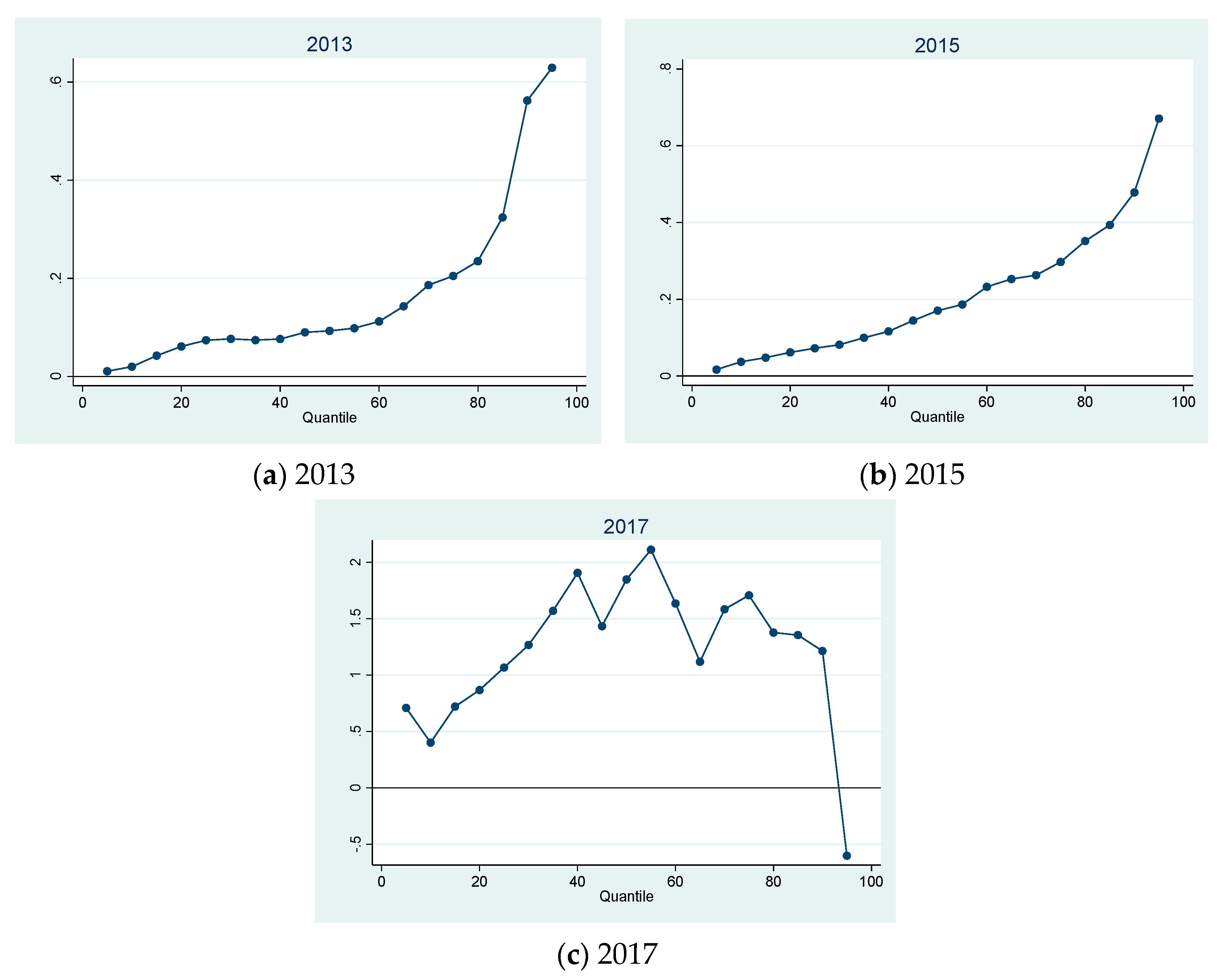
3.1.2. Unconditional Quantile Regression (UQR) Analysis

The above basic regression model can only reflect the impact of financial cognitive level on the overall effect of rural household income with other control variables unchanged, and it fails to reflect the impact of financial cognitive level on the overall distribution of household income. Through empirical observation, we know that the distribution of household income is special and heterogeneous. Therefore, simple linear regression cannot describe the effect of financial cognition on the household income of different groups. This paper further uses the UQR model, based on Equation (2) to explore the impact of financial cognitive level on the overall distribution of rural household income in different years. The corresponding estimation results are shown in

Table 5. Unconditional quantile regression (UQR) results of financial cognitive level on rural household income.

	(1) 2013	(2) 2015	(3) 2017
UQR10th β	0.0197 ** (2.09) 1	0.0369 *** (3.49)	0.400 (1.59)
UQR30th β	0.0763 *** (5.26)	0.0815 *** (5.60)	1.267 *** (4.12)
UQR50th β	0.0927 *** (3.54)	0.170 *** (6.92)	1.847 *** (3.47)
UQR70th β	0.186 *** (4.50)	0.263 *** (6.53)	1.583 ** (2.46)
UQR90th β	0.562 *** (5.81)	0.478 *** (4.68)	1.213 (1.29)
Control variables	yes	yes	yes
Regional fixed effects	yes	yes	yes
N	7046	7046	7046

¹ **, *** represent the significance level of 10%, 5%, and 1%, respectively, and the value in parentheses is the t value.

and Figure 2.

The conclusion obtained in Table 5 is the same as the conclusion obtained by the basic regression model, that is, the level of financial cognition has a positive impact on rural residents’ income. From Table 5, columns (1), (2) and (3) respectively represent the UQR results in 2013, 2015, and 2017 with the addition of control variables and regional fixed effects. Figure 2 depicts the quantile effect. We can see that in different years, the impact of financial cognitive level on rural household income at different quantile levels is different. In both 2013 and 2015, the coefficient of financial cognition gradually increased. In 2017, it fluctuates greatly, and the overall trend is inverted U-shaped. The coefficients at both ends are small and not very significant, and the coefficient reaches the maximum at the 50% quantile level, so the level of financial cognition has the greatest impact on middle-income households.

Before 2017, farmers generally had a relatively shallow understanding of finance, and the threshold for financial services was also high. Due to the large-scale characteristics of the modern financial service industry, low-income families are not the targets of various financial institutions. Therefore, it is difficult for them to enjoy financial services, and it is even more difficult for them to use their wealth management knowledge to increase their wealth. However, high-income families are the key targets of financial institutions, the financial services they enjoy are much better than those of low-income families, so the level of financial cognition has a greater impact on them. After 2017, with the promotion of inclusive finance policies, farmers have a basic understanding of finance, and they can also enjoy basic financial services. Nevertheless, for low-income families, deeper financial knowledge is still of no significant effect, while high-income families have reached a bottleneck in their financial cognition, which means the impact of financial cognition on their household income is in a diminishing trend.

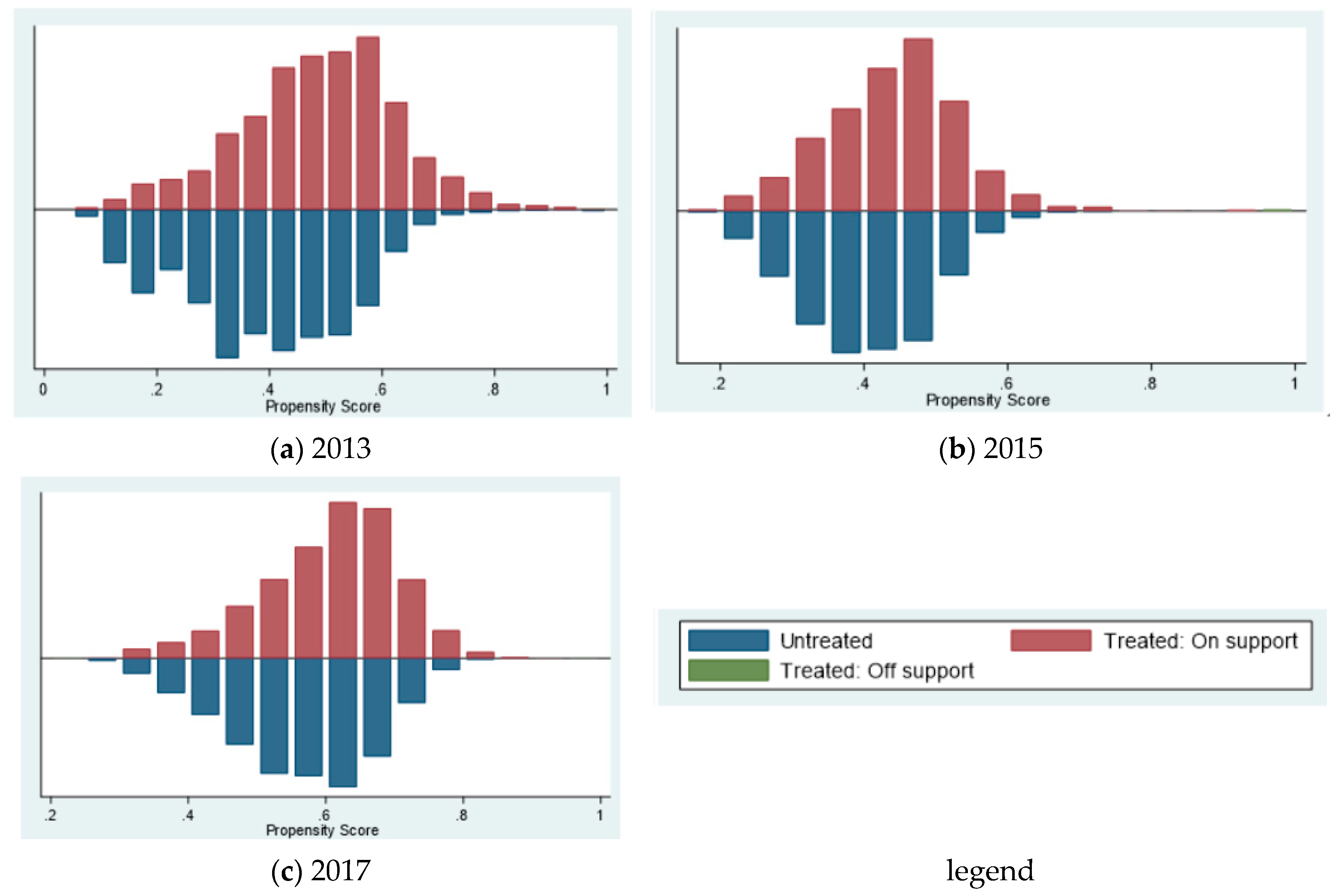
3.2. Robustness Test

When estimating the causal effect between financial cognitive level and household income, we are faced with the basic problem of causal effect inference. We can only observe the household income results of rural residents at the corresponding financial cognitive level, and we cannot observe the causal relationship between the family’s financial cognitive level and other variables. The basic idea of the propensity score matching (PSM) method is that for individuals in the experimental group, it finds the individuals in the control group with similar characteristics to the experimental group in order to match them, and it uses the results of the individuals in the corresponding control group to estimate the counterfactual results of the individuals in the experimental group. PSM solves the problem of selection bias caused by the observed variables in the sample, and further weakens the endogeneity of the model.

The specific implementation steps of PSM are as follows: first, determine the financial cognitive level as the dependent variable, and then according to the value, divide it into two groups where the value greater than the mean is 1 and the value less than the mean is 0. Next, select each characteristic variable of the family as independent variables to perform the binary regression of the logit model. This paper selects the age, gender, marital status, health status, years of education and total family assets as the covariates to provide matching basis for the covariates. All kinds of factor that affect the experimental variables and the outcome variables at the same time should be taken as the basis for the match. This is mainly because, when the tendency score is matched, the accuracy of the match result will be improved by introducing the important factors that affect the outcome variables, the introduction of irrelevant covariates will only make the standard error slightly higher, while the omission of important covariates will cause significant deviation. Finally, after matching the experimental group and the control group, the causal relationship between financial cognitive level and rural household income was determined by the causal effect parameter (ATT) of the two groups. This paper adopts most commonly used four methods to compute ATT as in

Table 6. Propensity score matching (PSM) method balance test.

Matching Method	2013 ATT Difference	2015 ATT Difference	2017 ATT Difference
One-to-one	5.09972472 (1.96) 1	5.52958823 (1.96)	32.7634009 (2.61)
K = 4 Nearest neighbors matching	4.39147759 (2.17)	7.1373086 (2.66)	37.0123294 (3.50)
Radius matching	3.60359892 (2.05)	8.50397007 (3.37)	40.7273265 (4.26)
Kernel matching	3.75708599 (2.14)	8.35412397 (3.31)	40.6649744 (4.25)

¹ The numbers are the ATT difference between treated and untreated after matching, and the value in parentheses is the t value.

.

From Table 6, we can find that the t-value results of all the four methods are bigger than 1.96, which means there are significant ATT differences after matching. This proves that rural household income with high financial cognitive level is significantly more than rural household income with low financial cognitive level.

Limited by the length of the article, this paper only reports report balance test results of the one-to-one matching method, which are shown in

Table 7. PSM method balance test.

Variable	Year	Unmatched	Mean			%Reduced |Bias|	t-Test		V(T)/ V(C)
		Matched	Treated	Untreated	%Bias		t	p > t
asset	2013	U	349.74	216.7	26.1		11.06	0.000	1.78 *1
		M	343.36	333.1	2	92.3	0.71	0.475	0.75 *
	2015	U	389.5	258.34	18.2		7.89	0.000	3.43 *
		M	364.34	343.84	2.8	84.4	1.25	0.211	1.03
	2017	U	384.33	280.39	11.3		4.52	0.000	2.28 *
		M	370.93	364.98	0.6	94.3	0.38	0.703	0.72 *
age	2013	U	50.882	56.033	−43		−17.80	0.000	0.83 *
		M	50.883	50.461	3.5	91.8	1.40	0.162	0.88 *
	2015	U	53.728	57.259	−29.1		−12.01	0.000	0.94
		M	53.718	53.296	3.5	88	1.33	0.182	0.94
	2017	U	55.349	59.269	−32.5		−13.47	0.000	0.91 *
		M	55.336	54.894	3.7	88.7	1.64	0.101	0.85 *
sex	2013	U	0.91898	0.87227	15.3		6.29	0.000	.
		M	0.91893	0.91762	0.4	97.2	0.19	0.852	.
	2015	U	0.89573	0.87032	7.9		3.25	0.001	.
		M	0.8959	0.89929	−1.1	86.7	−0.43	0.668	.
	2017	U	0.90883	0.85916	15.6		6.53	0.000	.
		M	0.90903	0.90806	0.3	98.1	0.15	0.879	.
education	2013	U	7.9922	6.209	54.1		22.32	0.000	0.76 *
		M	7.9895	7.9448	1.4	97.5	0.58	0.563	1.04
	2015	U	7.5142	6.573	27.6		11.39	0.000	0.92 *
		M	7.5137	7.4368	2.3	91.8	0.91	0.365	1.10 *
	2017	U	7.3929	6.3134	31.2		12.95	0.000	0.88 *
		M	7.3943	7.2698	3.6	88.5	1.69	0.091	1
health	2013	U	2.2826	2.0916	14.6		6.10	0.000	1.12 *
		M	2.2811	2.2403	3.1	78.6	1.17	0.244	0.92 *
	2015	U	3.2129	3.0678	14.5		5.99	0.000	0.93 *
		M	3.2126	3.2635	−5.1	65	−1.98	0.048	0.98
	2017	U	3.2009	2.9776	21.5		8.88	0.000	0.96
		M	3.201	3.1969	0.4	98.2	0.18	0.856	1
marriage	2013	U	0.93303	0.87604	19.5		7.97	0.000	.
		M	0.93298	0.93789	−1.7	91.4	−0.78	0.435	.
	2015	U	0.91605	0.89038	8.7		3.56	0.000	.
		M	0.9159	0.90709	3	65.6	1.19	0.233	.
	2017	U	3476.4	3582.6	−5.3		−2.16	0.031	1.16 *
		M	3476.7	3506.7	−1.5	71.8	−0.67	0.503	1.13 *

¹ * represent the significance level of 5%.

and Figure 3.

It can be seen from Table 7 and Figure 3 that in the three years, the treatment groups of all variables have similar mean values before and after matching, while the untreated group has a larger difference. In addition, the p-values are also different before and after matching. In 2013, the deviation was reduced by more than 78%; in 2015, the deviation was reduced by more than 65%; and in 2017, the deviation was reduced by more than 70%, indicating a better matching effect. The results of the balance test prove that the variables selected in this article are appropriate and the model is robust.

4. Further Analysis

4.1. Mechanism Analysis

A large number of scholars have mentioned the impact of inclusive finance on the living standards of farmers, believing that it is the key to reducing poverty and increasing prosperity. This article finds that the level of financial cognition has a significant positive impact on the income of rural households, but the role of inclusive finance in it is still unclear. Since digital financial inclusion is the most effective means of financial inclusion in the era of Internet big data, this paper uses the digital financial inclusion index from the Institute of Digital Finance, Peking University, as an indicator of the implementation degree of digital financial inclusion. It builds model (3) to verify Hypothesis 2:

$$Incom{e}_{it}={\alpha }_{it}+{\beta }_{1it}{f}_{it}+{\beta }_{2it}inde{x}_{it}+{\beta }_{3it}{f}_{it}\times inde{x}_{it}+{\epsilon }_{it},$$

(3)

In Equation (3), $inde{x}_{it}$ represents the digital financial inclusion index of the region where the i-th family is located at time t, and the meanings and calculation methods of other variables are the same as Formula (1). $f_{it}\times inde{x}_{it}$ represents the interaction term between the financial cognitive level and the digital financial inclusion index, focusing on the size and significance of ${\beta }_{3it}$. The regression results are shown in

Table 8. The result of the moderating effect of the digital financial inclusion index.

	(1)		(2)
	Income		Income
${\beta }_1$	−5.259 ***(−11.17) 1	c_${\beta }_1$	1.374 ***(9.84)
${\beta }_2$	5.522 ***(77.13)	c_${\beta }_2$	4.774 ***(113.97)
${\beta }_3$	0.0310 ***(11.59)	c_${\beta }_3$	0.0310 ***(11.59)
α	−880.3 ***(−66.53)	c_α	270.0 ***(120.01)
N	21,138	N	21,138
R-sq	0.391	R-sq	0.391

¹ *** represent the significance level of 1%, and the value in parentheses is the t value.

.

In Table 8, column (1) is the result of the basic moderating effect, column (2) is the result of the moderating effect after centralizing the financial cognitive level and the digital financial inclusion index. Although the coefficient of financial cognitive level in column (1) is negative, it becomes positive after centralization, and all variables are significant under the condition of 1%. Therefore, it can be concluded that the digital financial inclusion index in the region has a positive moderating effect on the impact of financial cognitive level on the income of rural households which is consistent with Hypothesis 2 (H2).

In the information age, financial market activities and digital technology are closely linked. The advantage of digital financial inclusion over traditional financial inclusion lies in the ability to use Internet technology to expand the scope and coverage of financial services. As a result, it is possible to provide financial services for all classes and groups of society in an all-round way. Farmers who are excluded from traditional financial services are the key goal of digital financial inclusion. The higher the implementation level of local digital financial inclusion the greater the coverage, depth of use and digitalization of local digital finance. Correspondingly, local farmers are more likely to enjoy financial services, have a deeper understanding of finance, and use digital finance more frequently. Therefore, local rural residents have a greater advantage compared with backward areas, and they can use their financial cognition more effectively to increase family income.

4.2. Heterogeneity Analysis

Because residents earn income based on external characteristics and personal characteristics, there will be heterogeneity due to differences in external characteristics and personal characteristics. This part validates Hypothesis 3 by testing the heterogeneity of the impact of financial cognition on rural household income.

4.2.1. Regional Heterogeneity

This part starts with external characteristics to analyze regional heterogeneity. The division of this paper is based on the degree of regional development, and the selected indicator is GDP per capita. Considering China’s situation separately, this paper divides GDP per capita equally according to the numerical value into low, medium, and high categories and it also divides the sample into three sub-samples, and then performs regression respectively. The results are shown in

Table 9. Regional heterogeneity regression results.

		(1) Low_GDP	(2) Middle_GDP	(3) High_GDP
		Income	Income	Income
2013	β	−0.017(−0.15) 1	0.360 **(1.99)	0.218 ***(3.34)
	α	23.80 **(2.19)	1.471(0.14)	3.127(0.52)
	Control variables	yes	yes	yes
	N	2097	1194	3755
	R-sq	0.11	0.077	0.055
2015	β	0.117(1.44)	0.378(1.35)	0.251 ***(2.62)
	α	3.583(0.41)	13.06(1.09)	9.339(0.5)
	Control variables	yes	yes	yes
	N	2311	2311	2419
	R-sq	0.198	0.079	0.359
2017	β	0.278(0.37)	0.726(0.97)	1.048 *(1.8)
	α	1096.0 ***(17.7)	1058.9 ***(17.86)	989.1 ***(18.6)
	Control variables	yes	yes	yes
	N	2376	2137	2530
	R-sq	0.206	0.172	0.215

¹ *, **, *** represent the significance level of 10%, 5%, and 1% respectively, and the value in parentheses is the t value.

.

In Table 9, in 2013, the coefficient of financial cognition in areas with low per capita GDP is not significant; in areas with medium per capita GDP, it is significant under the condition of 5%; and in areas with high per capita GDP, the coefficient is significant under the condition of 1%. In 2015 and 2017, the coefficient of per capita GDP is not significant in low and medium regions, and it is significant under the condition of 1% and 10% in high-level regions, respectively. Based on the data of the three years, the impact of financial cognition on rural household income is more significant in areas with high per capita GDP, but less significant in areas with low per capita GDP. The result is consistent with Hypothesis 3 (H3).

Regions with high GDP per capita have more developed overall output levels and more use of Internet technology, and this have certain similarities with regions with high digital financial inclusion indexes. With a broader vision and a relatively better business environment, the financial knowledge of rural residents can act on operating income. They can enjoy higher-quality financial services and have more financial management opportunities, so they can better use financial knowledge to increase their property income and total income accordingly.

4.2.2. Family Asset Heterogeneity

This section starts with the internal characteristics of the family and selects the household holding assets as an indicator. In this paper, according to the quantile of household assets, the sample is divided into low-asset households, lower-middle-asset households, upper-middle-asset households, and high-asset households, and then regressions are performed respectively, and the results are shown in

Table 10. Regression results of family asset heterogeneity.

		(1) Low Assets	(2) Lower Middle Assets	(3) Upper Middle Asset	(4) High Assets
		Income	Income	Income	Income
2013	β	0.0162 (0.34) 1	0.0636 (1.31)	0.125 ** (2.25)	0.394 ** (2.48)
	α	23.40 *** (5.73)	23.53 *** (4.27)	7.9 (1.08)	12.67 (0.61)
	Control variables	yes	yes	yes	yes
	Regional control effect	yes	yes	yes	yes
	N	1761	1762	1762	1761
	R-sq	0.057	0.038	0.046	0.032
2015	β	0.096 * (1.86)	0.0513 (1.1)	0.199 *** (3.43)	1.044 ** (2.16)
	α	20.83 *** (3.38)	27.85 *** (4.23)	12.83 (1.64)	−33.62 (−0.67)
	Control variables	yes	yes	yes	Yes
	Regional control effect	yes	yes	yes	Yes
	N	1759	1760	1761	1761
	R-sq	0.082	0.071	0.061	0.026
2017	β	−0.328 (−0.47)	0.394 (0.49)	0.353 (0.46)	1.038 (1.18)
	α	1223.4 ** (2.37)	353.2 (0.62)	2025.4 *** (3.4)	351.7 (0.58)
	Control variables	yes	yes	yes	yes
	Regional control effect	yes	yes	yes	yes
	N	1760	1760	1762	1761
	R-sq	0.338	0.227	0.173	0.16

¹ *, **, *** represent the significance level of 10%, 5%, and 1%, respectively, and the value in parentheses is the t value.

.

In Table 10, in 2013, the coefficients of financial cognition of the low-asset and the lower-middle-asset are not significant, while the coefficients of financial cognition of the upper-middle-asset and the high-asset are both significant under the condition of 5%. In 2015, the coefficient of financial cognition of the lower-middle-asset is insignificant and low, while the coefficients of financial cognition of the low-asset, the upper-middle-asset, and high-asset are significant under the conditions of 10%, 1%, and 5%, respectively. Although the regression coefficient is not significant in 2017, overall, the coefficients in the three years all increase with the increase in household assets. Therefore, we conclude that the level of financial cognition has a more significant impact on households with more assets, and the impact is also greater which is consistent with Hypothesis 3 (H3).

Families with more assets have more room for asset allocation, stronger risk tolerance and more choices of financial products. Therefore, their financial cognition can play a greater role, which also allows them to earn more income, own more assets, and further improve their investment environment. However, families with fewer assets lack the room to allocate assets, and their risk tolerance is also low owing to lack of asset support, hence their financial opportunities are correspondingly reduced. Even with a high level of financial cognition, the increase in household income is limited.

5. Conclusions

With financial institutions and products constantly emerging, financial cognition has become important human capital. Compared with urban residents, rural residents are in a financially disadvantaged position. Improving financial cognition can enable residents to receive financial information more effectively, identify consumption traps, and rationally allocate their own assets, thereby increasing operating income and property income, and consequently increasing the total family income. In this case, this paper uses an unconditional quantile regression (UQR) model to test the impact of financial cognitive level on rural resident’s income. The following conclusions are obtained.

First, the financial cognitive level promotes the increase of rural household income overall, but this promotion has significant differences at different quantile levels of household income. Research measures the impact of financial literacy training on financial knowledge and behavior, finding that training increased financial literacy of participants, changed their savings and borrowing behavior and had a positive effect on new business start-ups [12,15,53]. However, it fails to have a significant (short-term) impact on income. Also, research has found many factors that improve residents’ income and financial cognitive level [31]. Our research then provides evidence that financial cognitive level can have a significant positive impact on rural household income. In 2013 and 2015, the impact of financial cognitive level on rural household income showed a gradual increase, but in 2017 it fluctuated greatly, showing an overall inverted U-shaped trend and showing that the level of financial cognition has the greatest impact on middle-income households. After 2017, the level of cognition of rural residents reached a basic level. In order to enhance its role in raising income, subsequent inclusive financial policies should be more targeted, especially for low-income families that may require additional measures. Therefore, policy related to improve residents’ financial cognitive level should be given importance.

Furthermore, the digital financial inclusion index in the region has a positive moderating effect on the impact of financial cognition on rural households’ income. Research discovers that digital finance and financial inclusion has several benefits to financial services users, digital finance providers, governments and the economy; notwithstanding, a number of issues still persist which if addressed can make digital finance work better for individuals, businesses and governments [54]. Based on this, we then use a moderating effect model to observe what role of digital financial inclusion plays in the financial cognitive level’s effect on rural household income. With modern information technology, digital financial inclusion uses Internet technology to bring more rural residents into financial services, so that rural residents can more effectively use financial knowledge to increase household income when improving their financial cognition. Therefore, it is suggested that digital technology should be more connected with finance and the depth and width of digital financial inclusion should be increased.

Last but not least, the heterogeneity of the impact of financial cognition on rural households’ income is reflected in two aspects: region and household assets. The impact of financial cognition on rural household income is more significant in areas with high per capita GDP, and less significant in areas with low per capita GDP. In more developed regions, the digital financial inclusion index is relatively high, and the financial environment of local rural residents is better. Therefore, the formulation of policies also needs to consider the development of the region. In addition, the level of financial cognition has a more significant impact on high-asset households, and the impact is also greater. The financial cognitive level of rural residents can play a better role in increasing income with the support of high assets hence they can further increase their own assets. There is a mutually reinforcing relationship between the two. Without the support of high assets, the financial cognitive level of rural residents is still limited. Therefore, policies also need to consider the difference between rich and poor families.

References

1. Nam, S. Cognitive capitalism, free labor, and financial communication: A critical discourse analysis of social media IPO registration statements. Inf. Commun. Soc. 2020, 23, 420–436. [Google Scholar] [CrossRef]
2. Li, T.; Liao, G. The Heterogeneous Impact of Financial Development on Green Total Factor Productivity. Front. Energy Res. 2020, 8, 29. [Google Scholar] [CrossRef] [Green Version]
3. Zhong, J.; Li, T. Impact of Financial Development and Its Spatial Spillover Effect on Green Total Factor Productivity: Evidence from 30 Provinces in China. Math. Probl. Eng. 2020, 2020, 5741387. [Google Scholar] [CrossRef] [Green Version]
4. Li, Z.; Wang, Y.; Huang, Z. Risk Connectedness Heterogeneity in the Cryptocurrency Markets. Front. Phys. 2020, 8, 243. [Google Scholar] [CrossRef]
5. Xu, S. International comparison of green credit and its enlightenment to China. Green Financ. 2020, 2, 75–99. [Google Scholar] [CrossRef]
6. Li, Z.; Dong, H.; Floros, C.; Charemis, A.; Failler, P. Re-examining Bitcoin Volatility: A CAViaR-based Approach. Emerg. Mark. Financ. Trade 2021. [Google Scholar] [CrossRef]
7. Tan, Y.; Li, Z.; Liu, S.; Nazir, M.I.; Haris, M. Competitions in different banking markets and shadow banking: Evidence from China. Int. J. Emerg. Mark. 2021. [Google Scholar] [CrossRef]
8. Wen, F.; Cao, J.; Liu, Z.; Wang, X. Dynamic volatility spillovers and investment strategies between the Chinese stock market and commodity markets. Int. Rev. Financ. Anal. 2021, 76, 101772. [Google Scholar] [CrossRef]
9. Mouna, A.; Anis, J. Financial literacy in Tunisia: Its determinants and its implications on investment behavior. Res. Int. Bus. Financ. 2017, 39, 568–577. [Google Scholar] [CrossRef]
10. Croce, A.; Ughetto, E.; Cowling, M. Investment Motivations and UK Business Angels’ Appetite for Risk Taking: The Moderating Role of Experience. Br. J. Manag. 2019, 31, 728–751. [Google Scholar] [CrossRef]
11. Wickstrom, K.A.; Klyver, K.; Cheraghi-Madsen, M. Age effect on entry to entrepreneurship: Embedded in life expectancy. Small Bus. Econ. 2020, 1–20. [Google Scholar] [CrossRef]
12. Lusardi, A.; Michaud, P.-C.; Mitchell, O.S. Optimal Financial Knowledge and Wealth Inequality. J. Political Econ. 2017, 125, 431–477. [Google Scholar] [CrossRef] [Green Version]
13. Zhu, A.Y.F.; Yu, C.W.M.; Chou, K.L. Improving Financial Literacy in Secondary School Students: An Randomized Experiment. Youth Soc. 2021, 53, 539–562. [Google Scholar] [CrossRef]
14. Evgenii, G.; Aleksandra, C. Saving behavior and financial literacy of Russian high school students: An application of a copula-based bivariate probit-regression approach. Child. Youth Serv. Rev. 2021, 127, 106122. [Google Scholar]
15. Finke, M.S.; Howe, J.S.; Huston, S.J. Old Age and the Decline in Financial Literacy. Manag. Sci. 2017, 63, 213–230. [Google Scholar] [CrossRef]
16. MacLeod, S.; Musich, S.; Hawkins, K.; Armstrong, D.G. The growing need for resources to help older adults manage their financial and healthcare choices. BMC Geriatr. 2017, 17, 84. [Google Scholar] [CrossRef] [PubMed] [Green Version]
17. Anderson, A.; Baker, F.; Robinson, D.T. Precautionary savings, retirement planning and misperceptions of financial literacy. J. Financ. Econ. 2017, 126, 383–398. [Google Scholar] [CrossRef] [Green Version]
18. Demirtas, Y.E.; Kececi, N.F. The efficiency of private pension companies using dynamic data envelopment analysis. Quant. Financ. Econ. 2020, 4, 204–219. [Google Scholar] [CrossRef]
19. Toosi, N.R.; Voegeli, E.N.; Antolin, A.; Babbitt, L.G.; Brown, D.K. Do Financial Literacy Training and Clarifying Pay Calculations Reduce Abuse at Work? J. Soc. Issues 2020, 76, 681–720. [Google Scholar] [CrossRef]
20. Meyll, T.; Pauls, T. The gender gap in over-indebtedness. Financ. Res. Lett. 2019, 31, 398–404. [Google Scholar] [CrossRef]
21. Morshadul, H.; Thi, L.; Ariful, H. How does financial literacy impact on inclusive finance? Financ. Innov. 2021, 7, 1–23. [Google Scholar]
22. Grohmann, A.; Kluehs, T.; Menkhoff, L. Does financial literacy improve financial inclusion? Cross country evidence. World Dev. 2018, 111, 84–96. [Google Scholar] [CrossRef] [Green Version]
23. Naz, M.; Iftikhar, S.F.; Fatima, A. Does financial inclusiveness matter for the formal financial inflows? Evidence from Pakistan. Quant. Financ. Econ. 2020, 4, 19–35. [Google Scholar] [CrossRef]
24. Coibion, O.; Gorodnichenko, Y.; Kudlyak, M.; Mondragon, J. Greater Inequality and Household Borrowing: New Evidence from Household Data. J. Eur. Econ. Assoc. 2020, 18, 2922–2971. [Google Scholar] [CrossRef]
25. Szymborska, H.K. Wealth structures and income distribution of US households before and after the Great Recession. Struct. Chang. Econ. Dyn. 2019, 51, 168–185. [Google Scholar] [CrossRef]
26. Larrimore, J.; Mortenson, J.; Splinter, D. Household Incomes in Tax Data Using Addresses to Move from Tax-Unit to Household Income Distributions. J. Hum. Resour. 2021, 2, 600–631. [Google Scholar] [CrossRef] [Green Version]
27. Nicolini, E.A.; Palencia, F.R. Decomposing income inequality in a backward pre—Industrial economy. Econ. Hist. Rev. 2016, 69, 747–772. [Google Scholar] [CrossRef]
28. Markkanen, S.; Braeckman, J.P.; Souvannaseng, P. Mapping the evolving complexity of large hydropower project finance in low and lower-middle income countries. Green Financ. 2020, 2, 151–172. [Google Scholar] [CrossRef]
29. Murayama, Y. Inequality, mobility, and growth. Natl. Account. Rev. 2019, 1, 62–70. [Google Scholar] [CrossRef]
30. Sukharev, O.S. Structural analysis of income and risk dynamics in models of economic growth. Quant. Financ. Econ. 2020, 4, 1–18. [Google Scholar] [CrossRef]
31. Aguila, E.; Park, J.H.; Vega, A. Living Arrangements and Supplemental Income Programs for Older Adults in Mexico. Demography 2020, 57, 1345–1368. [Google Scholar] [CrossRef]
32. Hickey, G.M.; Pouliot, M.; Smith-Hall, C.; Wunder, S.; Nielsen, M.R. Quantifying the economic contribution of wild food harvests to rural livelihoods: A global-comparative analysis. Food Policy 2016, 62, 122–132. [Google Scholar] [CrossRef]
33. Zhang, L.; Feng, S.; Heerink, N.; Qu, F.; Kuyvenhoven, A. How do land rental markets affect household income? Evidence from rural Jiangsu, PR China. Land Use Policy 2018, 74, 151–165. [Google Scholar] [CrossRef]
34. Davis, B.; Di Giuseppe, S.; Zezza, A. Are African households (not) leaving agriculture? Patterns of households’ income sources in rural Sub-Saharan Africa. Food Policy 2017, 153–174. [Google Scholar] [CrossRef] [PubMed] [Green Version]
35. Takada, S.; Morikawa, S.; Idei, R.; Kato, H. Impacts of improvements in rural roads on household income through the enhancement of market accessibility in rural areas of Cambodia. Transportation 2021, 1–25. [Google Scholar] [CrossRef]
36. Aryo, S.G.; Jeffrey, D.; Qing, L.; Nigar, N.; Firman, W. Tobacco or not tobacco: Predicting farming households’ income in Indonesia. Tob. Control 2021, 30, 320–327. [Google Scholar]
37. McNelis, P.D.; Yoshino, N. Household Income Dynamics in A Lower-Income Small Open Economy: A Comparison of Banking and Crowdfunding Regimes. Singap. Econ. Rev. 2018, 63, 147–166. [Google Scholar] [CrossRef]
38. Abdullah, A.N.M.; Stacey, N.; Garnett, S.T.; Myers, B. Economic dependence on mangrove forest resources for livelihoods in the Sundarbans, Bangladesh. For. Policy Econ. 2016, 64, 15–24. [Google Scholar] [CrossRef]
39. Angelsen, A.; Jagger, P.; Babigumira, R.; Belcher, B.; Hogarth, N.J.; Bauch, S.; Boerner, J.; Smith-Hall, C.; Wunder, S. Environmental Income and Rural Livelihoods: A Global-Comparative Analysis. World Dev. 2014, 64, S12–S28. [Google Scholar] [CrossRef] [Green Version]
40. Chen, S.; Luo, E.-g.; Alita, L.; Han, X. Impacts of formal credit on rural household income: Evidence from deprived areas in western China. J. Integr. Agric. 2021, 20, 927–942. [Google Scholar] [CrossRef]
41. Arouri, M.; Ben Youssef, A.; Nguyen, C. Does urbanization reduce rural poverty? Evidence from Vietnam. Econ. Model. 2017, 60, 253–270. [Google Scholar] [CrossRef] [Green Version]
42. Igwe, P.A.; Rahman, M.; Odunukan, K.; Ochinanwata, N.; Egbo, O.P.; Ochinanwata, C. Drivers of diversification and pluriactivity among smallholder farmers-evidence from Nigeria. Green Financ. 2020, 2, 263–283. [Google Scholar] [CrossRef]
43. Peng, G.; Liu, F.; Lu, W.; Liao, K.; Tang, C.; Zhu, L. A spatial-temporal analysis of financial literacy in United States of America. Financ. Res. Lett. 2018, 26, 56–62. [Google Scholar] [CrossRef]
44. Carpena, F.; Cole, S.; Shapiro, J.; Zia, B. The ABCs of Financial Education: Experimental Evidence on Attitudes, Behavior, and Cognitive Biases. Manag. Sci. 2019, 65, 346–369. [Google Scholar] [CrossRef] [Green Version]
45. OECD INFE. Measuring Financial Literacy: Core Questionnaire in Measuring Financial Literacy: Questionnaire and Guidance Notes for Conducting an Internationally Comparable Survey of Financial Literacy; OECD: Paris, France, 2020. [Google Scholar]
46. Song, X.; Guo, H. Influence Factors of the Urban-rural Residents’ Income Gap: A Restudy with the Digital Inclusive Finance. In Proceedings of the 2017 4th International Conference on Business, Economics and Management, Qingdao, China, 16–17 November 2017; p. 7. [Google Scholar]
47. Li, Z.; Chen, L.; Dong, H. What are bitcoin market reactions to its-related events? Int. Rev. Econ. Financ. 2021, 73, 1–10. [Google Scholar] [CrossRef]
48. Jiang, Y.; Tian, G.; Wu, Y.; Mo, B. Impacts of geopolitical risks and economic policy uncertainty on Chinese tourism-listed company stock. Int. J. Financ. Econ. 2020. [Google Scholar] [CrossRef]
49. Gan, L.; Yin, Z.; Tan, J. Report on the Development of Household Finance in Rural China (2014); Springer: Singapore, 2016. [Google Scholar]
50. Guo, F.; Wang, J.; Wang, F.; Kong, T.; Zhang, X.; Zhiyun, C. Measuring China’s Digital Financial Inclusion: Index Compilation and Spatial Characteristics. China Econ. Q. 2020, 19, 1401–1418. [Google Scholar]
51. Koenker, R.; Bassett, G. Regression Quantiles. Econometrica 1978, 46, 33–50. [Google Scholar] [CrossRef]
52. Firpo, S.; Fortin, N.M.; Lemieux, T. Unconditional Quantile Regressions. Econometrica 2009, 77, 953–973. [Google Scholar] [CrossRef] [Green Version]
53. Sayinzoga, A.; Bulte, E.H.; Lensink, R. Financial Literacy and Financial Behaviour: Experimental Evidence from Rural Rwanda. Econ. J. 2016, 126, 1571–1599. [Google Scholar] [CrossRef]
54. Ozili, P.K. Impact of digital finance on financial inclusion and stability. Borsa Istanb. Rev. 2018, 18, 329–340. [Google Scholar] [CrossRef]
Figure 1. The normal quantile map of rural household income in different years that (ac) describe the situation in 2013, 2015, and 2017, respectively.
Agronomy 11 01813 g001
Figure 2. The quantile effect of financial cognitive level on rural household income in different years that (ac) describe the situation in 2013, 2015, and 2017, respectively.
Agronomy 11 01813 g002
Figure 3. PSM method balance test chart: (a) Describe 2013; (b) Describe 2015; (c) Describe 2017.
Agronomy 11 01813 g003