A Parametric Model for Local Air Exchange Rate of Naturally Ventilated Barns

Abstract

With an increasing number of naturally ventilated dairy barns (NVDBs), the emission of ammonia and greenhouse gases into the surrounding environment is expected to increase as well. It is very challenging to accurately determine the amount of gases released from a NVDB on-farm. Moreover, control options for the micro-climate to increase animal welfare are limited in an NVDB at present. Both issues are due to the complexity of the NVDB micro-environment, which is subject to temporal (such as wind direction and temperature) and spatial (such as openings and animals acting as airflow obstacles) fluctuations. The air exchange rate (AER) is one of the most valuable evaluation entities, since it is directly related to the gas emission rate and animal welfare. In this context, our study determined the general and local AERs of NVDBs of different shapes under diverse airflow conditions. Previous works identified main influencing parameters for the general AER and mathematically linked them together to predict the AER of the barn as a whole. The present research study is a continuation and extension of previous studies about the determination of AER. It provides new insights into the influence of convection flow regimes. In addition, it goes further in precision by determining the local AERs, depending on the position of the considered volume inside the barn. After running several computational fluid dynamics (CFD) simulations, we used the statistical tool of general linear modeling in order to identify quantitative relationships between the AER and the following five influencing parameters, the length/width ratio of the barn, the side opening configuration, the airflow temperature, magnitude and incoming direction. The work succeeded in taking the temperature into account as a further influencing parameter in the model and, thus, for the first time, in analysing the effect of the different types of flow convection in this context. The resulting equations predict the barn AER with an $R^2$ equals 0.98 and the local AER with a mean $R^2$ equals around 0.87. The results go a step further in the precise determination of the AER of NVDB and, therefore, are of fundamental importance for a better and deeper understanding of the interaction between the driving forces of AER in NVDB.

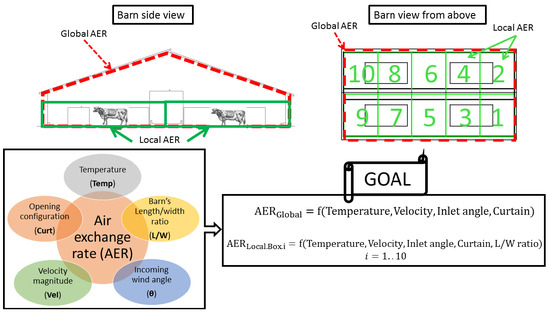
1. Introduction

Animal husbandry must be animal- and environmentally friendly to be socially accepted and sustainable [1]. The air exchange rate (AER) and the direction of air movement are key parameters in this context to evaluate animal housing with regard to animal welfare [2] and environmental compatibility [3]. The AER is defined as the quotient of the total volume airflow flow entering a room and the volume of this room. It quantifies the theoretical air replacement per time unit. Livestock producers have two options for removing polluting gases, moisture and heat from animal houses—mechanical and natural ventilation. The economically highly relevant dairy cows sector typically uses naturally ventilated barns (NVB) across Europe—a housing system which is partly also used for poultry or pigs [4]. The main advantage of these buildings is their energy-saving property since, in general, natural ventilation does not require electrical energy to operate fans or a furnace. However, in many cases, fans support natural ventilation under hot climate conditions. The desire for maximal animal welfare and minimal environmental impact results in a conflict of goals, since the emission rate (ER) is coupled with the AER: $ER=C_{0}AER{V}_t$, with $C_0$ (in m g m${}^{-3}$) as the concentration of a pollutant gas inside the barn and $V_t$ (in m${}^3$) as the volume of the space. Thus, to only increase the global AER of a barn to improve the animal welfare results in an increase in the balance-dependent emissions of an NVB. In contrast, local AER in animal-occupied spaces must be selectively modified.

Computational fluid dynamics (CFD) methods are applied with increasing frequency in agricultural research to model the interior air flow in barns and greenhouses [5,6]. Due to the theoretically unlimited spatial and temporal resolution and the defined boundary conditions, they are an optimal complement to measurements and permit deep insights into the development of airflow patterns [7]. The effect of individual stimuli (e.g., building design or thermal input) on the airflow patterns can be investigated in detail in order to develop strategies for the precise control of local AER. The numerical models rely on discretization schemes and how well the geometric models are divided into tiny parts called cells (meshing). Model depth and accuracy depends on the research question, the computational power and the chosen parametrizations of unresolved processes [5,8].

The description of turbulence is of particular relevance. In agriculture, numerical flow simulations typically rely on the Reynolds Averaged Navier–Stokes (RANS) approach [9]. It provides a good cost–benefit ratio and has been used in scientific and industrial applications for more than 40 years. State-of-the-art CFD models of air flow through livestock houses include inflow modeling and the estimation of AER [10,11,12]. In a pre-study published in January 2021 [13], we showed that it is possible to model animals as a porous media that reproduce the pressure drop and heat transfer relatively well (less than 6% error). The advantage of using porous media is the gained computing time, which is at least 70% compared to a numerical simulation with 3D modeled animals. The combination of the RANS with the porous media made the present parametric study timely realizable, in such a way that 243 simulations have been realized in only three months on 30 CPUs. The number of simulations comes from the fact that we considered three “values” for three of the parameter chosen for the study and nine “values” for the other two (coupled) parameters ($3\times 3\times 9$ = 243). One of the latest studies on this topic, conducted by Yi et al. [12], explored the influences and possible interactions between the opening ratio, the building length-to-width ratio, the wind speed and the wind direction. They found that the influence of the length-to-width ratio was negligible, while the AER was significantly affected by the wind speed, the wind direction and interaction effects between each two of the three factors. However, the study was limited to the global AER and the influence of convective flow regimes was not investigated.

For this reason, the present manuscript, which follows the same direction, wants to enlarge the scope of the AER prediction by investigating the following hypothesis:

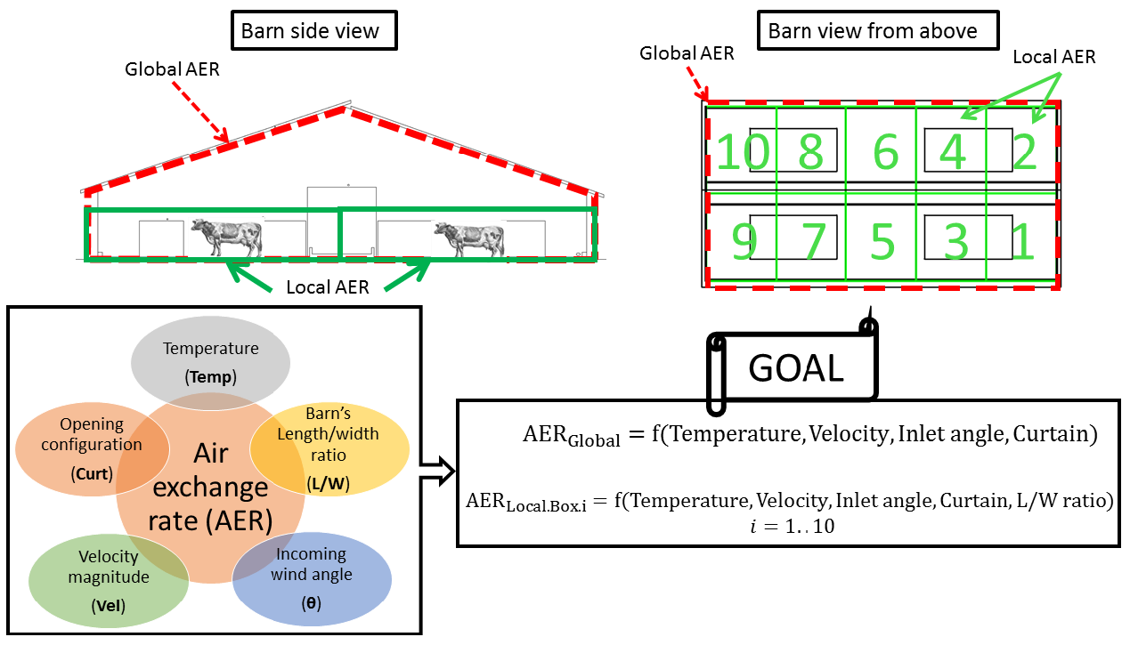
• Under the same boundary conditions, local AERs can show considerably different behavior, first, depending on the position inside the barn and second, in comparison with the global AER.
• The interaction between the temperature and velocity (which is directly related to the flow convection type) has a strong influence on the global and local AERs, as well as the interactions between other pre-cited parameters confirmed in previous studies.

The confirmation of those hypothesizes represents the novelty of the present work. The present work is subdivided as follow. First, the CFD numerical model will be presented in detail. Then, the parameters and the motivations behind their choices are explained. Afterwards, the corresponding scheme and the method used to run and automatize the simulations are exposed. The next part deals with the evaluation method for global and local AERs. The last part of the methodology and materials segment introduces the general linear model as the chosen statistical method for the interpretation of the results. In the result section, the equations with the highest $R^2$ describing the AERs are proposed, following a comparison with the previous findings. Finally, we present conclusion of the present work and we offer ways to possibly expand on the topic in future.

2. Methodology and Materials

2.1. CFD Model

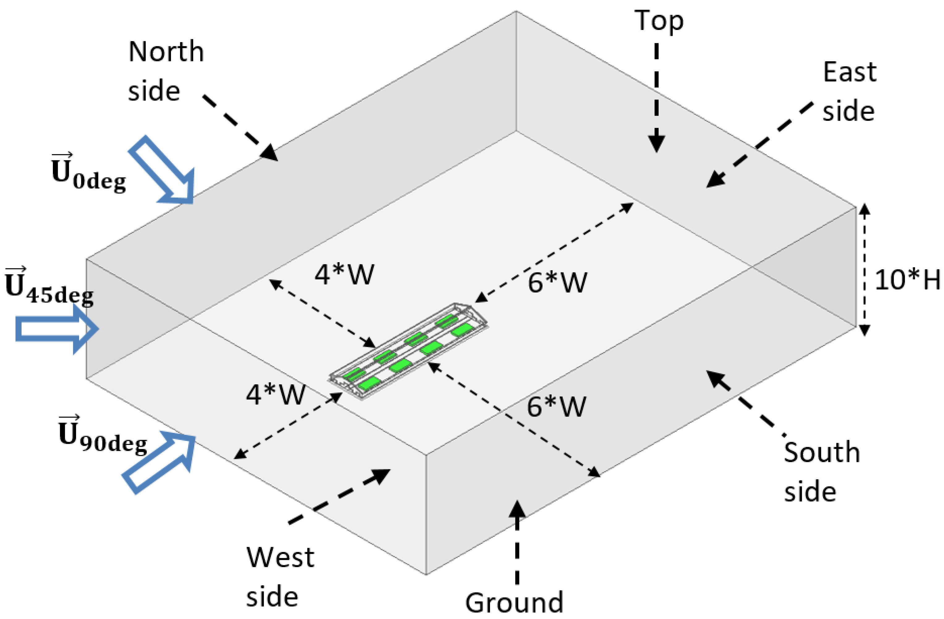
2.1.1. Domain and Boundary Condition

The present study is based on the same numerical model used in [13]. The dimensions of the numerical domain are summarized in Figure 1. The characteristic lengths, such the width W and the height H, are based on the ATB barn sizes in Northern Germany [14], W = 34.2 m, H = 11.5 m.

The inlet velocity describes an atmospheric boundary layer (ABL) profile with the equation [15]:

$$\begin{array}{c}\hfill U\left(y\right)=U_{ref}{\left(\frac{y}{y_{ref}}\right)}^{\alpha }\end{array}$$

(1)

Here, $U\left(y\right)$ is the inlet velocity profile (in m s${}^{-1}$), $U_{ref}$ is the chosen velocity (in m s${}^{-1}$) at the height $y_{ref}$ (in m) and $\alpha$ is a power coefficient (dimensionless). The value of $\alpha$ = 0.16 was extracted from wind tunnel measurements. The value chosen for the ground roughness was 0.068 m, which corresponded to a moderately rough terrain and helped to conserve the form of the ABL profile [11]. The distances 4 W for the inlet and 6 W for the outlet were chosen so that the boundary conditions are far away enough to not influence the flow inside the barn. The domain boundary conditions were set in relation to the inflow air angle.

Table 1. Boundary conditions corresponding to airflow directions.

Inflow Direction	North Side	South Side	West Side	East Side
0$°$	velocity inlet	pressure outlet	Wall	Wall
45$°$	velocity inlet	pressure outlet	velocity inlet	pressure outlet
90$°$	Wall	wall	velocity inlet	pressure outlet

shows the details.

The AOZ of cows, which depict flow obstacles and heat sources, is modelled as a porous medium. The dimensions of the each AOZ are L${}_{AOZ}$ = W/2, W${}_{AOZ}$ = W/4 and disposed as shown in green in Figure 1. According to the density 2.4 m${}^2$ cow${}^{-1}$ (taken from the aforementioned barn in Northern Germany; for a detailed barn description, see, e.g., Janke et al. [14]); the number of cows for the AOZ dimensions is 33. Using the method descripted in Doumbia et al. [13], the AOZ was replaced by a porous medium with the corresponding pressure drop (in the three main directions) and heat transfer functions extracted from the 33 cows 3D geometry (randomly distributed with a ratio of 60% lying and 40% standing) numerical simulation. Based on this method, the porous medium reproduced a pressure drop and heat transfer with fewer than 6% errors, but can significantly reduce the computation time by up to 70% in comparison with its corresponding 3D cows model.

2.1.2. Numerical Solver and Mesh

The numerical settings (solvers, turbulence model, meshing) are same as in [13]. While the most important information will be summarized here, we suggest that the reader looks into the pre-cited paper for more details. The simulations were run in steady state (time independent). The pressure velocity-coupling scheme was set to coupled to improve convergence. The spatial discretization schemes were kept standard (ANSYS, 2019), i.e., second-order upwind for the momentum and the energy, first-order upwind for the turbulent kinetic energy and the specific dissipation rate, second-order for the pressure. The turbulence model chosen for the study is the k-omega model. The mesh is composed of unstructured (around the barn) and structured (for the domain) (see [11]). Based on the mesh convergence performed in Doumbia et al. [13], the chosen cell sizes were 0.4 m for the refinement body and 0.8 m for the barn, with a growth rate of 1.2. The total cell number varied from 12 (for the barn $L/W=2$) to 19 million (for the barn $L/W=4$). The corresponding computing time on 30 CPUs varied from 2 to 4 h for one simulation, depending on the cell number.

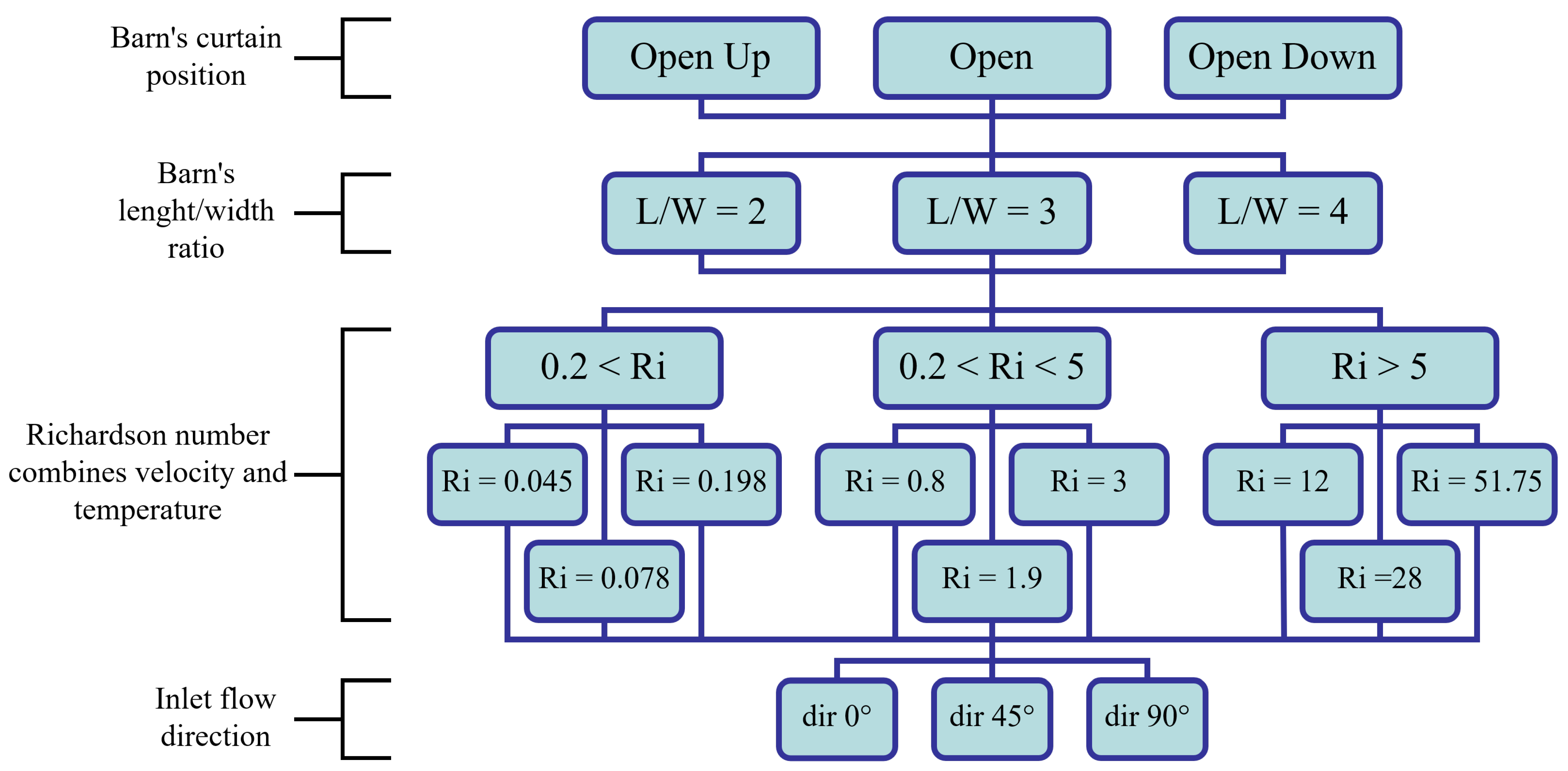
2.2. Parameters

In this section, the parameters chosen for the study, as well as the reasons for their choice, will be presented in detail. After an extensive look at the literature and based on the ATB of previous studies [11,12], the following parameters were retained as potentially having the most influence on the AER: air velocity magnitude ($Vel$), wind direction ($\theta$), temperature gradient between the cows and the ambient air ($Temp$), length-to-width ratio of the barn ($L/W$) and barn curtain position ($Curt$). Wind obviously plays an important role in the air exchange of a NVDB. In this context, [11] noticed that each incoming air direction produces a particular pattern inside the barn, with a tendency towards higher values at the windward side of the building. See Figure 1 for the three chosen air incident angles, 0$°$, 45$°$ and 90$°$. We chose to retain the $L/W$ ratio for two main reasons, even if one study, the conclusions of Yi et al. [12], suggested that it had negligible influence on the AER. First, since there is a variety of NVDBs $L/W$ ratios [16], we want to test if the same conclusion applied to the local AER. Second, the influence of the interaction of $L/W$ with the temperature (a newly introduced parameter) is still unknown. For the study, the values $L/W$ = 2 (Figure 2a), 3 (Figure 2b) or 4 (Figure 2c) were retained.

The barn curtain position (or side opening ratio), $Curt$, has been already reported as an important impact on the AER, Yi et al. [17] and Yi et al. [12], Gebremedhin et al. [18], Saha et al. [19] stated that AER of some configurations can be up to three times the AER of the standard configuration. The curtain positions retained here are totally open (no curtain, Figure 2a), open up (curtain from the floor until the middle of the opening height, Figure 2b) and open down (curtain from the roof until the middle of the opening height, Figure 2c).

The velocity magnitude and the temperature gradient, when combined, can create different convection flow regimes. The Richardson number Ri, which is the ratio of the buoyancy forces and the kinetic forces, was used to distinguish between the three types of convection [20]

$$\begin{array}{cc}\hfill Ri& =\frac{Gr}{{Re}^2}\hfill \end{array}$$

(2)

$$\begin{array}{cc}\hfill Gr& =g\beta L_{HG}^3\frac{(T_s-T_{in})}{{\nu }^2}\hfill \end{array}$$

(3)

$$\begin{array}{cc}\hfill Re& =\frac{u{L}_{HG}}{\nu }\hfill \end{array}$$

(4)

$$\begin{array}{cc}\hfill \beta & =\frac{1}{\frac{T_s+T_{in}}{2}}\hfill \end{array}$$

(5)

$$\begin{array}{cc}\hfill L_{HG}& =\frac{Wg+324.52}{417.5}\hfill \end{array}$$

(6)

where Gr is the Grashof number and Re is the Reynolds number (both dimensionless); L${}_{HG}$ (=2.4 m in our case) the characteristic length is the heart girth used by Wang et al. [21] and based on the cow weight Wg (=675 Kg, as the mean cow weight from our ATB barn in Dummersdorf [22]), T${}_s$ (=311.15 K) is the cow or solid temperature [23], T${}_{in}$ (in K) is the inlet air temperature, $\nu$ (=1.652 × 10${}^{-5}$ m${}^2$ s${}^{-1}$) is the kinematic viscosity, U (in m s${}^{-1}$) is the inlet velocity and g (= 9.81 m s${}^{-2}$) is the gravitational acceleration. The Ri number is related to the convection type as the following. When Ri > > 1, the buoyancy forces represented by the Grashof number (Gr) prevail over the kinetic forces represented by the Reynolds number. When $Ri\approx 1$, the buoyancy forces are on par with the kinetic forces. In addition, for Ri < < 1, the kinetic forces are dominant. The range and limits 0.2–5 for the mixed convection are extracted from [20] as practical values. The nine values of Richardson number were considered to cover the three types of convection and the different seasons of the year, recapitulated in

Table 2. Type of convective heat transfer and Ri values.

	Ri Cases
Type of Convection	Forced			Mixed			Natural
Ri domain	Ri < 0.2			0.2 < Ri < 5			Ri > 5
Ri values	Ri = 0.048	Ri = 0.078	Ri = 0.198	Ri = 0.8	Ri = 1.9	Ri = 3	Ri = 12	Ri = 28	Ri = 51.75
T${}_{air}$ ($°$C)	32	30	22	18	15	10	7	0	−2
U${}_{ref}$ (m s${}^{-1}$)	3.2	2.8	2.5	1.4	0.97	0.85	0.45	0.33	0.25
Season	Summer			Fall-Spring			Winter

.

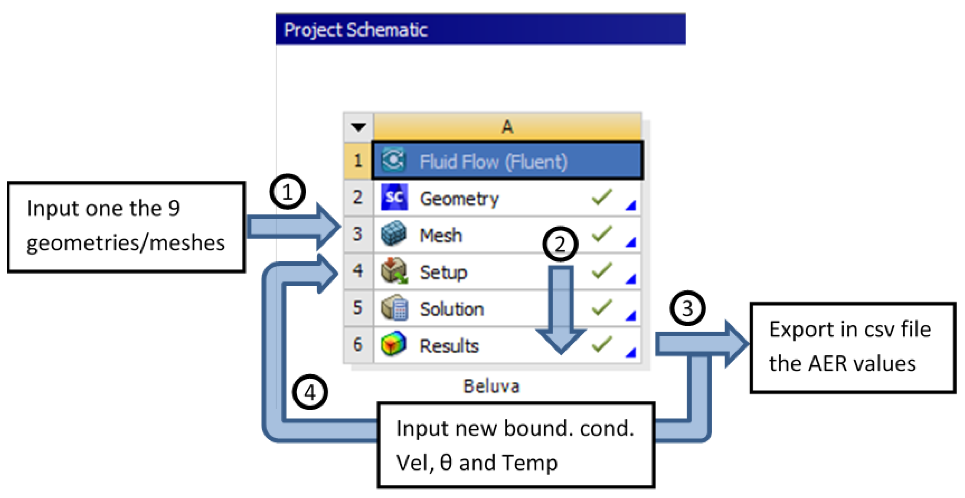
2.3. Simulation Scheme and Automatizing Details (with Ansys Fluent and Python)

Figure 3 shows the scheme of the parameters composition and their corresponding values. Due to this composition and the resulting diverse cases, the study required an enormous number of CFD simulations. The use of the RANS model with the porous model, instead of the RANS with fully resolved cows, reduces the computational time enormously, but the number of resulting cases is still very high. It was obvious that manually launching each simulation run with manual parameter settings was not an option. For this reason, we used the user interface (UI) provided by ANSYS and developed a fully automated workflow based on a combination with Python (3.6.4) and BATCH scripts. We coupled a Python homemade script to modify a so-called ANSYS journal file to provide the parameter values for the simulation. The journal records ANSYS commands in a text user interface (TUI) format and can be re-run to automatically execute the recorded commands.

The ANSYS internal workflow is described in Figure 4. The main script first called out ANSYS and implemented the mesh (already prepared by the user) in step 1. A loop was executed for this mesh. In the loop, the journal file was modified according to the boundary conditions ($Vel$, $\theta$ and $Temp$), the CFD simulation was executed in ANSYS Fluent (setup and solution) and, as a second step, the post-processing (analysis of the simulation results) was performed in CFD-Post. In step 3, the AER of the barn and the local AERs were calculated internally in ANSYS and then written to a CSV file. In step 4, the journal was modified by implementing new boundary conditions and then the script returned to step 2. The loop (steps 2-3-4) was run until the simulations for all boundary conditions $Vel,\theta$ and $Temp$ were completed. Next, one of the nine cases (3 $\times L/W\times$ 3· curtain positions = 9 possible geometry cases) were run in step 1, and so on. By fully automating the process, a significant time-saving was achieved and the probability of human typing errors was drastically reduced.

2.4. AER Evaluation

The AER was evaluated globally, for the barn as a whole, and locally, for each box of the subdivision. To gain a deeper understanding of the local AER, we decided to virtually divide the barn into 10 parts (or volumes) relative to the barn sizes (L/W = 2, 3 and 4). The dimensions of the boxes are as follows: L${}_{Box,L/W=i}$ = L${}_{L/W=i}$/5, W${}_{Box}$ = W/2, H${}_{Box}$ = 2 × H${}_{AOZ}$ = 3.2 m. These virtual subdivisions can be observed in Figure 5. We numbered the boxes to identify their position relative to the incoming airflow. The AER is calculated through the equation:

$$\begin{array}{c}\hfill AER=\frac{3600\dot{V}}{V_{AER}}\end{array}$$

(7)

Here, AER is the air exchange rate of the volume $V_{AER}$ (in h${}^{-1}$), $\dot{V}$ is the sum of volume flow entering $V_{AER}$ (in m${}^3$ s${}^{-1}$) and $V_{AER}$ the considered volume for AER evaluation (in m${}^3$). $V_{AER}$ can be the volume of the whole barn or the volume of a single box.

2.5. Tools and Methods for Statistical Analysis (with R)

The software we employed in this study is the open-source software R for calculations and statistical analysis. In the following paragraphs, the reasoning for the use of the principal component analysis and the general linear model are presented, together with the necessary vocabulary for the study. We would like the readers to keep in mind that deepening this topic is out of the scope of the present work. We refer the readers to the wide statistical analysis literature for further details.

2.5.1. Principal Component Analysis

The initial idea of principal component analysis (PCA) is dimensionality reduction (i.e., explaining as much of the data variance as possible, with the lowest possible number of variables by conducting an orthogonal projection of the data). At present, this statistical procedure is often used for data clustering. In our case, it will help to observe if and how the AERs form clouds. The objective is to extract valuable patterns by displaying the data in the function of new unrelated parameters, the principal components (PCs). This can be done by transposing the data into a new orthogonal coordinate system in which the first principal component is orthogonal to the second principal component, which itself is orthogonal to the third principal component (if any) and so on (if any). The principal components are combinations of the parameters/variables influencing the data.

2.5.2. General Linear Model (GLM)

The GLM is a regression method that determines only one variable (called the dependent variable, which, here, is the AER) based on other variables (called independent variables, which, for us, are the five parameters), which can be multiplied with each other within the terms of a polynomial-type equation; see the equation below. For the independent variables, it is important to distinguish between the continuous variables and the factor variable. While it is easy to understand the meaning of the continuous variables, the factor variable needs more explanation. Factor variables refer to different categories and are used for qualitative description instead of a quantitative ranking. They have different levels (for example, in our case, the levels of the curtain positions are open, open up and open down) with one of them set as the standard; see

Table 3. Boundary conditions corresponding to flow directions.

Parameter Description	Velocity Magnitude	Ambient Temperature	Inlet Angle	Width/Length Barn Ratio	Curtain Position
Variable Type	Continuous	Continuous	Factor	Factor	Factor
Standard	-	-	0$°$	LW2	Total open

.

If we call Y the dependent variable, the basic equation of the GLM follows a linear model and looks like this:

$$\begin{array}{c}\hfill Y=\alpha +{\beta }_1{X}_1+{\beta }_2{X}_2+.....+{\beta }_K{X}_K\end{array}$$

(8)

$\alpha$, the intercept is the predicted value of the dependent variable when all the independent variables are 0 (for the continues variables) and standard (for the factor variables). X${}_i$ can be a single independent variable or a combination of those (for example, in our case, $Tem{p}^2$, $Temp\times Vel$ or $L/W\times Vel\times \theta$). ${\beta }_i$, the weights, are quantitative coefficients characterizing the term of the equation associated with X${}_i$. In our study, we are looking for the equations AER ∼ f($Vel,\theta ,Temp,L/W,Curt$) through the GLM method that will best describe the simulation results. Regarding the criterion for the assessment of the accuracy of the model, we present some that will help locate the best formulas.

The variance is an extremely important notion, as it plays a central role in modern statistics. The variance of a variable, mathematically speaking, is the average of the squared deviation of values of this variable from its mean.

The well-known $R^2$, or coefficient of determination, is the proportion of the variance of the dependent variable that is predictable from the independent variables. The $R^2$ is between 0 and 1 and the higher the value, the better the model predicts the data. $R^2$ can be seen in terms of the percentage of the variance of the dependent variable that the model predicts.

The residual standard error (RSE) explains how far away, on average, the residuals are from 0. Residuals are the differences between the actual (original data) and calculated (from the model) values of the dependent variable. In other words, the RSE can be seen as a measure that shows the variation in the actual values around the regression line predicted by the model [24]. Like any other “error”, the smaller the RSE, the better the model fits the data, with zero being a perfect fit.

There is a function in R that selects the best model equation considering the Bayesian information criterion (BIC). The BIC is another statistical tool that evaluates the quality of each model, relative to each of the other models based on a likelihood function. The BIC balances the goodness of fit and complexity of the model.

3. Results and Discussions

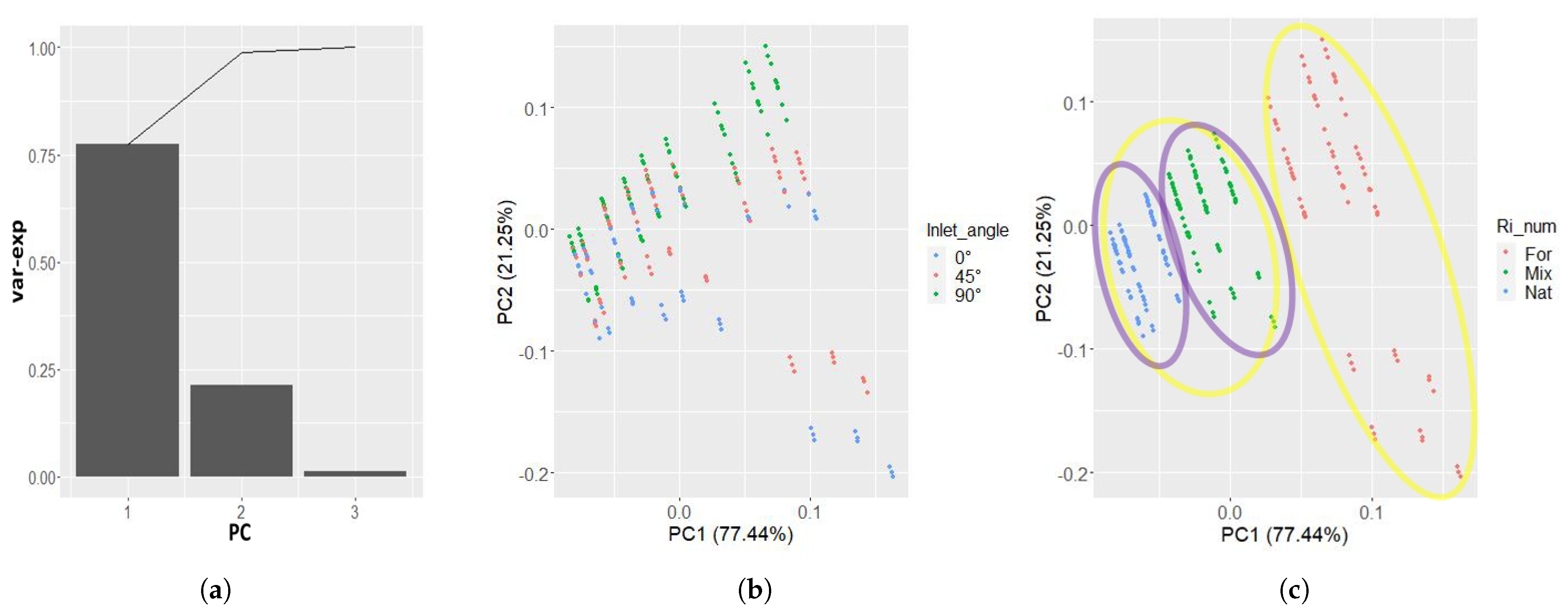
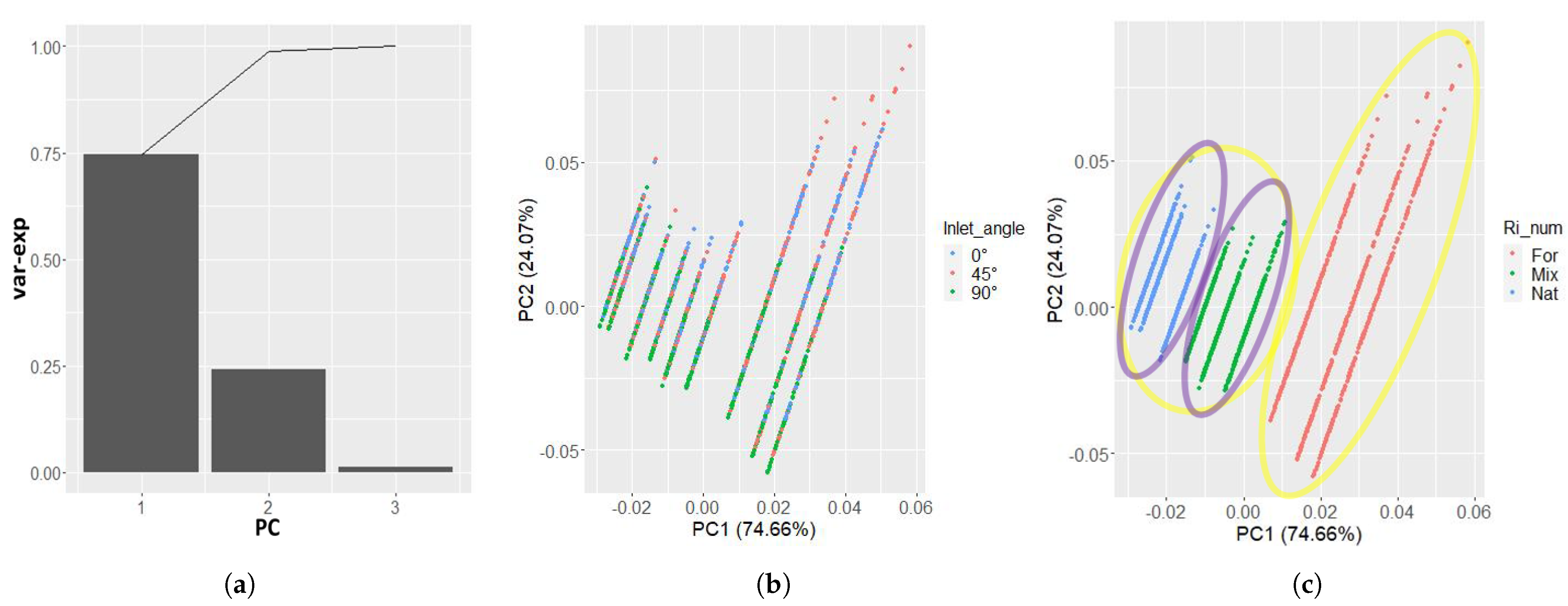
3.1. Clustering with PCA

Figure 6 summarizes the principal component analysis for the general AER. Figure 6a indicates that two principal components (PC1 and PC2) can explain almost all of the variance in the data; the third one (PC3) is insignificant. The line describes how much of the data variance is covered by all the PCs. Here, PC1 and PC2 cover almost 100% of the variance. Figure 6b,c show the projection of the data in the PCA orthogonal coordinate system, with PC1 as the x-axis and PC2 as the y-axis. As pointed out in Figure 6c by the two yellow ellipses, the points can be gathered into two main groups. However, the parameter(s) characterizing those groups were unknown. We tested out all the available parameters.

In Figure 6b, the three colors symbolize the three levels of the parameter air inlet angle ($\theta$), arbitrarily chosen to gain further understanding. It can be observed that the three levels are all mixed up in the point clouds, showing that the inlet angle is not a suitable parameter for distinguishing the point clouds. Figure 6c shows that this is not the case for the parameter Richardson number Ri. When considering this parameter, which delimits the convection type, it can be seen that the points under the natural and mixed convections (green and blue points) are two groups, forming one group, and the points corresponding to the forced convection (red points) form another group.

We repeated the PCA for the AERs of the 10 boxes’ subdivision and the results in Figure 7 present the data for all the 10 boxes. The findings for the clustering of the general AER obtained from PCA were also valid here. However, it is interesting to notice that, when comparing Figure 6b with Figure 7b (or Figure 6c with Figure 7c), the distribution of the variability between the two PCs is rather different for the general AER and the local AER (different slops). This allows us to envisage that the general AER and the local AER will have different predictable regression models.

These PCAs also confirm the second hypothesis, that flow convection type has a strong influence on the general and local AERs.

Based on those observations, we decided to split the data into the three groups—(1) natural convection (Nat), (2) mixed convection (Mix) and (3) forced convection (For)—for the subsequent analysis, to derive accurate and representative AER formulas.

3.2. AER Formulas

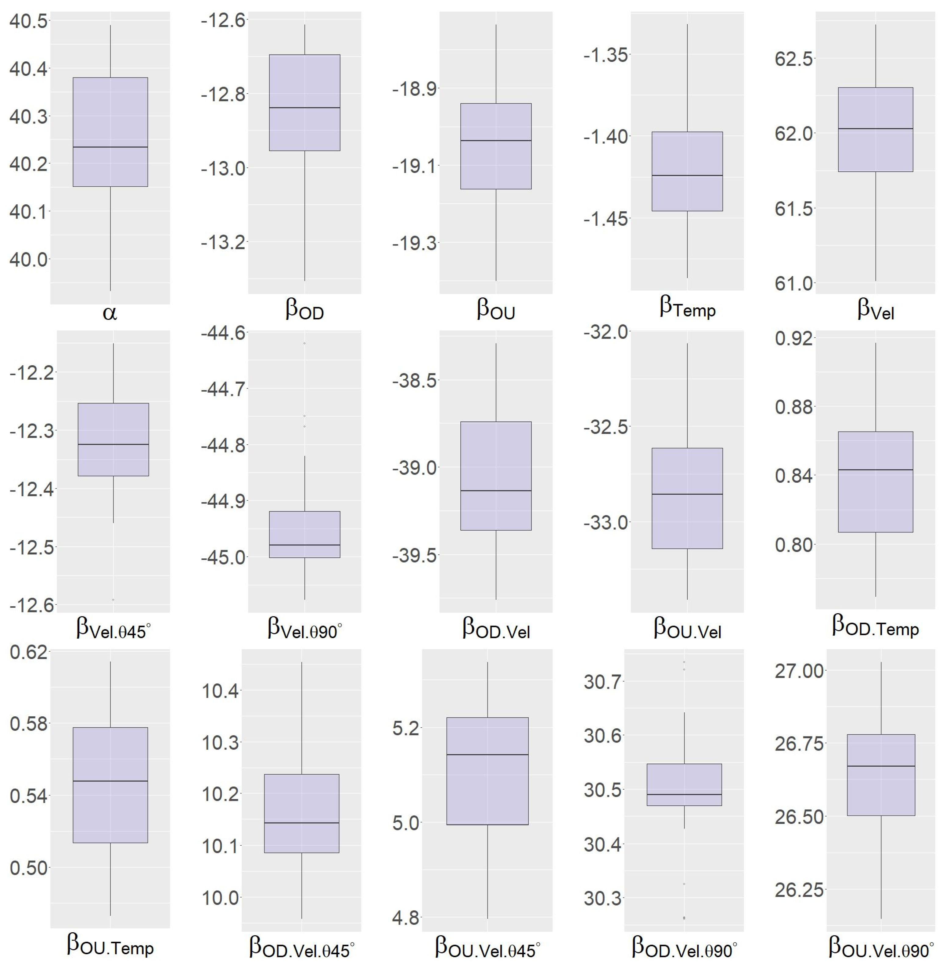
3.2.1. For the Whole Barn

Equation (9) was found by using the BIC for all the data, and then fitting the individual natural-mixed and forced groups.

Table 4. Residual standard error (RSE) and $R^2$ for all cluster groups and corresponding alphas and first part of the betas.

Cluster Group	Coefficients									RSE	${\mathit{R}}^2$
	$\mathbf{\alpha }$	${\mathbf{\beta }}_{\mathit{T}\mathit{e}\mathit{m}\mathit{p}}$	${\mathbf{\beta }}_{\mathit{V}\mathit{e}\mathit{l}}$	${\mathbf{\beta }}_{\mathit{C}\mathit{u}\mathit{r}\mathit{t}}$		${\mathbf{\beta }}_{\mathit{C}\mathit{u}\mathit{r}\mathit{t}.\mathit{V}\mathit{e}\mathit{l}}$	${\mathbf{\beta }}_{\mathit{C}\mathit{u}\mathit{r}\mathit{t}.\mathit{T}\mathit{e}\mathit{m}\mathit{p}}$	${\mathbf{\beta }}_{\mathit{V}\mathit{e}\mathit{l}.\mathit{U}}$
All	40.25	−1.42	61.98	OU	−19.06	−32.81	0.54	45$°$	−12.32	4.58	0.98
				OD	−12.85	−39.09	0.84	90$°$	−44.94
Nat-Mix	43.83	−1.01	50.87	OU	−20.25	−29.07	0.33	45$°$	−17.17	3.31	0.96
				OD	−12.85	−28.74	0.58	90$°$	−36.47
Forced	36.99	−0.76	56.92	OD	−25.86	−30.00	0.50	45$°$	−11.53	4.04	0.99
				OU	−5.06	−34.96	0.09	90$°$	−46.33

and

Table 5. Continuation of Table 4 listing the remaining betas.

Cluster Group	Coefficients
	${\mathbf{\beta }}_{\mathit{C}\mathit{u}\mathit{r}\mathit{t}.\mathit{V}\mathit{e}\mathit{l}.\mathit{U}}$
	${\mathbf{\beta }}_{\mathit{O}\mathit{U}.\mathit{U}\mathbf{45}°}$	${\mathbf{\beta }}_{\mathit{O}\mathit{U}.\mathit{U}\mathbf{90}°}$	${\mathbf{\beta }}_{\mathit{O}\mathit{D}.\mathit{U}\mathbf{45}°}$	${\mathbf{\beta }}_{\mathit{O}\mathit{D}.\mathit{U}\mathbf{90}°}$
All	5.10	26.65	10.16	30.50
Nat-Mix	10.35	22.85	11.00	20.22
Forced	4.23	27.27	10.02	32.19

show the intercepts $\alpha$ and the coefficients associated with the term of the sum (the weights ${\beta }_i$) for each groups. The $\beta$ for the curtain nonstandard cases were noted as OU for open-up and OD for open-down curtain. As expected, ${\alpha }_{all}\ne {\alpha }_{nat-mix}\ne {\alpha }_{forced}$ and ${\beta }_{i,all}\ne {\beta }_{i,nat-mix}\ne {\beta }_{i,forced}$. The resulting RSE and $R^2$ are, consequently, different, and are revealed in Table 4 as well. The readers may have noticed the small values of the coefficients ${\beta }_{Temp}$ and ${\beta }_{Curt.Temp}$. However, remember that those coefficients have to be multiplied by the temperature, with values lying between (−1 and 32). This means that their corresponding term reaches the same range as the other terms of the equation.

$$\begin{array}{cc}\hfill AER=& \alpha +{\beta }_{Curt}\times \delta \left(Curt\right)+{\beta }_{Temp}\times Temp+{\beta }_{Vel}\times Vel+{\beta }_{VelU}\times Vel\times \delta \left(\theta \right)\hfill \\ & +{\beta }_{Curt.Vel}\delta \left(Curt\right)\times Vel+{\beta }_{Curt.Temp}\delta \left(Curt\right)\times Temp\hfill \\ \hfill & +{\beta }_{Curt.Vel.U}\delta \left(Curt\right)\times Vel\times \delta \left(\theta \right)\hfill \end{array}$$

(9)

with $\delta \left(Curt\right)=\left\{\begin{array}{c}1,Curt\in \{OU,OD\}\hfill \\ 0,Curt\notin \{OU,OD\}\hfill \end{array}\right.$ and $\delta \left(\theta \right)=\left\{\begin{array}{c}1,\theta \in \{45°,90°\}\hfill \\ 0,\theta \notin \{45°,90°\}\hfill \end{array}\right.$

Looking at the extracted Equation (9), it appears that the parameter $L/W$ ratio is missing. This indicates that the ratio has no significant effect on the general AER. This is consistent with the findings of [12]. This means that the convection type added to the study does not significantly interact with the $L/W$ ratio to influence the general AER. Further comparison with [12] results means we can observe that here, too, there is notable impact from the wind speed, the wind direction, opening configuration and the interaction effects between them. This is also consistent with earlier experimental and numerical studies, which particularly highlight the importance of opening height and wind incident angle. For example, ref. [25] found, in wind tunnel experiments, a reduction in the air exchange rate of around 70% when closing half of the sidewall openings. Wind tunnel experiments reported by De Paepe et al. [26,27] indicated that the AER via the outlet opening was reduced by up to 85% when the upper 12% of the sidewall opening was closed, and it was reduced by about 40% when moving from 0$°$ to 90$°$ wind incident angle. Numerical studies by [10] indicated a reduction in the AER of around 20% when closing the lower third, and by around 35% when closing the upper third of the sidewalls. [28] even reported a reduction in the air exchange by almost 90% when only bottom part of the sidewalls was open, and a reduction of 60% when moving from a 0$°$ to 90$°$ wind incident angle, based on numerical studies. However, all of those studies considered only isothermal conditions and focused on forced convection regimes. The present work, as a novelty, investigated the role of temperature and showed that it has also a non-negligible impact.

A closer look at the coefficients lets us notice the following:

• ${\beta }_{Vel}$ multiplied with $Vel$ produced high equation values. This means that the velocity magnitude has a strong impact on the increase in the AER.
• ${\beta }_{Temp}$ is negative, showing that with increasing temperature the AER tends to decrease. This effect is slightly dampened for the reduced opening configurations (${\beta }_{Curt.Temp}$).
• Another interesting observation is that the reduction in the opening decreases the AER. ${\beta }_{Curt}$ and ${\beta }_{Curt.Vel}$ are both negative and have the same magnitude as the intercept. This goes together with the observation of [10]. In his paper, he investigated the influence of several opening configurations on the flow pattern and the airflow rate of an NVDB for high-velocity magnitude at the 0$°$ airflow direction. He also observed that the AER of the curtain Open Down is slightly less than the Open Up configuration. It is also consistent with the wind tunnel experiments of [26], who also reported a significant reduction in the AER when closing parts of the sidewall opening, where a lower air exchange was observed in the open-down case than in the open-up case. The same can be noted in our study when looking at how ${\beta }_{OD.Vel}<{\beta }_{OU.Vel}$ for the forced convection group (high velocity), which means that the higher the velocity, the more the AER is reduced for the Open Down curtain compared to the Open Up curtain. On the other hand, as ${\beta }_{OD}$ > ${\beta }_{OU}$, for lower velocities (in this setting around 1 m/s), the air exchange in the open-up and open-down cases will be nearly equal, but still considerably reduced compared with the fully open case. The latter fits well with the observations in the wind tunnel experiments of [25].
• Changing in the incoming air inlet angle also reduced the AER (${\beta }_{Vel.\theta }$ is negative). This effect is even more accentuated for 90$°$ inlet angle, since ${\beta }_{Vel.\theta 90°}$ is around three times ${\beta }_{Vel.\theta 45°}$. This is also consistent with previous reports on the effect of wind incident angle [27,28]. However, when the opening is reduced, we observed an attenuation by the positivity of ${\beta }_{Curt.Vel.\theta }$. The attenuation is not complete, since $\mid {\beta }_{Vel.\theta }\mid >\mid {\beta }_{Curt.Vel.\theta }\mid$.

Additionally, the RSE of the groups natural-mixed and forced is smaller than the RSE for the “all” group (original data group without clustering) with a corresponding AER range between 18 h${}^{-1}$ and 198 h${}^{-1}$. While all $R^2$ are very high (extremely close to the upper limit 1), the natural-mixed group has the smallest one, suggesting that the equation fits the data relatively well.

To minimize the risk of over-fitting, we further tested the robustness of Equation (9) by randomly taking 95% of the available data and fitting the corresponding coefficients. For example, if we call one test test${}_1$, we find the equation:

$$\begin{array}{cc}\hfill AER=& {\alpha }_{test1}+{\beta }_{Curt,test1}\times \delta \left(Curt\right)+{\beta }_{Temp,test1}\times Temp+{\beta }_{Vel,test1}\times Vel\hfill \\ & +{\beta }_{Vel.U,test1}\times Vel\times \delta \left(\theta \right)+{\beta }_{Curt.Vel,test1}\times \delta \left(Curt\right)\times Vel\hfill \\ & +{\beta }_{Curt.Temp,test1}\times \delta \left(Curt\right)\times Temp+{\beta }_{Curt.Vel.U,test1}\times \delta \left(Curt\right)\times Vel\times \delta \left(\theta \right)\hfill \end{array}$$

(10)

with $\delta \left(Curt\right)=\left\{\begin{array}{c}1,Curt\in \{OU,OD\}\hfill \\ 0,Curt\notin \{OU,OD\}\hfill \end{array}\right.$ and $\delta \left(\theta \right)=\left\{\begin{array}{c}1,\theta \in \{{45}^{°},90°\}\hfill \\ 0,\theta \notin \{45°,90°\}\hfill \end{array}\right.$

We tested how well the equation with those coefficients can predict the remaining 5% of the data by looking at the $R^2$ and RSE. This operation is repeated n times (in our case n = 20). We consequently obtained a series of ${\alpha }_{test.i}$ and ${\beta }_{-,test.i}$ (with $i=1...n$). To provide an idea of how much the fitted model depends on the selection of training data, we chose to plot a distribution for each coefficient as a boxplot in Figure 8 for the group “all”. The reference for each coefficient boxplot was the coefficients from the 100% data (the coefficients of Table 4, first horizontal line, group “all”). Looking at Figure 8, we observed that the individual coefficients diverge very little from their reference values. The mean $R^2$ over the 20 tests was equal to 0.984 (0.985 and 0.983) for the 95% training data and 0.975 (between 0.911 and 0.993) for the 5% test data.

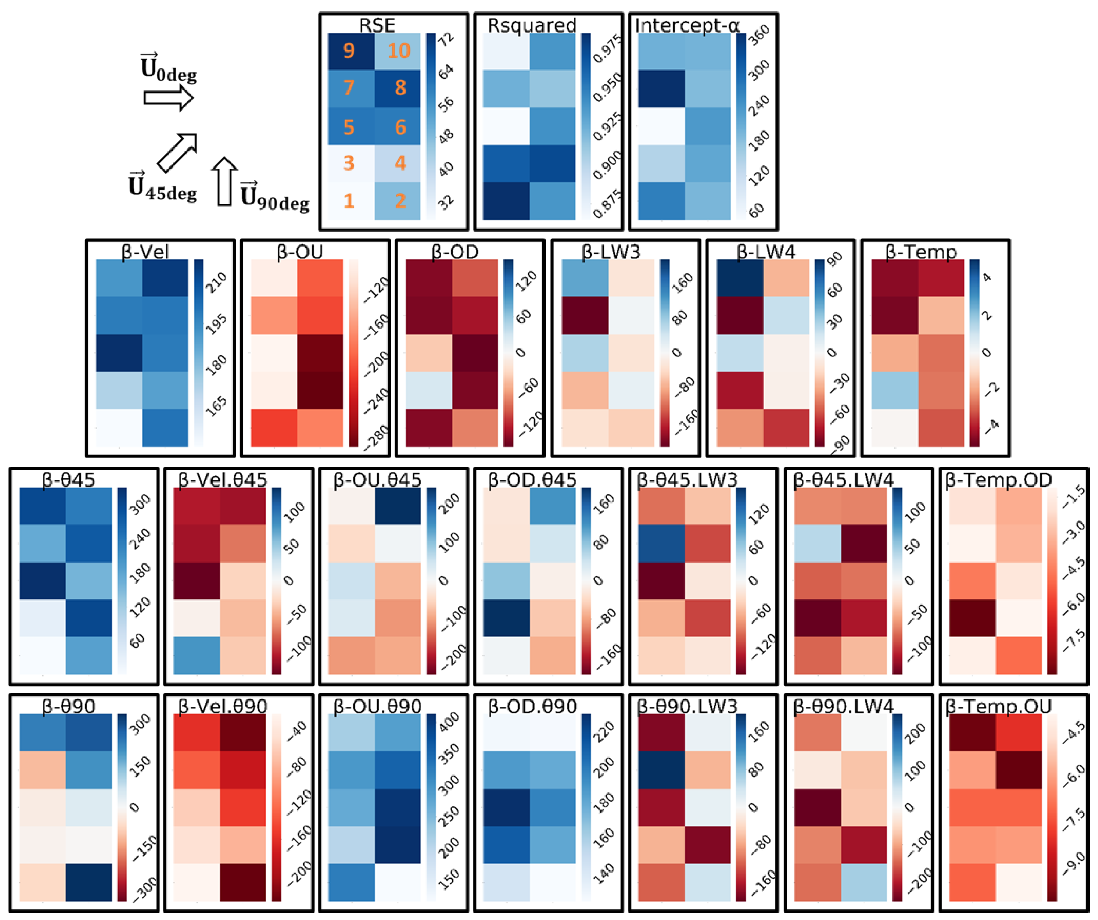
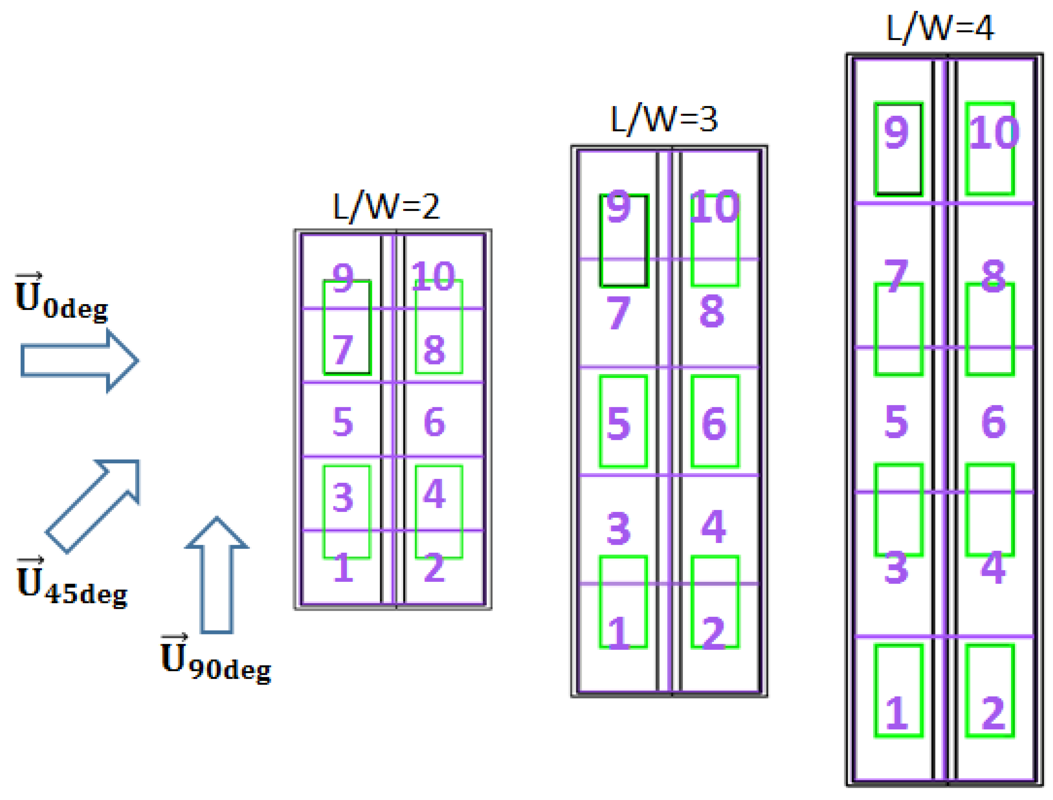
3.2.2. For the 10 Boxes Subdivision

Finding a good fitting model for all three convection groups was not possible. Here, the clustering played an importing role. As it was first formed by looking separately at each group, better results were obtained. Using the BIC as the model selection criterion, we found the following equation to best fit the data of the forced convection group in terms of $R^2$ and RSE (for an AER range theoretically between 121 h${}^{-1}$ and 1033 h${}^{-1}$):

$$\begin{array}{cc}\hfill AE{R}_{Box.i}=& {\alpha }_i+{\beta }_{Curt.i}\times \delta \left(Curt\right)+{\beta }_{\theta .i}\times \delta \left(\theta \right)+{\beta }_{L/W.i}\times \delta (L/W)+{\beta }_{Temp.i}\times Temp\hfill \\ & +{\beta }_{Vel.i}\times Vel+{\beta }_{Vel.\theta .i}\times Vel\times \delta \left(\theta \right)+{\beta }_{Curt.Temp.i}\times \delta \left(Curt\right)\times Temp\hfill \\ & +{\beta }_{Curt.\theta .i}\times \delta \left(Curt\right)\times \delta \left(\theta \right)+{\beta }_{L/W.\theta .i}\times \delta (L/W)\times \delta \left(\theta \right)\hfill \end{array}$$

(11)

with

$$\delta \left(Curt\right)=\left\{\begin{array}{c}1,Curt\in \{OU,OD\}\hfill \\ 0,Curt\notin \{OU,OD\}\hfill \end{array}\right.;$$

$$\delta \left(\theta \right)=\left\{\begin{array}{c}1,\theta \in \{45°,90°\}\hfill \\ 0,\theta \notin \{45°,90°\}\hfill \end{array}\right.;$$

$$\delta (L/W)=\left\{\begin{array}{c}1,L/W\in \{3,4\}\hfill \\ 0,L/W\notin \{3,4\}\hfill \end{array}\right.$$

Equation (11) should be seen as a prediction of the AER of one individual box i (with $i=1...10$, see Section 2.4 for the subdivision on the barn into ten equal volumes, called boxes). Each box i possesses its own values for the coefficients $\alpha$ and ${\beta }_k$. There are ten equations with the same independent variables (in red and green) but with location-specific coefficients $\alpha$ and ${\beta }_k$. There are some similarities when comparing Equation (11) to Equation (9). Five of the nine terms are identical (the ones in green), demonstrating that there is a relationship between the general AER and the local AERs. However, these are not completely the same, since the variable $L/W$ appears twice. This leads to the conclusion that, for local AERs, $L/W$ cannot be ignored, thus validating our choice to use this parameter in the analysis even if previous studies concluded that it was irrelevant.

It is worth noting that the average of the $R^2$ over the ten boxes is equal to 0.93 (between 0.86 and 0.98), which is lower than the 0.98 for the Equation (9) on the general AER, but still translates to a good fit with the data. All $R^2$ and RSE values, as well as the coefficients ${\alpha }_i$ and ${\beta }_{ki}$ for the boxes are summarized in Figure 9. The chosen color code is dark blue—white—dark red to easily distinguish the variation between the boxes. When, for a single coefficient, all box-values are positive, the minimum value is associated with the white color and the maximum value with dark-blue. For the opposite case, when all box-values are negative, the maximum value is associated with white and the minimum with the dark-red. Finally, for the case when the box-values are both positive and negative, dark-blue was assigned to the maximum, white to zero and dark-red to the minimum. The following points summarize the conversations on the influence of each parameter on the individual boxes:

• As in the general AER, the velocity magnitude (${\beta }_{Vel}$ at the beginning of the second row) has a strong effect on the increase in the $AE{R}_{box.i}$. However, for the inlet angle $\theta$ is 45$°$(${\beta }_{Vel.\theta 45}$), the effect is attenuated, especially at the upper half of the barn (boxes 5–10). For $\theta$ = 90$°$ (${\beta }_{Vel.\theta 90}$) the AER${}_{box.i}$ are decreased even more, but this time for the boxes of the rear half of the barn (boxes 2, 4, 6, 8, 10). We noted that the pattern of ${\beta }_{\theta 45}$ is approximately complementary to ${\beta }_{Vel.\theta 45}$ and also ${\beta }_{\theta 90}$ to ${\beta }_{Vel.\theta 90}$: such a contrast slightly dampens the effect of ${\beta }_{Vel.\theta -}$. This is consistent with contemporary knowledge of the indoor air flow pattern of naturally ventilated cattle buildings. For example, [29] concluded, from on-farm measurements in the AOZ with 25$°$ and 70$°$ incident wind angle, that the speed and direction of the incident wind significantly influence the air velocity in the AOZ.
• Here, the temperature (${\beta }_{Temp}$) decreases the $AE{R}_{box.i}$ (except at boxes 1 and 3), but the effect is more pronounced in the rear and upper half of the barn (boxes 2, 4, 6, 7, 8, 9, 10). This effect is the same for the reduced openings; see the last column, ${\beta }_{Temp.OD}$ and ${\beta }_{Temp.OU}$.
• The similarity with the general AER continues. The coefficients for the curtain levels Open Down and Open Up (${\beta }_{OD}$, ${\beta }_{OU}$, second row) are both negative, meaning that the reduced opening size reduces the local AER (OU more than OD, with stronger effects at the rear half of the barn). This goes together with the indoor air flow pattern observed by [17] wind tunnel experiments with different opening configurations. The study reported a slightly lower wind speed in the AOZ in the Open Down case compared to the open case and a considerably lower wind speed in the AOZ in the Open Up case compared to the Open case. While, in our study, the reduction effect on the local AER was generally stronger in the rear half of the barn, the changes in the air flow pattern reported by [17] were more pronounced in the front part of the barn. However, this difference might be explained by the fact that [17] considered only one cross-section through the building and a model with a L/W ratio of nearly 1:1.
• ${\beta }_{OD.\theta 45}$, ${\beta }_{OU.\theta 45}$, ${\beta }_{OD.\theta 90}$ and ${\beta }_{OU.\theta 90}$ (third and fourth columns from the left) allowed us to analyze the influence of inlet angle $\theta$ on the reduced opening configurations. We note that with increasing inlet angle, the coefficients also increase. For 45$°$, the boxes 2, 4, 6 of the rear half and 7, 9 of front half are still negative, while their counterparts on the other side are positive. For 90$°$, they all turn positive, with high values complementary to the original coefficient ${\beta }_{OD}$ and ${\beta }_{OU}$. (Where there are high values of ${\beta }_{OD.\theta 90}$, we have low values of ${\beta }_{OD}$. The same applies to ${\beta }_{OU.\theta 90}$ and ${\beta }_{OU}$.)
• Patterns for ${\beta }_{LW3}$ and ${\beta }_{LW4}$ can hardly be recognized. However, we noticed that the values switch from positive to negative (or high to low) from a box of one half-barn side (front or rear) to the other half-barn side, except for box 1 and 2, which have almost same values. An average over all the boxes gave a value near to zero. This might explain why the $L/W$ parameter has no significant impact on the general AER, since the local AERs compensate for each other.
• When $L/W$ interacts with the inlet angle $\theta$ (second and third columns from the right), we note that the patterns of ${\beta }_{\theta -.LW3}$ are complementary to ${\beta }_{LW3}$, and the ones of ${\beta }_{\theta -.LW4}$ to ${\beta }_{LW4}$. However, the magnitude of the ${\beta }_{\theta -.LW-}$ is higher than the magnitude of the ${\beta }_{LW-}$, especially for ${\beta }_{\theta 90.LW-}$. This means that for a higher $L/W$, increasing the inlet angle tends to create an opposite effect to that for smaller $L/W$.

Equation (12) represents the fitted model for $AE{R}_{Box.i}$ of the mixed convection group. Again, the green-colored terms are the ones that can be found in Equation (9) of the general AER. The underlined terms correspond to the terms matching with Equation (11). Here, we note that both equations are more similar to $curt\times L/W$ than $curt\times temp$.

$$\begin{array}{cc}\hfill AE{R}_{Box.i}=& {\alpha }_i+{\beta }_{Curt.i}\times \delta \left(Curt\right)+{\beta }_{\theta .i}\times \delta \left(\theta \right)+{\beta }_{L/W.i}\times \delta (L/W)+{\beta }_{Temp.i}\times Temp\hfill \\ & +{\beta }_{Vel.i}\times Vel+{\beta }_{Vel.\theta .i}\times Vel\times \delta \left(\theta \right)+{\beta }_{Curt.\theta .i}\times \delta \left(Curt\right)\times \delta \left(\theta \right)\hfill \\ & +{\beta }_{L/W.\theta .i}\times \delta (L/W)\times \delta \left(\theta \right)+{\beta }_{Curt.L/W.i}\times \delta \left(Curt\right)\times \delta (L/W)\hfill \end{array}$$

(12)

with

$$\delta \left(Curt\right)=\left\{\begin{array}{c}1,Curt\in \{OU,OD\}\hfill \\ 0,Curt\notin \{OU,OD\}\hfill \end{array}\right.;$$

$$\delta \left(\theta \right)=\left\{\begin{array}{c}1,\theta \in \{45°,90°\}\hfill \\ 0,\theta \notin \{45°,90°\}\hfill \end{array}\right.;$$

$$\delta (L/W)=\left\{\begin{array}{c}1,L/W\in \{3,4\}\hfill \\ 0,L/W\notin \{3,4\}\hfill \end{array}\right.$$

Analyzing the coefficients of the Equation (12) summarized in Figure 10, we can extract the following information:

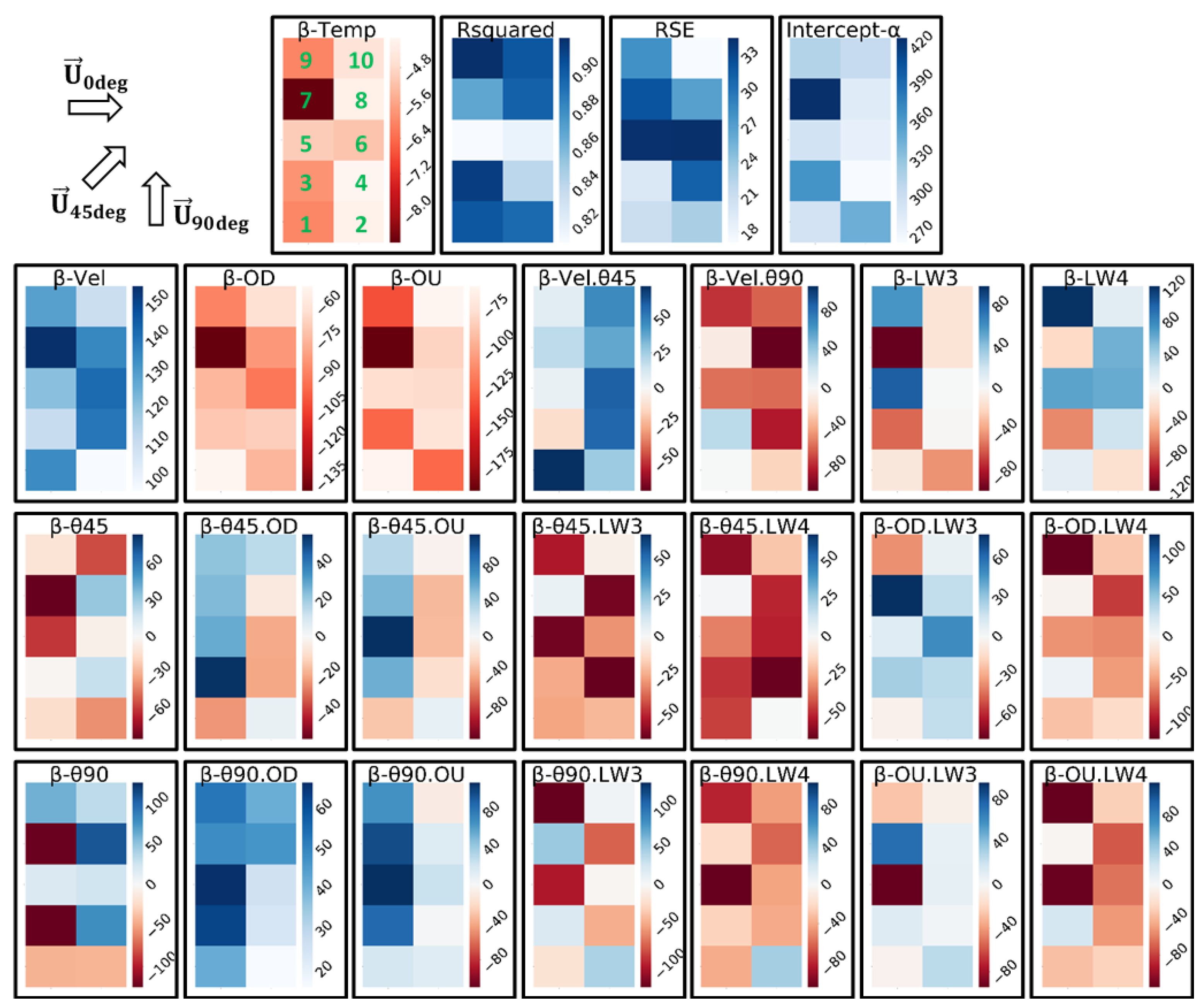
• Again, as for the general AER, the velocity magnitude (${\beta }_{Vel}$ at the beginning of the second row) has a significant effect on the increase in the $AE{R}_{box.i}$. However, for the inlet angle $\theta$ 45$°$ (${\beta }_{Vel.\theta 45}$) the effect is attenuate. For $\theta$ = 90$°$ (${\beta }_{Vel.\theta 90}$), $AE{R}_{box.i}$ are decreased, especially for the boxes of the rear half of the barn (boxes 2, 4, 6, 8, 10).
• Here, too, the temperature decreases the $AE{R}_{box.i}$ but the effect is more pronounced in the front half of the barn (boxes 1, 3, 5, 7, 9).
• The coefficients for curtain levels Open Down and Open Up (${\beta }_{OD}$, ${\beta }_{OU}$, second row) are both negative, meaning that the reducing opening size reduces local AER (OD reduces more in the front half of the barn, except for box 1, with a pattern that is complementary to alpha).
• For ${\beta }_{OD.\theta 45}$, ${\beta }_{OU.\theta 45}$, ${\beta }_{OD.\theta 90}$ and ${\beta }_{OU.\theta 90}$ (second and third columns from the left), we note that with increasing inlet angle, the coefficients also increase. For 45$°$, the boxes at the rear half of the barn (and for box 1), the coefficients are still negative, but for 90$°$, they all turn positive. However, the lowest values are retained for the boxes in the rear half of the boxes and box 1.
• As in the forced convection case, the values of ${\beta }_{LW3}$ and ${\beta }_{LW4}$ vary between high and low from one half of the barn to the other. When the openings are reduced (${\beta }_{Curt.LW-}$), there are small changes in most of the boxes (light colors which means close to zero). The three boxes with high values (5, 7, 9) are complementary to their respective original ${\beta }_{LW-}$.

Here, the mean $R^2$ over the 10 boxes is about 0.875 (between 0.81 and 0.92), which is lower than that for the forced convection group but still acceptable. The mean RSE is about 26 (minimum of 17 and maximum of 34), while the $AE{R}_{Box}$ range is between 151 h${}^{-1}$ and 530 h${}^{-1}$.

Unfortunately, we could not find a fitting equation for the natural convection with an acceptable $R^2$ and RSE. We tried a logarithmic transformation, but it was still not satisfactory. This means that the local AER prediction for natural convection does not follow a linear “rule” with respect to the chosen independent parameter. Further investigations are needed to explore other possibilities.

4. Conclusions

In the present work, the prediction of the general and local AER of NVDBs based on five independent parameters was investigated using the statistical method general linear model. In comparison to previous works, here, the temperature was added as an influencing parameter, leading to consideration of the three different flow convection types. We first found that the AER dataset for both the general and local cases could be clustered into three groups, which perfectly correspond to the convection types. This confirms the second hypothesis stated in the introduction, regarding the importance of the temperature–velocity interaction for the AER.

Furthermore, an equation modelling the general barn AER with high accuracy ($R^2$ = 0.98) was found, which was in agreement with previous studies. Our study confirmed that the barn’s length-to-width ratio ($L/W$) did not have a significant influence on the general AER and that reducing the opening size reduces the AER. In addition, we observed that, with increasing inlet angle ($\theta$), the latter effect was dampened. This scenario could also be seen for the local AER. The velocity magnitude ($Vel$) had a significant impact on the general and local AER, while the temperature tended to decrease the AER. Interactions between the considered parameters were also noted to influence the AER.

This present work also investigated the AER locally, in the form of ten equal volume subdivions (called box). It was noted that the only possibility of finding a reliable modelling was by considering each convection group separately. The equations for the forced and mixed convection groups indicated a similar behavior to the general group. Nevertheless, at the same time, this behavior is more complex. This time, $L/W$ has a non-negligent impact on the AER${}_{Box}$, in such a way that the positive and negative box-coefficients associated with this parameter compensate for themselves. This could explain the absent $L/W$ for the general AER model. We also noticed some patterns where, depending on the equation term, the front half of the barn was more strongly affected than the rear half of the barn, or vice-versa. These findings allow us to confirm the first hypothesis, that the local AERs have a different behavior depending on their position and relative to the general AER. While it was possible to extract modelling equations for the forced and mixed groups, it was hard to find a representative model for the natural convection group.

This leaves exciting expectations for future works. For example, a non-linear model of the natural convection group could be explored. In addition, a more precise subdivision could be investigated: for example, 40 boxes instead of 10. Another possible direction could be the implementation of position coordinates in the modelling of a local AER equation.

References

- Grethe, H.; Christen, O.; Balmann, A.; Bauhus, J.; Birner, R.; Bokelmann, W.; Gauly, M.; Knierim, U.; Latacz-Lohmann, U.; Nieberg, H.; et al. Wege zu Einer Gesellschaftlich Akzeptierten Nutztierhaltung. Ber. Landwirtsch. Z. Agrarpolit. Landwirtsch. 2015, 221, 1–171. [Google Scholar] [CrossRef]
- Beattie, V.; O’Connell, N.; Kilpatrick, D.; Moss, B. Influence of environmental enrichment on welfare-related behavioural and physiological parameters in growing pigs. Anim. Sci. 2000, 70, 443–450. [Google Scholar] [CrossRef]
- Umweltschutztechnik, F. Emissionen und Immissionen aus Tierhaltungsanlagen—Haltungsverfahren und Emissionen000Schweine, Rinder, Geflügel, Pferde; VDI/DIN: Berlin, Germany, 2011; p. 84. [Google Scholar]
- Samer, M.; Fiedler, M.; Müller, H.J.; Gläser, M.; Ammon, C.; Berg, W.; Sanftleben, P.; Brunsch, R. Winter measurements of air exchange rates using tracer gas technique and quantification of gaseous emissions from a naturally ventilated dairy barn. Appl. Eng. Agric. 2011, 27, 1015–1025. [Google Scholar] [CrossRef]
- Norton, T.; Sun, D.W.; Grant, J.; Fallon, R.; Dodd, V. Applications of computational fluid dynamics (CFD) in the modelling and design of ventilation systems in the agricultural industry: A review. Bioresour. Technol. 2007, 98, 2386–2414. [Google Scholar] [CrossRef]
- Bartzanas, T.; Boulard, T.; Kittas, C. Numerical simulation of the airflow and temperature patterns in a greenhouse equipped with insect-proof screen in the openings. Comput. Electron. Agric. 2002, 34, 207–221. [Google Scholar] [CrossRef]
- Ferziger, J.H.; Peric, M. Computational Methods for Fluid Dynamics, 3rd ed.; Springer: Berlin/Heidelberg, Germany, 2002; p. 364. [Google Scholar] [CrossRef]
- Bartzanas, T.; Kacira, M.; Zhu, H.; Karmakar, S.; Tamimi, E.; Katsoulas, N.; Lee, I.B.; Kittas, C. Computational fluid dynamics applications to improve crop production systems. Comput. Electron. Agric. 2013, 93, 151–167. [Google Scholar] [CrossRef]
- Lee, I.; Bitog, J.P.; Hong, S.W.; Seo, I.; Kwon, K.; Bartzanas, T.; Kacira, M. The past, present and future of CFD for agro-environmental applications. Comput. Electron. Agric. 2013, 93, 168–183. [Google Scholar] [CrossRef]
- Saha, C.K.; Yi, Q.; Janke, D.; Hempel, S.; Amon, B.; Amon, T. Opening Size Effects on Airflow Pattern and Airflow Rate of a Naturally Ventilated Dairy Building—A CFD Study. Appl. Sci. 2020, 10, 6054. [Google Scholar] [CrossRef]
- Doumbia, M.; Hempel, S.; Janke, D.; Amon, T. Prediction of the Local Air Exchange Rate in Animal Occupied Zones of a Naturally Ventilated Barn. In Proceedings of the Sustainable Decisions in Bio-Economy (CIOSTA 2019)—XXXVIII CIOSTA & CIGR V International Conference, Rhodes, Greece, 24–26 June 2019; pp. 29–34. [Google Scholar]
- Yi, Q.; Zhang, G.; Amon, B.; Hempel, S.; Janke, D.; Saha, C.; Amon, T. Modelling air change rate of naturally ventilated dairy buildings using response surface methodology and numerical simulation. Build. Simul. 2020, 14, 827–839. [Google Scholar] [CrossRef]
- Doumbia, E.M.; Janke, D.; Yi, Q.; Amon, T.; Kriegel, M.; Hempel, S. CFD modelling of an animal occupied zone using an anisotropic porous medium model with velocity depended resistance parameters. Comput. Electron. Agric. 2021, 181, 105950. [Google Scholar] [CrossRef]
- Janke, D.; Caiazzo, A.; Ahmed, N.; Alia, N.; Knoth, O.; Moreau, B.; Wilbrandt, U.; Willink, D.; Amon, T.; John, V. On the feasibility of using open source solvers for the simulation of a turbulent air flow in a dairy barn. Comput. Electron. Agric. 2020, 175, 105546. [Google Scholar] [CrossRef]
- Blocken, B. LES over RANS in building simulation for outdoor and indoor applications: A foregone conclusion? Build. Simul. 2018, 11, 1–50. [Google Scholar] [CrossRef] [Green Version]
- Betriebe Milchkuhhaltung nach Bestandsgrößenklassen. Ergebnisse der repräsentativen Agrarberichterstattung (Vorläufig). 1993.
- Yi, Q.; König, M.; Janke, D.; Hempel, S.; Zhang, G.; Amon, B.; Amon, T. Wind tunnel investigations of sidewall opening effects on indoor airflows of a cross-ventilated dairy building. Energy Build. 2018, 175, 163–172. [Google Scholar] [CrossRef]
- Gebremedhin, K.; Wu, B. Simulation of flow field of a ventilated and occupied animal space with different inlet and outlet conditions. J. Therm. Biol. 2005, 30, 343–353. [Google Scholar] [CrossRef]
- Saha, C.; Fiedler, M.; Ammon, C.; Berg, W.; Loebsin, C.; Amon, B.; Amon, T. Uncertainty in calculating air exchange rate of naturally ventilated dairy building based on point concentrations. Environ. Eng. Manag. J. 2014, 13, 2349–2355. [Google Scholar] [CrossRef]
- Marek, R.; Nitsche, K. Praxis der Wärmeübertragung Grundlagen—Anwendungen—Übungsaufgaben, 4., neu bearbeitete auflage ed.; Carl Hanser Verlag GmbH & Co. KG: Munich, Germany, 2015; p. 343. [Google Scholar]
- Wang, X.; Zhang, G.; Choi, C.Y. Evaluation of a precision air-supply system in naturally ventilated freestall dairy barns. Biosyst. Eng. 2018, 175, 1–15. [Google Scholar] [CrossRef]
- Saha, C.; Fiedler, A.; Amon, T.; Berg, W.; Amon, B.; Brunsch, R. Assessing effects of different opening combinations on airflow pattern and air exchange rate of a naturally ventilated dairy building—A CFD approach. In Proceedings of the International Conference of Agricultural Engineering AgEng, Zurich, Switzerland, 6–10 July 2014. [Google Scholar]
- Mondaca, M.R.; Choi, C.Y. Assessment of Dairy Cow Geometries in Computational Modeling. In Proceedings of the 2015 ASABE Annual International Meeting, Chicago, IL, USA, 3–5 May 2015. [Google Scholar]
- Dalgaard, P. Introductory Statistics with R, 2nd ed.; Springer Science & Business Media: Berlin/Heidelberg, Germany, 2008; p. 364. [Google Scholar]
- Shen, X.; Su, R.; Ntinas, G.K.; Zhang, G. Influence of sidewall openings on air change rate and airflow conditions inside and outside low-rise naturally ventilated buildings. Energy Build. 2016, 130, 453–464. [Google Scholar] [CrossRef]
- Paepe, M.D.; Pieters, J.G.; Cornelis, W.M.; Gabriels, D.; Merci, B.; Demeyer, P. Airflow measurements in and around scale model cattle barns in a wind tunnel: Effect of ventilation opening height. Biosyst. Eng. 2012, 113, 22–32. [Google Scholar] [CrossRef]
- Paepe, M.D.; Pieters, J.G.; Cornelis, W.M.; Gabriels, D.; Merci, B.; Demeyer, P. Airflow measurements in and around scale-model cattle barns in a wind tunnel: Effect of wind incidence angle. Biosyst. Eng. 2013, 115, 211–219. [Google Scholar] [CrossRef]
- Rong, L.; Liu, D.; Pedersen, E.; Zhang, G. The effect of wind speed and direction and surrounding maize on hybrid ventilation in a dairy cow building in Denmark. Energy Build. 2015, 86, 25–34. [Google Scholar] [CrossRef]
- Fiedler, M.; Berg, W.; Ammon, C.; Loebsin, C.; Sanftleben, P.; Samer, M.; von Bobrutzki, K.; Kiwan, A.; Saha, C.K. Air velocity measurements using ultrasonic anemometers in the animal zone of a naturally ventilated dairy barn. Biosyst. Eng. 2013, 116, 276–285. [Google Scholar] [CrossRef]