Article

Estimating Pesticide Inputs and Yield Outputs of Conventional and Organic Agricultural Systems in Europe under Climate Change

Research Unit Sustainability and Global Change, Department of Earth Sciences, Universität Hamburg, Grindelberg 5, 20144 Hamburg, Germany
Agronomy 2021, 11(7), 1300; https://doi.org/10.3390/agronomy11071300
Submission received: 27 May 2021 / Revised: 23 June 2021 / Accepted: 24 June 2021 / Published: 26 June 2021
(This article belongs to the Special Issue Agriculture and Crop Protection: Relationship with Climate Change)

Abstract

:
Simulating organic agriculture is a considerable challenge. One reason is that few models are capable of simulating crop-pest interactions and the yield losses they cause. Here, a recently developed process-based crop-pest model (Pest-EPIC) was used to simulate conventional and organic agriculture in the European Union for the years 1995–2100. Yields and pesticide application rates were calibrated against FAOSTAT and Eurostat data. Results indicate that current pesticide application rates may be sufficient to control pests and diseases even at the end of the century. The range of simulated yield differences under organic and conventional agriculture under current conditions (e.g., wheat 21–55% (mean 34%) lower yields; potatoes 20–99% (mean 56%) lower yields) closely matched recorded values. Under climate change, the gap between yields under conventional and organic management will remain constant for some crops (e.g., at 3 t/ha for potatoes), but others—susceptible to a larger number of pests and diseases—may experience a widening of the yield gap (e.g., increase of yield difference from 0.8 to 1.6 t/ha for wheat). The presented results-dataset may in future be a valuable resource for integrated assessments of agricultural land use and policy planning, but the inherent uncertainty is still very high.

1. Introduction

Pesticides are an integral part of modern agriculture and are used to control diseases, increase crop yields, and support food preservation [1]. Pesticides in combination with mineral fertilizers enabled modern intensive agriculture, thus mitigating the trend towards agricultural area expansion [2] and slowing down the import rates of virtual agricultural land by countries with high demand for agricultural goods [3]. However, only a small proportion of the pesticides applied to crops actually reaches their target. The rest enters into the environment, contaminating air, water, and soil, and often persists over long time periods [4,5]. Due to concerns about these negative impacts, policy-makers started to outlaw many pesticides and tightened regulations, while consumers began to buy food produced without pesticides. One consequence is that the area under organic agriculture continues to increase. It currently amounts to 71.5 million hectares globally, roughly 1.5% of the total arable area [6]. Regional environmental impacts of this trend are largely positive and include a higher biodiversity [7] and a higher soil organic carbon and nitrogen content [8]. Yields, however, are 15–50% lower in organic systems than in conventional ones [9,10,11,12], which may cause higher rates of agricultural area expansion and/or larger imports of virtual agricultural land, shifting more intensive agriculture towards other regions. This concern is especially pressing considering the high amount of food waste, the continuous global population, and income growth, as well as the rising demand for animal proteins and bioenergy products, which will most likely necessitate a significant increase in agricultural area in the coming decades [13,14].
Considering these complex interactions and the additional challenge climate change will pose in many regions, it is more important than ever for policy-makers, scientists, and stakeholders to be able to draw on multiple tools and datasets to inform their decisions and direct their actions and resources. One such resource is robust information on per-hectare production capacities under different management systems and their environmental impacts [15], in this case conventional and organic agricultural systems. Data on past yields have been collected for many years by national governments and international organizations such as the FAO, and a variety of models is available to estimate yields under future climatic conditions and different levels of water and nutrient availability [15]. However, quantifying the impacts of pests and diseases, a prerequisite for simulating organic agriculture, has remained a challenge [16,17]. The immense variety of pathogens and pests, their complex interactions with target crops, and their often unknown response to changes in climate have prompted scientists to mainly focus on developing models for short-term, tactical questions, applicable for specific climates and/or locations and specific pest-crop systems [16,18,19]. Only recently have models been developed that explicitly focus on simulating crop-pest interactions for entire agricultural systems at larger scales (e.g., [20]). This paper presents the first attempt to use such a model to simulate simplified representations of conventional and organic agriculture at multi-national level.
The study has multiple goals. The first is to assess if the currently available data on pesticide application rates in the EU are sufficient to calibrate the model in such a way that yield quantities, as well as pesticide application rates, can be simulated adequately. The second goal is to use the calibrated model to study if the simulated quantity of pesticide application rates in conventional agricultural systems of the EU will change over the course of the 21st century. Application rates in the model are dependent on the damage level caused by pests and diseases, and the literature thus far is inconclusive about how climate change will affect pest pressure as a whole [21,22,23,24,25]. The third goal is to simulate a simplified version of organic agriculture, inspect the simulated current yield levels for plausibility, and continue to project expectant yields for the next decades. The reported range of yield gaps between organic and conventional agricultural systems is large [9,10,11,12], and it is uncertain how it will develop under climate change. The last goal is to assess the capability of the model to simulate soil property changes under the different management options. Organic agriculture is not only viewed positively because organic produce is less contaminated by pesticides [26], but also because soil quality in organic systems tends to be higher [8,27]. If a dataset such as the one presented in this paper should be used in the future for integrated assessments of land use options, the effects of the different management strategies on soil properties should also be depicted accurately.

2. Material and Methods

2.1. Pest-EPIC Model

All simulations were run with the Pest-EPIC model (for details, see Rasche and Taylor [20]). The model is based on EPIC v0810 [28,29], a biogeophysical model of crop growth on one homogeneous field. Original submodels of EPIC v0810 include hydrology, soil nutrient dynamics, wind and water erosion, plant environment control, tillage, and crop growth, all driven by daily weather data (minimum and maximum temperature, solar radiation, precipitation, relative humidity and wind speed). For Pest-EPIC, additional submodels for the simulation of fungal diseases, insect pests and weed infestations were added. In the weed submodel, the number of seeds in the seed bank is tracked and weeds are grown depending on these seeds and germination rates. The weeds compete with the crop for light, water and nutrients. A herbicide may be applied manually in the operation file, or an application may be triggered if the weed LAI (leaf area index) surpasses a user-specified ratio to crop LAI. In the insect submodel, a biological temperature response function is used to model the daily feeding rate, from which population growth is derived. Mortality is dependent on temperature and nutrient availability. Optimal temperature, mortality at 0 °C, body mass and main feeding/damage target (aboveground biomass, root biomass, leaf area or radiation use efficiency) are pest-specific. Crop stress is dependent on the feeding rate, which may trigger an insecticide application if a user-defined threshold is exceeded. Insecticide applications may also be scheduled by the user. In the disease submodel, disease spread depends on coefficients of primary and secondary infection, abundance of spores and host density. The number of spores increases depending on a humidity and temperature function, and decreases according to a decay rate. Optimal temperature and humidity, decay rate and the coefficients of infection are pest specific. Crop stress is dependent on the ratio of healthy to infected plant tissue, which may compromise radiation use efficiency or the different biomass compartments. If the stress-factor exceeds a user-defined threshold, a fungicide application may be triggered, or an application can be scheduled by the user.
Prior to the simulations, the Pest-EPIC model was improved from the version described in Rasche and Taylor [20]. In the old version, all crops were grouped in one of the following crop groups: warm or cold season annual legumes, perennial legumes, warm or cold season annuals, perennials, evergreen or deciduous trees, cotton or N-fixing trees. This is a feature of EPIC v0810, which allows adjustments to the growth functions depending on the growth type. We used these groups to define “host” groups, meaning that crops from the same group serve as hosts to the same diseases and should not be grown in rotation. This solution was not satisfactory and was addressed now by adding a new crop parameter denoting a specific “host group” to which a crop belongs. The new host groups are: (1) all cereals except corn, (2) cotton, (3) corn, (4) oil seeds (rape, sunflower, oil flax, soybeans), (5) potatoes, (6) sugar beet, (7) other, (8) weeds.

2.2. Data

Most of the input data for the running of the model (Table 1) were taken from a database originally compiled for the CCTAME project (https://cordis.europa.eu/project/id/212535 (last accessed on 26 June 2021)). The derivation procedure for the simulation units was described in detail in Balkovič, et al. [30], the datasets in UNIBA [31]. The simulated area covers the area currently used for crop production in the EU (approximately 1,084,087 km2), divided into 38,738 simulation units located in 16 countries (details on the number of simulation units in each country, the irrigated area, the fertilization rates, and the crops grown can be found in Table S1 of the Supplementary Materials). For the presentation of aggregated simulation results, yield and pesticide values of every crop grown on a single simulation unit were weighted by the frequency of the crop in the rotation; the weight of the results of the single simulation units was determined by the area they cover in each country. Daily climate data for the years 1995 to 2100 were provided in bias-corrected form by the Climate Service Center for Germany (GERICS), and covers projections based on relative concentration pathway (RCP) scenarios 2p6, 4p5, and 8p5 (optimistic, intermediate, and worst-case scenario, respectively). Data on pesticide use in the different EU member states were taken from an Eurostat report about the use of plant protection products in the EU in the years 1992–2003 [32]. The values are listed in Table S2 of the Supplementary Materials. The year 2003 was chosen as the reference year because it was the only one for which the application rates of different pesticide types were reported, not only the sum of all pesticides. A more recent usable dataset was not available, as the one published in October 2020 by Eurostat (aei_pestuse) was still missing data for many crops, years and/or EU-countries (such as France and Germany).

2.3. Scenarios and Simulation Settings
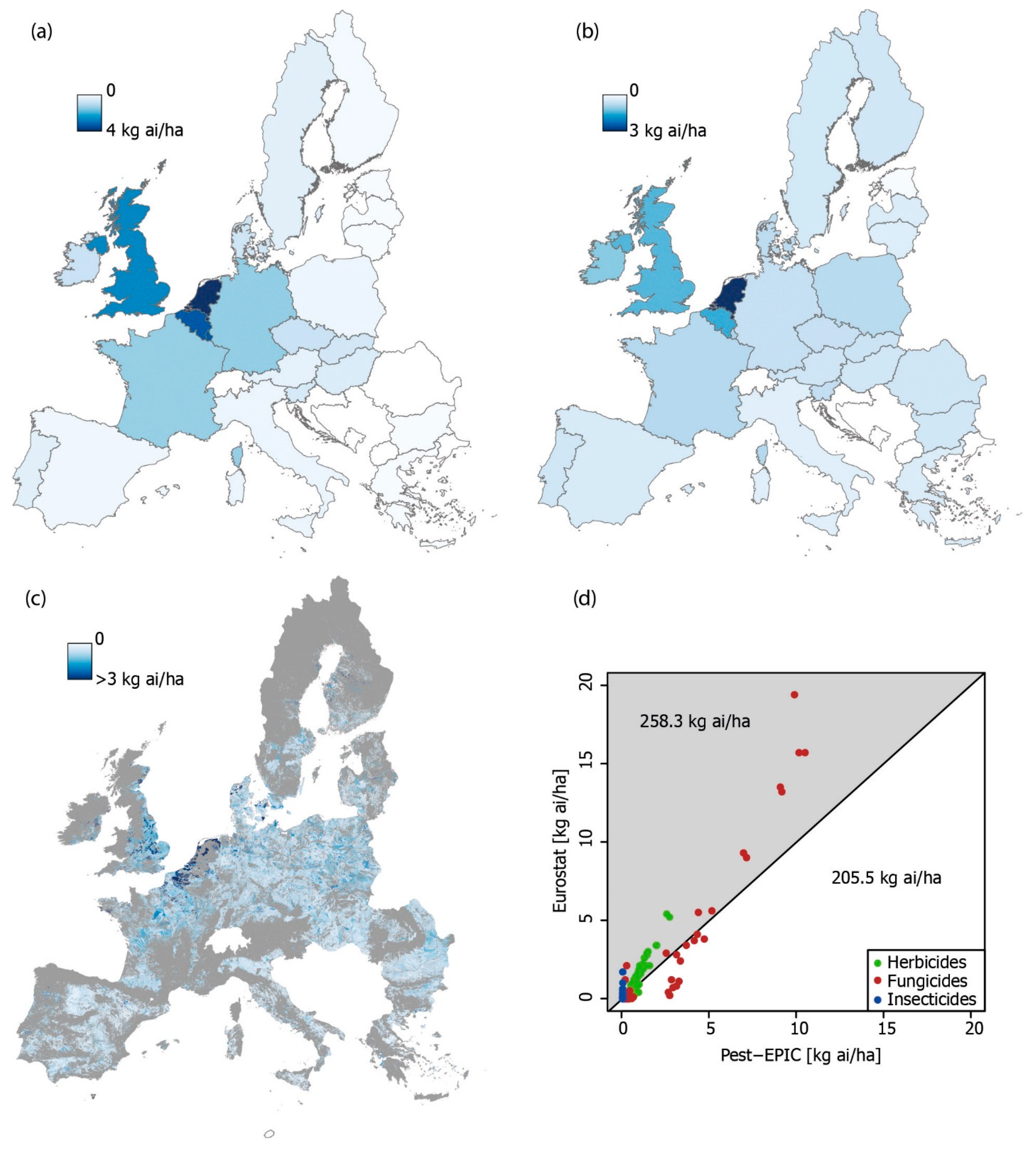
In the conventional scenario, herbicide applications were simulated as follows: half of the reported herbicide application rate for the single crops was applied as a pre-emergent herbicide before planting, which was scheduled manually in the operation file (cf. Table S2). For the duration of the growing season, no more herbicide applications were scheduled, but further applications were allowed if the stress-threshold was reached. The same setting was applied to fungicide applications, but pre-emergent applications were only scheduled for potatoes. Irrigation was simulated as recorded in the CCTAME database based on the agricultural statistics and land cover data, with one exception: rice crops were always irrigated. Fertilization with nitrogen, phosphorous and potassium fertilizers was also simulated as recorded in the CCTAME database (cf. Table S1), as was the crop rotation for the single simulation units. In the organic scenario, manure was applied instead of elemental N/P/K fertilizers. The application rate was adapted to the nitrogen content of the manure but capped at a maximum of 250 kg/ha. No pesticides were applied, and the crop rotation was adapted to include a legume catch crop for N-fixation and green manure fertilization if the field was fallow for more than 60 days between two crops. Since only the presence of pesticides, the fertilizer type, and the legume catch crop is different between the simulated conventional and organic management systems, the simulated organic system should be considered a simplified version of actual organic systems. Usually, the crop rotation used in organic systems is different, intercropping is practiced, compost may be added to the soil in addition to green manure, the tillage is different, and biopesticides may be applied instead of conventional pesticide products. Since these practices are not uniform across farms and, in some cases, difficult to model, the differences between organic and conventional farming were reduced to the most important drivers for the simulations.
The initial settings for the pest submodel were adapted from Rasche and Taylor [20]. For weeds, a seed bank initial value of 500 seeds/m2, a seed half-life of 1000 days, a 100 seed weight of 303 mg and a germination rate (%) of 0.5 was assumed. The variables describing the various pest-insects and diseases are listed in Table S3 of the Supplementary Materials. A short sensitivity analysis of the input variables is provided there as well. It should be kept in mind that even if the different parameter sets are named after specific diseases and insect pests, they should be considered more as an amalgam of all pests with similar characteristics (climatic envelopes, targets, damage rates), and not as exact representations of this one disease/pest. The probability of occurrence (Table S4 of the Supplementary Materials) was used to adapt the importance of each disease/pest amalgam for each host group. Herbicide applications were triggered when weed LAI reached 20% of crop LAI, but only executed every 20 days, and in the manufacturer recommended dosage. A fungicide application was triggered once 10% of the leaf surface shows lesions; and an insecticide application was triggered if the damage rate (biomass consumed by insects) surpassed 10%. Fungicides may be applied every 10 days, insecticides every 7 days in manufacturer recommended doses.

2.4. Calibration

Crop yields and pesticide application rates were calibrated simultaneously prior to the scenario runs. The calibration of yields is generally straightforward, as reported crop-specific yields are usually available, there is only one yield-value per crop, and simulated yields are directly influenced by a variety of crop parameters which can be adapted if necessary. Pesticide application rates, on the other hand, are not generally available, much less at crop level, there are a variety of pesticides which are applied under different circumstances, and pesticide application rates in themselves serve only as a proxy for the underlying pest-pressure, which should be calibrated instead. The only available dataset on pesticide use in the European Union contains pesticide application rates per (aggregated) crop group, consisting of cereals, maize, oil seeds, potatoes, sugar beet, and other [32]. Application rates for the different pesticide types used on the different crop groups are only available for the year 2003, and only for the top-five chemical classes applied. Pesticides like growth regulators or molluscicides are not considered in Pest-EPIC and had to be deleted from the top-five list. This left few data points in some cases (see Table S1 of the Supplementary Materials). For a quality check of the dataset, the reported rates were compared to values from a dataset covering the UK for the year 2003 [34]. The rates differ widely in most cases (Table 2), indicating a considerable bias in (presumably) the Eurostat data, but for a lack of alternatives at the EU-level, the Eurostat-dataset was used for calibration regardless.
The calibration simulations were run for the years 1985 to 2005 to provide a spin-up period and generate enough data-points to cover at least one whole rotation on every simulation unit. It was then checked if simulated and reported yields and the total amount of pesticides were comparable at the country level. If not, crop parameters, the probability of occurrence of pests (Table S4 of the Supplementary Materials), and/or the pesticide application trigger were adapted. The calibration of yields was checked visually for every crop grown in every country and deemed satisfactory if the range of simulated yields over the years 1985 to 2005 was in proximity to the range of reported yields for the same time-period for a majority of crops (Figure S1 of the Supplementary Materials).
The calibration of pesticide application rates was checked visually and numerically, but due to the missing crop-specific values and general uncertainty of the reported data, it was difficult to decide when to call the calibration successful. The decision was made to focus on the total application rate, not single pesticide types, and to try to recreate the relative intensity of application rates between countries rather than absolute values. The reasoning was that (i) it is likely that the relative differences between countries are more accurate than the absolute values in the Eurostat dataset, and (ii) in practice, pesticide application rates are generally higher than would be necessary to treat a disease or infestation, which is not the case in Pest-EPIC. With this calibration setup, it was possible to establish a baseline, and calculate the change relative to the presumed baseline under different management scenarios and future time-periods.
Figure 1a,b show reported and simulated pesticide application rates in the different EU member states. The spatial patterns do not agree perfectly, but closely. To give an impression of the bias inherent in aggregating to country-level, Figure 1c was added, which shows simulated total pesticide application rates on the single simulation units. Here, mean values for pesticide application rates can surpass 6 kg ai/ha (ai: active ingredient) on single units. Even though the focus was on the sum of all pesticides applied, the application rates of the three different pesticide types were nevertheless checked to ensure that pest pressure from the different pest types was adequately simulated (Figure 1d). Reported application rates were on average higher than simulated ones, with a sum of 258.6 kg ai/ha reported and 205.5 simulated (sums of all data-points, each representing one crop group in one country). The calibration could have been continued to more closely match reported data. However, considering the overall high uncertainty inherent in the calibration data, the lack of crop-specific data, and the fact that the pest-calibration was a calibration by proxy (pesticide application rates as an indicator for pest pressure), the quality of the calibration was deemed acceptable.

3. Results

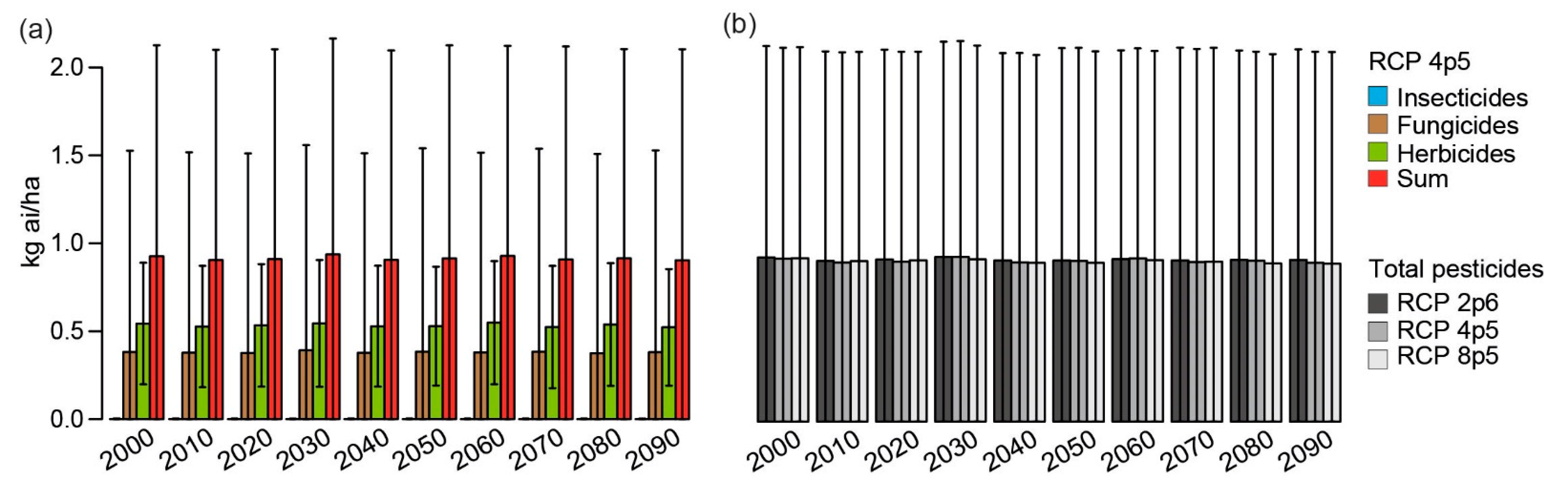
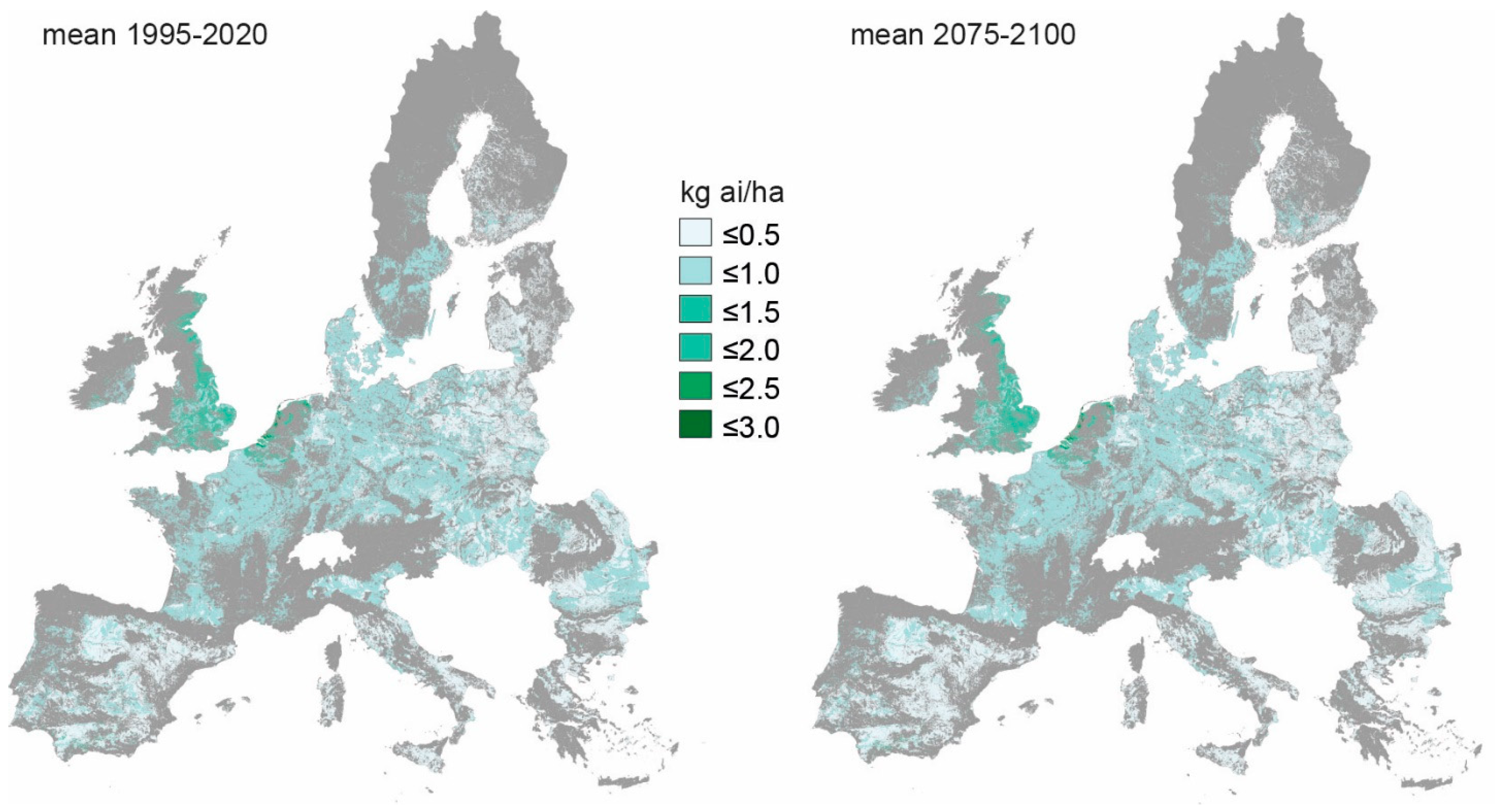
3.1. Will Pesticide Application Rates Change in the Next Decades Due to Higher Pest Pressure?

Mean pesticide application rates as well as the range of application rates in the European Union will not change significantly in the coming decades, according to the simulation results. This applies to the single pesticide types—insecticides, fungicides, and herbicides—as well as the sum (Figure 2a), and can be observed over all three climate scenarios (Figure 2b). Even at the crop-specific level, pesticide application rates only change significantly for two crops, sunflowers and cotton, where application rates experience a very slight decrease of 0.001 kg ai/ha per decade (not shown). This finding may be initially surprising, but can be explained by the simulation setup. Every pest has a single, fixed probability of occurrence for every crop pest group. If, based on this probability, an infestation or infection is initialized on a field in a specific growing season, the stress-triggered pesticide application mechanism ensures that the pest is adequately managed in the current growing season; and the crop rotation prescribed for most of the fields prohibits an accumulation of pathogens that may exacerbate pest damages when the crop is next grown. Since the simulated application rates do not change over time, we can conclude that current pesticide application rates in combination with currently observed crop rotations are sufficient to ensure crop protection even in the future, although pathogens and pest insects with higher optimal temperatures for propagation do benefit from climate change in the simulations. The result could also indicate that current pesticide application rates are rather too high relative to pest population dynamics, and that the surplus is sufficient for controlling future disease/pest levels.
It would have been possible that even though pesticide application rates stay constant over time at EU-level, the spatial distribution of rates in the EU member states changes. This is not the case; the spatial pattern of herbicide application rates remains almost unchanged from the baseline to the future (Figure 3). The same can be observed for the spatial patterns of insecticide and fungicide application rates (not shown).

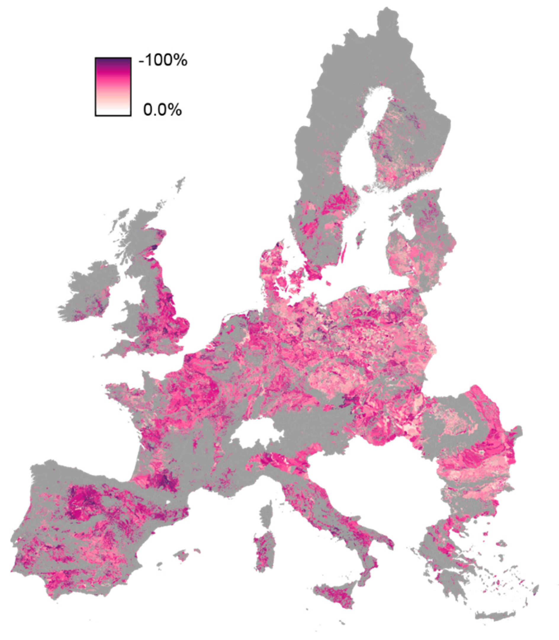
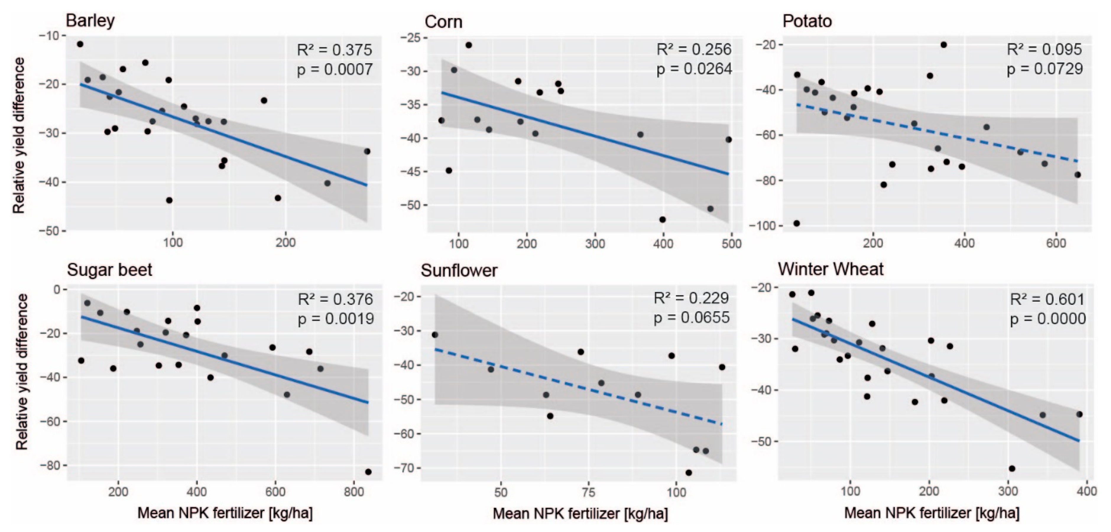
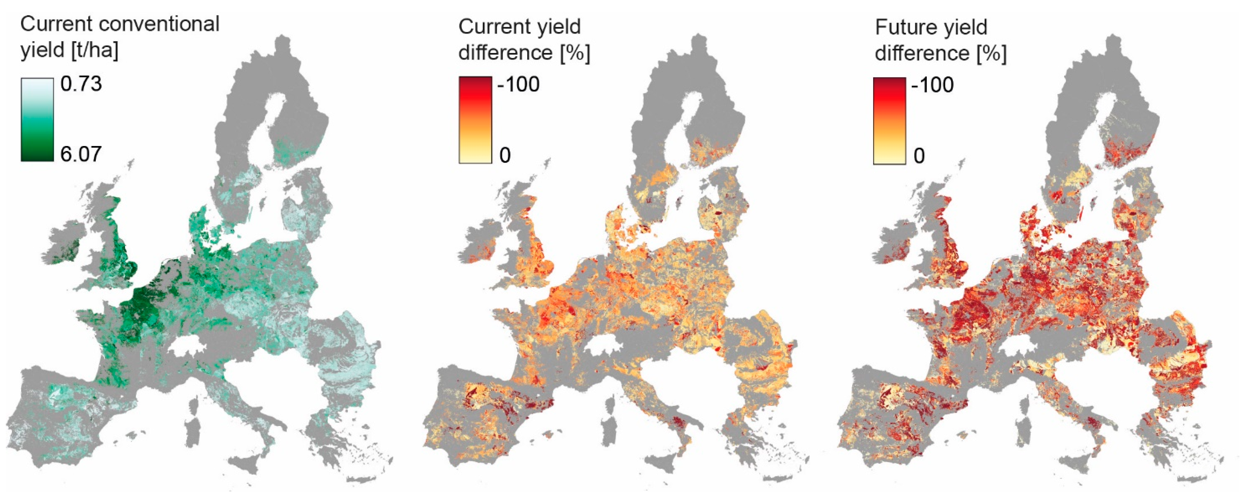
3.2. How Large Is the Simulated Yield Gap between Conventional Agriculture and Organic Agriculture in Europe?

The average relative difference between all yields simulated in the conventional scenario (always used as the baseline) and yields simulated in the organic scenario in the years 1995 to 2020 is −60.5% (±15.2%). There is no clear geographic pattern to the intensity of the loss, but it appears that losses are slightly lower in the Eastern half of Europe (Figure 4). The result should be interpreted with caution, however, since the yields of different crops can differ widely in terms of tons per hectare, and the share of each crop changes from simulation unit to simulation unit, which may lead to exaggerated relative differences if the mean yield on a single simulation unit was very low to begin with, and decreased further. If single countries and crops are considered, and the results of the single simulation units weighted according to the area, the relative differences between yields in the conventional scenario and yields simulated in the organic scenario are more nuanced (Table 3). In the case of current winter wheat yields, for example, the relative differences between the yields simulated in the conventional and the organic scenario range from −55.3% in Ireland to −21.1% in Portugal, with an average of −33.7%. In the case of potato yields, the range is much wider, with a maximum difference of −99.0% in Estonia, a minimum difference of −20.1% in Ireland, and an average difference of −55.6%. The least differences between yields were simulated for field peas, where the mean change is −10.9%, with the highest change in Italy (−27.2%), and the lowest in Sweden (−1.9%).
To explain the magnitude of the differences between yields produced under conventional and organic agriculture in the different countries, mean elevation, mean annual temperature, precipitation sum, relative humidity and solar radiation, mean ratio of irrigated area, and mean NPK-fertilizer amount were used as explanatory variables. Linear models were fitted for each crop separately, and non-significant variables were excluded in order of their significance rating and relative importance. It was not possible to find significant models for peas, potatoes, rapeseed, and winter rye. For barley, the model with the highest explanatory power (R2 adj. = 0.37) included only NPK-fertilizer. For corn, the model included mean annual temperature, relative humidity, solar radiation, and NPK-fertilizer (R2 adj. = 0.55). For sugar beet, the model contained NPK-fertilizer, and mean precipitation sum (R2 adj. = 0.52). For sunflower, the model included NPK-fertilizer, and mean annual relative humidity (R2 adj. = 0.53), and for winter wheat, the model contained only NPK-fertilizer (R2 adj. = 0.60). The results show that while climate variables do influence the yield gap, the amount of fertilizer plays a dominant role, with higher amounts of fertilization leading to a larger relative difference in conventional and organic yields. This could also be shown for corn, potato, sugar beet, and sunflower, when models containing only NPK-fertilizer as the explanatory variable were fitted to the data (Figure 5).

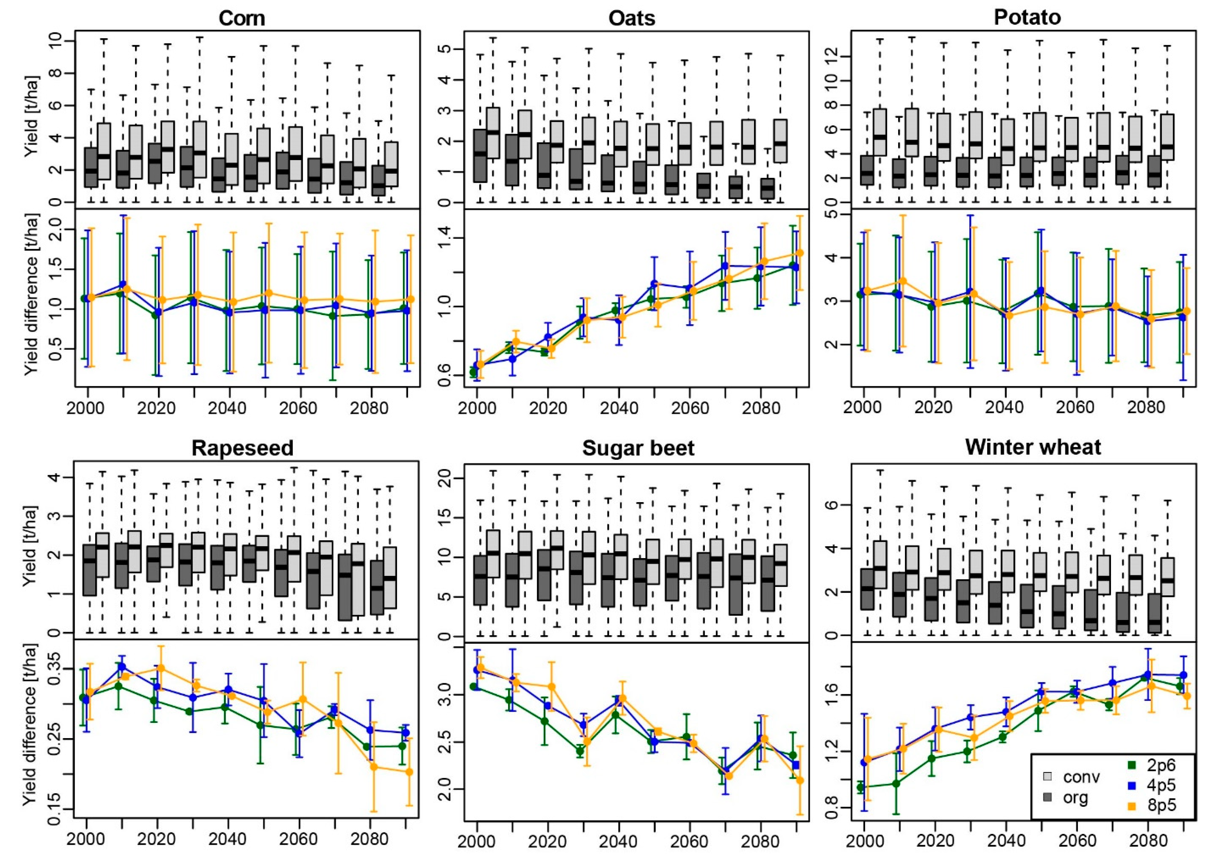
3.3. Will the Yield Gap Change under Climate Change?

The progression of yield differences between conventional and organic agriculture until 2100 is crop-specific and differs in trend. In the climate scenario RCP 4p5, there was no significant change simulated for corn and corn silage; a significant increase in yield differences for barley, oats, rice, winter rye, and winter wheat; and a significant decrease for peas, potatoes, rapeseed, sugar beet, and sunflowers (Figure 6, not all shown).
The increase in yield differences is more pronounced than the decrease, with increases of 0.6–1.0 t/ha and decreases of 0.05–0.15 t/ha (except sugar beet, where the decrease is ~1 t/ha). One explanation for these differing trends is that the crops belong to the different pest response groups: corn/corn silage (no change), cereals (yield gap increase), and potatoes/sugar beets/oil seeds (decrease). ‘Cereals’ comprise the crops barley, durum wheat, oats, rice, winter rye, and winter wheat, and it follows that the group is susceptible to more diseases than the ‘corn’ group, just because it consists of six crops instead of only two (corn, corn silage). This means that the probability of occurrence for a single fungal disease is low, but the number of potential diseases with a low probability of occurrence is high in the ‘cereal’ group. The opposite applies to potatoes, sugar beet, and oil seeds, which have high probabilities of occurrence for a few fungal diseases. The results show that this leads to a higher disease pressure over time for cereals, because more diseases occur on the field by chance, and a relatively constant pressure for potatoes, sugar beet, and oil seeds, where diseases spread from the beginning but no new diseases occur over time. When looking at the example of winter wheat, the spatial distribution of yield differences under conventional and organic agriculture does not follow a clear pattern (Figure 7). In the period 1995–2020, very large differences in average yields can be observed in Northern Spain, Southern Italy, small parts of Eastern France and Northern Austria, and several other small regions across Europe. In the period 2075–2100, the differences in wheat yields are almost uniformly high in all regions of Europe, indicating that the combined effects of climate change and pest pressure affect wheat production under the two different systems in all countries almost equally.

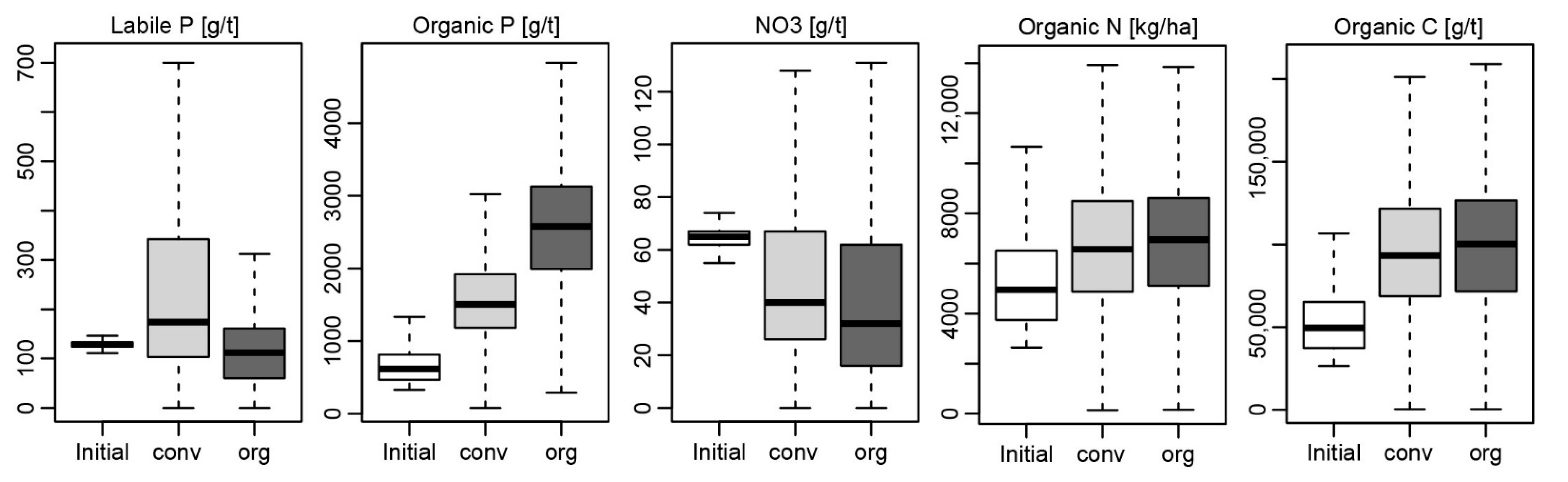
3.4. How do Soil Nutrient Values Respond to the Different Cultivation Methods?

All simulations started with the same initial soil data. At the end of the simulation period in 2100, organic soil phosphorus and nitrogen values were significantly higher in the organic scenario than in the conventional scenario (Figure 8), with a higher increase for phosphorus (mean values increased by 60–79%, depending on RCP scenario), than for nitrogen (2–8%). Conversely, values of mineral phosphorus and nitrogen decreased significantly under organic agriculture (by 47–59% and 19–35%, respectively). Organic carbon contents of the soil increased minimally but still significantly from the conventional to the organic scenario (4–8%). The results show that the model recreates expected patterns of changes in soil nutrient availability: Manure and green manure applications under organic agriculture enrich soil organic matter and the nutrient fraction bound in organic compounds, whereas mineral fertilizers applied in conventional agriculture (conventional scenario) supply the soil with a higher amount of nutrients in forms that are more readily available for plant uptake.

4. Discussion

This study represents the first attempt to use a process-based crop-pest model to simulate a simplified representation of conventional and organic agricultural systems at a large scale. Results of studies like this not only offer insights into potential changes in agricultural inputs and outputs under climate change, they are also a useful resource for integrated assessments of land use and management changes in the agricultural sector, especially when observed datasets may become unreliable as reference points under the progressing climatic changes [16]. Based on the simulation results, current pesticide application rates should be adequate to control pests, diseases and weeds even at the end of the century. It has been documented in the literature that a variety of crop pests and pathogens move northwards (cf. [25,35]), which would mean that pest pressure should increase in Europe, at least in the northern countries. Since the spread of infection and the insect feeding rates have a temperature-dependent component in the model, Pest-EPIC is in theory capable of recreating this trend. However, no increase in pesticide application rates can be observed in the simulation results. It would seem that either the temperature sensitivity is too low in the model—relative humidity is the more critical factor for diseases and the model is more sensitive to it—or current pesticide application rates include a prophylactic quantity that is sufficient to control future levels of disease. The literature is also still inconclusive about the net-effects of climate change on pest pressure. Soil moisture, for example, may increase the severity of diseases affecting the belowground biomass of plants if near the saturation point [36], whereas dry conditions may stress plants and lower their resistance to infections [37], but also reduce the buildup of migratory pest-insect species [38]. Some insects, such as mites, favor hot and dry conditions, whereas wingless species may disappear under the same conditions due to lack of food [24]. The effect of elevated CO2 levels is equally inconclusive [39,40]. It is, therefore, possible that the results are accurate and that the net-effect of climate change on pest damage is so small that current pesticide application rates suffice for its control. This conclusion only applies to situations where no new pests are introduced to the system, which was not covered by the model. However, even then, results may still be similar, as the spread of pathogens due to climate change is also highly variable, with some areas projected to have lower disease risks in the future and others higher [35,41].
Under organic management, where no pesticides are applied, the average simulated decrease in yields ranges from 11% to 56%. The range of yield losses due to pests, diseases and weeds reported in the literature is wider, and covers values from 7% to 80% [42,43,44,45], but in these studies, all agricultural systems were considered. Reports pertaining specifically to organic systems list yields as, on average, 19% lower [10], 25% lower [9], 20–45% lower [11], and 30–50% lower [12], which covers the simulated range to a high degree. These differences not only depend on pesticide applications, but also on other factors such as site characteristics, crop, and management. Oil seed crop yields e.g., may only decrease by 11% under organic management, whereas cereal yields may decrease by 26%; and average yields may decrease by 13% if best organic practices are used, whereas they decrease by 34% if the organic and conventional system are most comparable [9]. The abundance of soil-pathogens causing root and foot rots may be smaller on organic fields, and lower nitrogen concentrations in foliar tissues, often found in organic systems, may attenuate attacks by sucking pests or airborne diseases [46]. The overabundance of nitrogen in itself may increase pest occurrences [47,48], e.g., by promoting growth and prolonging the vegetative period, thereby increasing the susceptibility to diseases [36]. Leitch and Jenkins [49] found that Septoria diseases caused a potential yield loss of 5% for each 100 kg N/ha that was applied, and Veresoglou, et al. [50] showed in a meta-study that combined N and P fertilization caused a significant increase in disease severity and suggested that a surplus of nitrogen may cause pathogens to become more aggressive due to C-limitations. The presented simulation results confirm a significant relationship between yield gap size and NPK-fertilizer application rates.
Related to nutrient availability and input is soil organic matter. Soil organic carbon contents are 0–70% higher under organic farming practices [8]—in the simulations, they are on average 4–8% higher—which can influence pest pressure. A higher organic matter content can lead to higher microbial activity and thus more competition for soil-dwelling pests, but also larger amounts of CO2 releases, which is toxic to some pathogens in high concentrations [36]. Soil nitrogen contents may be 21–47% higher in organic systems, whereas plant-available phosphorous and potassium may not be influenced [8]. The simulation results differ in this regard, as organic and mineral phosphorous fractions did change significantly from one management system to the other, whereas nitrogen pools showed a low variability, but this can be an effect of the tillage system and the applied fertilizer types and amounts.

5. Conclusions

The considerable overlap between reported and simulated yield differences under organic and conventional agriculture suggests that the model is reasonably accurate in the simulation of pest damages. The results confirm the wide range in yield differences between organic and conventional systems, even under the tightly controlled boundaries of a simulation and not actual field conditions. Even though simulated pesticide application rates stay almost constant over time, the simulations under the organic management scenario indicate that pest pressure can increase if a crop is susceptible to a large number of pests and diseases. Crop yields are affected equally by climate change under organic and conventional management.
What currently limits the explanatory power of the presented data is the considerable uncertainty associated with the available data on pest pressure and pesticide use by farmers, as well as the model functions and assumptions. For example, the accuracy of the Eurostat pesticide use data does not seem to be very high, based on the comparison of pesticide-use data presented in Table 2. Since the pesticide use values of the model were calibrated to these data, the accuracy of the absolute simulated values cannot be higher, which is why the focus lies on the change over time. Further, the pest damage simulated for organic systems is likely overestimated, since it is currently not possible to simulate alternative ways of pest control in the model. The disease and insect modules are generic, meaning that all disease and insect pest dynamics are simulated using the same functions with disease/insect-specific variables. The coefficients describing the spread of a disease could not be derived from existing literature and were thus not calibrated or changed between diseases. The pesticide efficacy is based on studies collected in the EPA ECOTOX database [51] and needed to be derived for some species from similar ones, since pesticide manufacturers rarely publish their efficacy data, only toxicity studies for unrelated species.
Many of these issues could be addressed with additional, better and more readily accessible data, and further model development, but it will take substantial time and effort by many people to achieve this. Efforts are under way, Eurostat for example, plans to increase the quality of pesticide-related data by harmonizing data collection and specifying a common reference year, report format, crop selection, and aggregation level [52]. There are also many additional factors that could not be considered in this study, either due to missing data, non-existent or insufficient methods, or for being beyond the scope. These include the impact of crop breeding on yields in organic and conventional systems, the evolutionary potential of pests and diseases, potential synergies between crops and beneficial arthropods/fungi in organic systems, and possible adaptation strategies to climatic change. Until more data and knowledge is available and methods and models have been refined or newly developed, the current results should be interpreted with caution and under due consideration of all assumptions, uncertainties, and limitations.

Supplementary Materials

The following are available online at https://www.mdpi.com/article/10.3390/agronomy11071300/s1, Table S1: Aggregate characteristics of the simulation units in each country, Table S2: Use of plant protection products in 2003 in the EU member states based on Eurostat data, Table S3: Pest submodel parameters describing the different diseases and insect pests; sensitivity analysis, Table S4: Annual probability of occurrence of each pest/disease for each host group. Figure S1: Simulated (after calibration) and reported (FAOSTAT) yield distributions by country and crop.

Funding

This research was funded by the German ministry of education and research (BMBF) within the research program NorthWesternPaths, grant number FKZ 01LS1910A, and by the Deutsche Forschungsgemeinschaft (DFG, German Research Foundation) under Germany‘s Excellence Strategy–EXC 2037 ’CLICCS-Climate, Climatic Change, and Society’–Project Number: 390683824, contributing to the Center for Earth System Research and Sustainability (CEN) of Universität Hamburg.

Data Availability Statement

The data presented in this study are available in the open-access research data repository of Universität Hamburg at http://doi.org/10.25592/uhhfdm.9213.

Acknowledgments

The author wants to thank RAJ Taylor for his comments on the manuscript.

Conflicts of Interest

The author declares no conflict of interest.

References

  1. Cooper, J.; Dobson, H. The benefits of pesticides to mankind and the environment. Crop. Prot. 2007, 26, 1337–1348. [Google Scholar] [CrossRef]
  2. Waterfield, G.; Zilberman, D. Pest Management in Food Systems: An Economic Perspective. Annu. Rev. Environ. Resour. 2012, 37, 223–245. [Google Scholar] [CrossRef]
  3. Von Witzke, H.; Noleppa, S. EU Agricultural Production and Trade: Can More Efficiency Prevent Increasing ‘Land-Grabbing’ outside of Europe? Humboldt Universität zu Berlin: Berlin, Germany, 2010. [Google Scholar]
  4. Pimentel, D. Environmental and economic costs of the application of pesticides primarily in the United States. Environ. Dev. Sustain. 2005, 7, 229–252. [Google Scholar] [CrossRef]
  5. van der Werf, H.M.G. Assessing the impact of pesticides on the environment. Agric. Ecosyst. Environ. 1996, 60, 81–96. [Google Scholar] [CrossRef]
  6. Willer, H.; Schlatter, B.; Trávníček, J.; Kemper, L.; Lernoud, J. (Eds.) The World of Organic Agriculture. Statistics and Emerging Trends 2020; Research Institute of Organic Agriculture (FiBL): Frick, Switzerland; IFOAM—Organics International: Bonn, Germany, 2020; p. 337. [Google Scholar]
  7. Letourneau, D.; van Bruggen, A. Crop protection in organic agriculture. In Organic Agriculture: A Global Perspective; Kristiansen, P., Taji, A., Reganold, J.P., Eds.; CSIRO Publishing: Collingwood, ON, Canada, 2006; pp. 93–122. [Google Scholar]
  8. Erhart, E.; Hartl, W. Soil Protection through Organic Farming: A Review. Org. Farming Pest. Control. Remediat. Soil Pollut. 2009, 1, 203–226. [Google Scholar] [CrossRef]
  9. Seufert, V.; Ramankutty, N.; Foley, J.A. Comparing the yields of organic and conventional agriculture. Nature 2012, 485, 229–232. [Google Scholar] [CrossRef]
  10. Ponisio, L.C.; M’Gonigle, L.K.; Mace, K.C.; Palomino, J.; de Valpine, P.; Kremen, C. Diversification practices reduce organic to conventional yield gap. Proc. R. Soc. B-Biol. Sci. 2015, 282. [Google Scholar] [CrossRef] [Green Version]
  11. Halberg, N.; Sulser, T.B.; Høgh-Jensen, H.; Rosegrant, M.W.; Knudsen, M.T. The impact of organic farming on food security in a regional and global perspective. In Global Development of Organic Agriculture: Challenges and Prospects; Halberg, N., Alrøe, H.F., Knudsen, M.T., Kristensen, E.S., Eds.; CABI Publishing: Wallingford, UK, 2006; pp. 277–322. [Google Scholar]
  12. Aune, J.B. Conventional, Organic and Conservation Agriculture: Production and Environmental Impact. Sustain. Agric. Rev. 2012, 8, 149–165. [Google Scholar] [CrossRef]
  13. Alexandratos, N.; Bruinsma, J. World Agriculture towards 2030/2050: The 2012 Revision; FAO: Rome, Italy, 2012; p. 157. [Google Scholar]
  14. Tilman, D.; Clark, M. Global diets link environmental sustainability and human health. Nature 2014, 515, 518. [Google Scholar] [CrossRef]
  15. van Ittersum, M.K.; Cassman, K.G.; Grassini, P.; Wolf, J.; Tittonell, P.; Hochman, Z. Yield gap analysis with local to global relevance-A review. Field Crop. Res. 2013, 143, 4–17. [Google Scholar] [CrossRef] [Green Version]
  16. Donatelli, M.; Magarey, R.D.; Bregaglio, S.; Willocquet, L.; Whish, J.P.M.; Savary, S. Modelling the impacts of pests and diseases on agricultural systems. Agric. Syst. 2017, 155, 213–224. [Google Scholar] [CrossRef]
  17. Savary, S.; Nelson, A.D.; Djurle, A.; Esker, P.D.; Sparks, A.; Amorim, L.; Bergamin Filho, A.; Caffi, T.; Castilla, N.; Garrett, K. Concepts, approaches, and avenues for modelling crop health and crop losses. Eur. J. Agron. 2018, 100, 4–18. [Google Scholar] [CrossRef]
  18. Tonnang, H.E.Z.; Herve, B.D.B.; Biber-Freudenberger, L.; Salifu, D.; Subramanian, S.; Ngowi, V.B.; Guimapi, R.Y.A.; Anani, B.; Kakmeni, F.M.M.; Affognong, H.; et al. Advances in crop insect modelling methods-Towards a whole system approach. Ecol. Model. 2017, 354, 88–103. [Google Scholar] [CrossRef] [Green Version]
  19. Bregaglio, S.; Cappelli, G.; Donatelli, M. Evaluating the suitability of a generic fungal infection model for pest risk assessment studies. Ecol. Model. 2012, 247, 58–63. [Google Scholar] [CrossRef]
  20. Rasche, L.; Taylor, R.A.J. A pest submodel for use in integrated assessment models. Trans. ASABE 2017, 60, 147–158. [Google Scholar]
  21. Rosenzweig, C.; Iglesias, A.; Yang, X.B.; Epstein, P.R.; Chivian, E. Climate change and extreme weather events. Glob. Chang. Hum. Health 2001, 2, 90–104. [Google Scholar] [CrossRef]
  22. Luck, J.; Spackman, M.; Freeman, A.; Trebicki, P.; Griffiths, W.; Finlay, K.; Chakraborty, S. Climate change and diseases of food crops. Plant Pathol. 2011, 60, 113–121. [Google Scholar] [CrossRef]
  23. Gregory, P.J.; Johnson, S.N.; Newton, A.C.; Ingram, J.S. Integrating pests and pathogens into the climate change/food security debate. J. Exp. Bot. 2009, 60, 2827–2838. [Google Scholar] [CrossRef]
  24. Elias, E.H.; Flynn, R.; Idowu, O.J.; Reyes, J.; Sanogo, S.; Schutte, B.J.; Smith, R.; Steele, C.; Sutherland, C. Crop Vulnerability to Weather and Climate Risk: Analysis of Interacting Systems and Adaptation Efficacy for Sustainable Crop Production. Sustainability 2019, 11, 6619. [Google Scholar] [CrossRef] [Green Version]
  25. Taylor, R.A.J.; Herms, D.A.; Cardina, J.; Moore, R.H. Climate Change and Pest Management: Unanticipated Consequences of Trophic Dislocation. Agronomy 2018, 8, 7. [Google Scholar] [CrossRef] [Green Version]
  26. Gomiero, T. Food quality assessment in organic vs. conventional agricultural produce: Findings and issues. Appl. Soil Ecol. 2018, 123, 714–728. [Google Scholar] [CrossRef]
  27. Meemken, E.M.; Qaim, M. Organic Agriculture, Food Security, and the Environment. Annu. Rev. Resour. Econ. 2018, 10, 39–63. [Google Scholar] [CrossRef] [Green Version]
  28. Williams, J.R. The EPIC model. In Computer Models of Watershed Hydrology; Singh, V.P., Ed.; Water Resources Publications: Highlands Ranch, CO, USA, 1995; pp. 909–1000. [Google Scholar]
  29. Izaurralde, R.C.; McGill, W.B.; Williams, J.R.; Jones, C.D.; Link, R.P.; Manowitz, D.H.; Schwab, D.E.; Zhang, X.S.; Robertson, G.P.; Millar, N. Simulating microbial denitrification with EPIC: Model description and evaluation. Ecol. Model. 2017, 359, 349–362. [Google Scholar] [CrossRef]
  30. Balkovič, J.; van der Velde, M.; Schmid, E.; Skalský, R.; Khabarov, N.; Obersteiner, M.; Sturmer, B.; Xiong, W. Pan-European crop modelling with EPIC: Implementation, up-scaling and regional crop yield validation. Agric. Syst. 2013, 120, 61–75. [Google Scholar] [CrossRef]
  31. UNIBA. Report on Model Support Services; IIASA: Vienna, Austria, 2010; p. 44. [Google Scholar]
  32. Eurostat. The Use of Plant Protection Products in the European Union. Data 1992–2003; 9279038907; Office for Official Publications of the European Communities: Luxembourg, 2007; p. 215.
  33. Schönhart, M.; Schmid, E.; Schneider, U.A. CropRota-a Model to Generate Optimal Crop Rotations from Observed Land Use; DP-45-2009; Institut für nachhaltige Wirtschaftsentwicklung, Department für Wirtschafts- und Sozialwissenschaften, Universität für Bodenkultur: Vienna, Austria, 2009; p. 29. [Google Scholar]
  34. FERA Science Ltd. Pesticide Usage Tables. Available online: https://secure.fera.defra.gov.uk/pusstats/myindex.cfm (accessed on 13 October 2020).
  35. Bebber, D.P.; Ramotowski, M.A.T.; Gurr, S.J. Crop pests and pathogens move polewards in a warming world. Nat. Clim. Chang. 2013, 3, 985–988. [Google Scholar] [CrossRef]
  36. Ghorbani, R.; Wilcockson, S.; Koocheki, A.; Leifert, C. Soil management for sustainable crop disease control: A review. In Organic Farming, Pest Control and Remediation of Soil Pollutants; Lichtfouse, E., Ed.; Springer: Berlin/Heidelberg, Germany, 2010; pp. 177–201. [Google Scholar]
  37. Wotton, H.R.; Strange, R.N. Increased Susceptibility and Reduced Phytoalexin Accumulation in Drought-Stressed Peanut Kernels Challenged with Aspergillus-Flavus. Appl. Environ. Microb. 1987, 53, 270–273. [Google Scholar] [CrossRef] [PubMed] [Green Version]
  38. Hoffmann, A.A.; Weeks, A.R.; Nash, M.A.; Mangano, G.P.; Umina, P.A. The changing status of invertebrate pests and the future of pest management in the Australian grains industry. Aust. J. Exp. Agric. 2008, 48, 1481–1493. [Google Scholar] [CrossRef]
  39. West, J.S.; Townsend, J.A.; Stevens, M.; Fitt, B.D.L. Comparative biology of different plant pathogens to estimate effects of climate change on crop diseases in Europe. Eur. J. Plant Pathol. 2012, 133, 315–331. [Google Scholar] [CrossRef] [Green Version]
  40. Zvereva, E.L.; Kozlov, M.V. Consequences of simultaneous elevation of carbon dioxide and temperature for plant-herbivore interactions: A metaanalysis. Glob. Chang. Biol. 2006, 12, 27–41. [Google Scholar] [CrossRef]
  41. Juroszek, P.; von Tiedemann, A. Linking plant disease models to climate change scenarios to project future risks of crop diseases: A review. J. Plant Dis. Protect. 2015, 122, 3–15. [Google Scholar] [CrossRef]
  42. Oerke, E.C. Crop losses to pests. J. Agric. Sci. 2006, 144, 31–43. [Google Scholar] [CrossRef]
  43. Popp, J.; Peto, K.; Nagy, J. Pesticide productivity and food security. A review. Agron. Sustain. Dev. 2013, 33, 243–255. [Google Scholar] [CrossRef]
  44. Smith, E.G.; Knutson, R.D.; Taylor, C.R.; Penson, J.B. Impacts of Chemical Use Reduction on Crop Yields and Costs; AFPC, Department of Agricultural Economics, Texas A&M University, In Cooperation with the National Fertilizer and Environmental Research Center of the Tennessee Valley Authority: Austin, TX, USA, 1990. [Google Scholar]
  45. Savary, S.; Willocquet, L.; Pethybridge, S.J.; Esker, P.; McRoberts, N.; Nelson, A. The global burden of pathogens and pests on major food crops. Nat. Ecol. Evol. 2019, 3, 430–439. [Google Scholar] [CrossRef] [PubMed]
  46. van Bruggen, A.H.C. Plant-Disease Severity in High-Input Compared to Reduced-Input and Organic Farming Systems. Plant Dis. 1995, 79, 976–984. [Google Scholar] [CrossRef]
  47. Börner, H. Pflanzenkrankheiten und Pflanzenschutz; Springer: Berlin/Heidelberg, Germany, 2009. [Google Scholar]
  48. Colbach, N.; Tschudy, C.; Meunier, D.; Houot, S.; Nicolardot, B. Weed seeds in exogenous organic matter and their contribution to weed dynamics in cropping systems. A simulation approach. Eur. J. Agron. 2013, 45, 7–19. [Google Scholar] [CrossRef]
  49. Leitch, M.H.; Jenkins, P.D. Influence of Nitrogen on the Development of Septoria Epidemics in Winter. J. Agric. Sci. 1995, 124, 361–368. [Google Scholar] [CrossRef]
  50. Veresoglou, S.D.; Barto, E.K.; Menexes, G.; Rillig, M.C. Fertilization affects severity of disease caused by fungal plant pathogens. Plant Pathol. 2013, 62, 961–969. [Google Scholar] [CrossRef]
  51. U.S. Environmental Protection Agency. ECOTOX User Guide: ECOTOXicology Database System. Version 4.0. Available online: http://www.epa.gov/ecotox/ (accessed on 26 September 2015).
  52. Eurostat. Statistics on Agricultural Use of Pesticides in the European Union; European Comission: Brussels, Belgium, 2019; p. 20.
Figure 1. Reported and simulated (after calibration) total pesticide application rates at EU country level. (a) Eurostat data; (b) simulated data; (c) simulated pesticide application rates at simulation unit-level; (d) reported and simulated pesticide application rates per pesticide type, where each point represents one crop group (cereals, maize, oil seeds, potatoes, sugar beet, other) in one country; the two numbers in the triangles indicate the sums over all reported/simulated data-points for reported and simulated application rates.
Agronomy 11 01300 g001
Figure 2. Mean decadal simulated pesticide application rates over all simulation units covering the agricultural area of EU member states with standard deviation; (a) application rates of insecticides, fungicides, herbicides and the sum of all three (mean insecticide application rates are so low that the bar is only visible as a line); (b) the sum of all pesticide application rates for the three different RCP (climate) scenarios. Pesticide applications can be stress-triggered, the constant rate over time indicates that pest pressure does increase or decrease noticeably.
Agronomy 11 01300 g002
Figure 3. Simulated herbicide application rates in two time periods on the agricultural area of the European Union member states.
Agronomy 11 01300 g003
Figure 4. Relative differences between mean yields simulated in the conventional and the organic scenario for the time period 1995–2020 (with conventional yields used as the baseline).
Agronomy 11 01300 g004
Figure 5. Linear regression models to explain the yield difference between yields simulated in the conventional and yields simulated in the organic scenario for RCP 4p5 and the period 1995–2020 (with conventional yields used as the baseline). Dashed lines indicate that the model is only slightly significant.
Agronomy 11 01300 g005
Figure 6. Yields simulated in the conventional and organic scenarios for RCP 4p5 on all simulation units (upper panels) and absolute yield differences between the two scenarios in all three RCP scenarios (lower panels).
Agronomy 11 01300 g006
Figure 7. Maps of average winter wheat yields simulated under the conventional scenario for the current time-period (1995–2020), and relative yield differences between average winter wheat yields simulated under the conventional (baseline) and under the organic scenario for the current (1995–2020) and future (2075–2100) time periods. The climate scenario is RCP 4p5.
Agronomy 11 01300 g007
Figure 8. Values of selected soil variables at the initialization of the simulations (Initial) and at the end of the simulations in the conventional and organic scenario (conv, org). The climate scenario is RCP 4p5.
Agronomy 11 01300 g008
Table 1. List of input and calibration data.
TopicDatasetResolutionDescription
Agricultural statisticsNEW CRONOS
MARS
NUTS2 *
50 km
New Cronos regional statistics (Eurostat)
Monitoring of Agriculture with Remote Sensing
ClimateIMPACT2C0.25°CSC-REMO2009-MPI-ESM-LR + for RCPs 2.6, 4.5, 8.5
Crop calendarsCGMS
MOCA
SAGE
50 km
50 km
5′, 5°
Crop Growth Monitoring System
Crop Monographies on Candidate Countries
Center for Sustainability and Global Environment
Crop rotationCCTAMESimulation unitOptimal rotations calculated with CropRota [33]
Crop yieldsFAOSTATcountryCrop yields in 1985–2005 of 23 crops
Land coverCORINE
LUCAS
1 km
2 km
Combined CORINE and PELCOM
Land Use/Cover Area Frame Statistical Survey
PesticidesEurostatcountryThe use of plant protection products in the European Union. Data 1992–2003 [32]
SoilESDB v2
OC TOP v1.2 HYPRES
10 km
1 km
-
The European soil database
Map of organic carbon in the topsoils in Europe
Database of Hydraulic Properties of European Soils
TopographyGTOPO3030″Global digital elevation model
* NUTS: Nomenclature des unités territoriales statistiques; level 2: 281 basic regions for the application of regional policies, + data were bias-corrected, - a database without resolution.
Table 2. Pesticide application rates reported for the UK in 2003 in FERA and Eurostat datasets in kg ai/ha (ai: active ingredient).
PesticideSourceCerealsMaizeOilseedsSugar BeetPotatoes
FungicidesFERA0.113.600.190.350.59
Eurostat000.1013.5
HerbicidesFERA0.460.810.480.310.55
Eurostat2.100.91.90.7
InsecticidesFERA0.040.640.020.260.50
Eurostat0000.40
Table 3. Relative differences [%] in yields between the conventional and organic scenario for the period 1995 to 2020. The conventional scenario serves as the baseline.
CountryBarleyCornPeasPotatoesRapeseedSugar BeetW.RyeW.Wheat
Austria−43.71−35.9−11.23−40.83−13.73−14.29−58.92−41.25
Belgium−33.71−52.87−6.43−77.48−19.91−36.09-−44.86
Bulgaria−22.54−27.86-−36.57−27.11-−16.07−26.1
Czech Republic−19.12−49.04−9.56−52.35−14.09−10.22−37.32−27.09
Germany−27.65−45.92−13.31−65.87−14.18−34.29−32.35−37.3
Denmark−27.56−30.1−19.5−73.88−2.08−40.06−20.74−30.36
Estonia−19.1--−98.95−1.23-−19.62−31.98
Spain−27−57.71−16.91−56.45-−83−38.53−37.62
Finland−28.14-−7.97−33.76−12.62−8.39−59.24−36.3
France−35.57−50.95−6.39−71.82−17.32−30.06−43.1−42.32
Greece−29.62-−14.17−72.91-−47.85−32.64−34.05
Hungary−21.62−44.66−8.06−43.49−26.02−35.94−35.31−28.95
Ireland−43.26--−20.05-−20.75-−55.3
Italy−25.45−46.03−27.23−81.88−32.89−34.6−11.19−33.32
Lithuania−18.54-−24.67−39.79−33.93−6.14−36.64−25.47
Luxemb.−23.31−53.69−12.85−67.53−21.96--−31.47
Latvia−11.78--−33.34--−27.88−21.36
Netherlands−40.22−40.22-−72.58−19.75−26.36−25.81−44.72
Poland−27.57−53.09−10.93−41.49−13.32−24.95−34.16−30.72
Portugal−29.02−41.79−8.72−39.34-−28.3−27.5−21.05
Romania−15.58−30.41−4.14−47.63−45.94−18.84−29.23−30.31
Sweden−29.71-−1.89−49.86−13.74−32.33−44.37−29.18
Slovenia−24.56−26.59−2.98−54.88−13.13−14.54-−31.87
Slovakia−16.9−49.48−9.26−41.17−21.72−10.61−29.29−26.52
UK−36.7−41.84−2.14−74.85−18.72−19.57-−42.03
Mean−27.12−43.23−10.92−55.55−19.17−27.48−33.00−33.66
Min−43.71−57.71−27.23−98.95−45.94−83−59.24−55.3
Max−11.78−26.59−1.89−20.05−1.23−6.14−11.19−21.05
Publisher’s Note: MDPI stays neutral with regard to jurisdictional claims in published maps and institutional affiliations.

