Implementation of a Generalized Additive Model (GAM) for Soybean Maturity Prediction in African Environments

Abstract

Time to maturity (TTM) is an important trait in soybean breeding programs. However, soybeans are a relatively new crop in Africa. As such, TTM information for soybeans is not yet as well defined as in other major producing areas. Multi-environment trials (METs) allow breeders to analyze crop performance across diverse conditions, but also pose statistical challenges (e.g., unbalanced data). Modern statistical methods, e.g., generalized additive models (GAMs), can flexibly smooth a range of responses while retaining observations that could be lost under other approaches. We leveraged 5 years of data from an MET breeding program in Africa to identify the best geographical and seasonal variables to explain site and genotypic differences in soybean TTM. Using soybean cycle features (e.g., minimum temperature, daylength) along with trial geolocation (longitude, latitude), a GAM predicted soybean TTM within 10 days of the average observed TTM (RMSE = 10.3; x = 109 days post-planting). Furthermore, we found significant differences between cultivars (p < 0.05) in TTM sensitivity to minimum temperature and daylength. Our results show potential to advance the design of maturity systems that enhance soybean planting and breeding decisions in Africa.

1. Introduction

The soybean (Glycine max (L.) Merr.) is a beneficial crop for smallholder agricultural systems in Africa. As part of a rotation, soybeans can break yield-limiting pathogen cycles [1], and can fix atmospheric N₂ Nitrogen to reduce the fertilizer requirements of subsequent grain crops [2]. Likewise, soybeans stand out among legume species due the rich protein and oil content of their seeds. Soybeans grown at a large scale can create options for enhanced security, given their wide range of applications in the food and feed industry. From their early introduction to Africa in the 19th century, soybean planting area has increased from as few as 20,000 to nearly 1,500,000 ha. by the late 2010s [3]. This expansion has occurred presumably due to the significant value of the crop in regional trade networks, which strengthens domestic production, reduces the demand for imports, and even favors surplus production for exports [4,5]. Despite the potential for increases in soybean production, research is still needed in order to address productivity challenges that African growers face today, such as declining soil fertility, poor farming practices, and low-yielding cultivars.

The Soybean Innovation Lab (SIL) [6] is a USAID-funded program focused on advancing soybean production in Africa. The Pan-African Variety Trials (SIL–PAT) [7] are a multi-environment soybean trial network currently conducting trials at over 100 locations in 24 countries. SIL–PAT partners with public and private organizations to test commercial soybean cultivars sourced from across Africa, the U.S., Australia, and Latin America [8]. To date, trials carried out by SIL–PAT have enabled the registration of 7 new soybean cultivars in Ghana, Ethiopia, Malawi, Mali, and Uganda, while 10 more are in the process of being registered in Cameroon, Ethiopia, Kenya, Malawi, and Zambia [9]. The SIL–PAT collect data on seed yield, time to maturity (TTM), time to flowering, and other agronomic and seed quality traits, and these results are maintained in a database. The SIL–PAT database offers a unique opportunity to collate diverse multi-environmental trial datasets, which can enable the characterization of soybean performance across diverse cropping conditions in the Pan-African region. Among these traits, the TTM of a soybean cultivar is directly related to the commercial cycle length expected for new cultivars introduced to the market.

Time to maturity (TTM) is associated with the biological cycle length of a cultivar [10]. Therefore, increasing the understanding of the factors that influence TTM is critical in order to define the necessary geographical adaptation for new cultivars. More specifically, the expected TTM of a cultivar will depend on the conditions prevalent during the growing cycle, such as daylength and temperature. In hemispheric areas, for example, soybean maturity is delayed as cultivars are moved from lower to higher latitude locations. Cultivars adapted to low latitudes in the southern U.S. are expected to respond better to shorter days than cultivars adapted to high latitudes in the north [11,12]. In addition, temperature has been reported to influence TTM and post-vegetative soybean development in general, with studies documenting early flowering occurring under higher temperatures [13], or pre- and post-flowering development rates being affected by the interaction of photoperiod, temperature, and genotype [14]. Acknowledging daylength and temperature as the prime drivers of reproductive development has been important in delineating areas for soybean adaptation in northern latitudes [15]. Furthermore, a careful distinction of the effects of daylength and temperature has permitted the identification of optimal areas of adaptation, with a consequent impact on resource allocation and soybean productivity in both northern and southern latitudes. On the other hand, field evidence of thermal and photoperiodic effects on the onset of physiological maturity is rather limited for emerging soybean markets in the tropics, such as the Pan-African region. Moreover, no previous characterizations of TTM have been released over a large geographical coverage in Africa.

Using 5 years of data (2015–2020) from 176 cultivars and experimental lines evaluated at 68 sites in the SIL–PAT network, we set the following goals: (1) identify the best combination of geographical and seasonal characterization variables (i.e., elevation, latitude, longitude, temperature, and daylength) that explain site and genotypic differences in soybean TTM; and (2) evaluate the usability of these variables to build a parsimonious predictive model of soybean maturity timing adapted to the growing conditions in the Pan-African region. Results from this research will be used to categorize cultivars by their environmental interactions, as well as to support the selection of cultivars adapted to African farmers’ fields. Our work will lay the groundwork for building a maturity classification system, currently lacking for soybean growers in Africa. Knowing maturity timing in advance is important for growers to improve their planting decisions, and for breeders to best plan their trials.

2. Materials and Methods

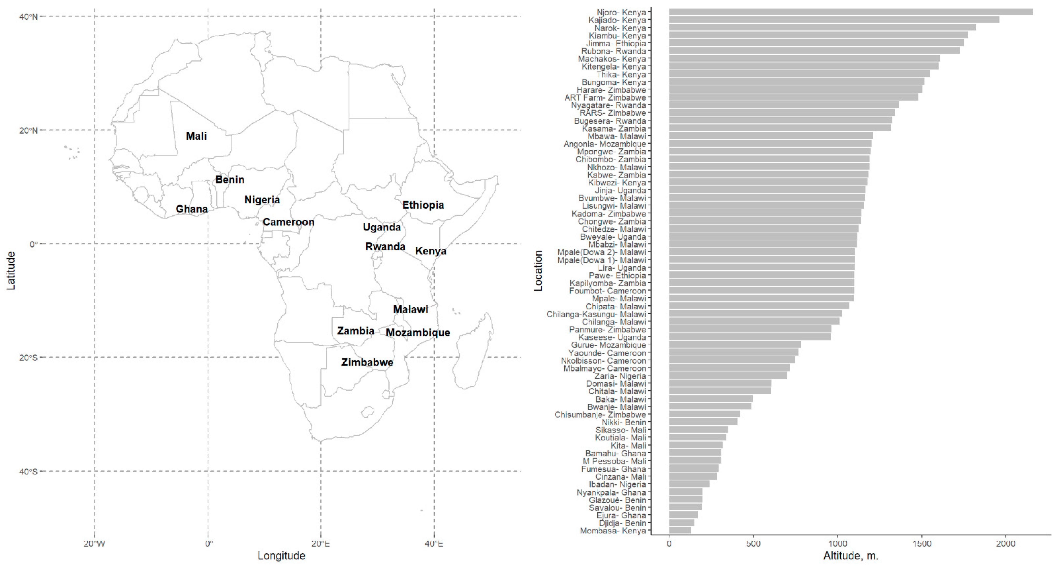
2.1. Pre-Modeling Exploratory Analysis: Soybean Maturity Time

To elucidate the patterns of variation in soybean TTM before the modeling stage, we performed an exploratory analysis of the TTM results for 175 soybean experimental lines using 67 locations of data across 8 cropping seasons (75 environments). Interclass comparisons from an all-fixed-effects model for genotype (G), environment (E), and genotype by environment (G × E), were avoided, as such a model overfitted the TTM response. As an alternative, sequential three-way ANOVA models were used to evaluate the main sources of variability in time to maturity (TTM; days after planting) due to the additive effects of G and E combined.

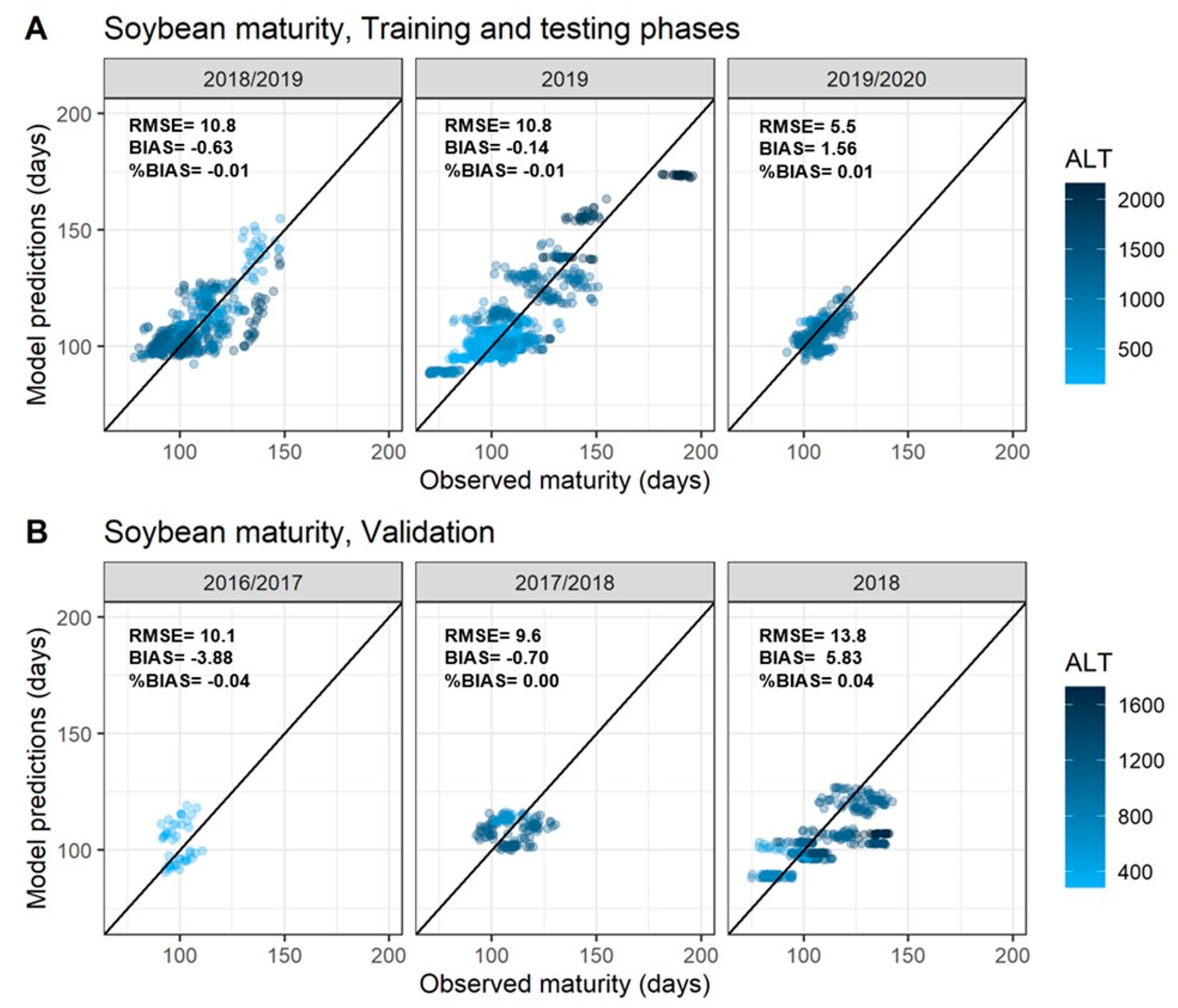
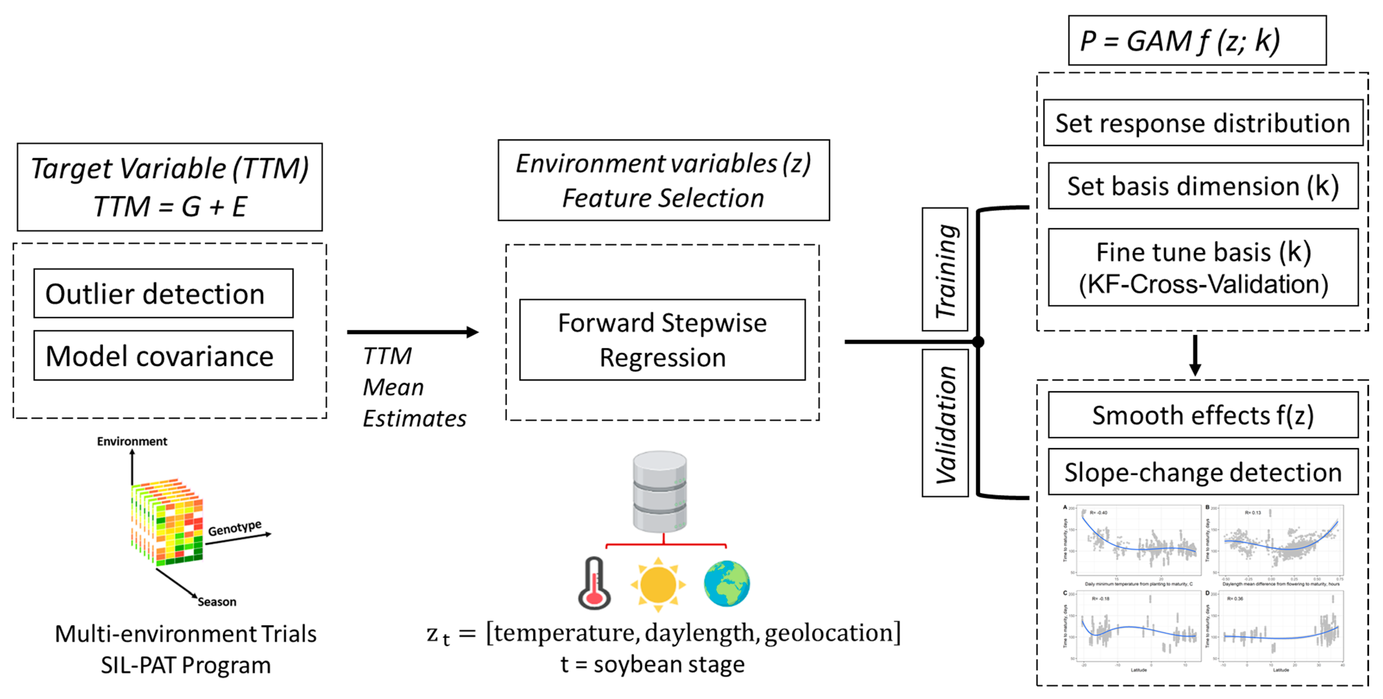
2.2. Modeling Soybean Time to Maturity as a Function of Environment

To prepare the target variable of interest, we obtained TTM mean estimates from a linear model assuming random slope effects for G and E. The random-effects model corrected the departures in TTM for the sample of cultivars and locations evaluated in the MET. This sample is representative of a much larger target population, where the predictive model could be deployed. As such, best linear unbiased predictions (BLUPs) from this process were used to adjust the mean estimates of soybean TTM by accounting for experimental conditions in the MET. Observations which departed unusually from the model assumptions were identified and excluded on the basis of influential observations (Cook’s distance analysis) and residuals vs. fitted maturity time plots. Random-effects models have proven effective for analyzing the phenotypic data generated by a breeding program [16]. Following this step was necessary to make the modeling process more computationally efficient. In this fashion, the first stage of the analysis helped to adequately describe within-environment errors [17], while focusing on enhancing prediction accuracy with a data-driven algorithm in the next steps. Stagewise approaches allow for adjusting cultivar means per trial for later analysis, and enable combined analyses of large amounts of data carrying significant variation across environments [18].

The next step was preparing environmental features for soybean TTM prediction. Weather records were spatially linked to the geographic coordinates (latitude and longitude) of the trialing sites in the SIL–PAT. Soybean cropping conditions were characterized by the geographic and meteorological variables recorded during the growing length cycle. Temperature and daylength are the most physiologically meaningful drivers of phenological changes in soybeans [19], and were included in this analysis. Daily meteorological variables were averaged or summed from planting up to the occurrence of three phenological stages, i.e., emergence, flowering initiation, and physiological maturity. Minimum, maximum, and mean daily temperatures, (°C) were provided by aWhere [20] and validated to ancillary station-based data. Daylength [h day⁻¹] was simulated as a function of latitude based on standard equations by Campbell and Norman [21] and Teh [22]. Aside from absolute values for temperatures and daylength, we considered additional variables capturing the differences in maximum, minimum, and mean daily temperature and daylength, computed between growth stages. For example, DLMEANDIFF signifies the difference in hours of light received from flowering to maturity for a certain cultivar at a given location. A positive value for DLMEANDIFF means that a cultivar was exposed to a longer daylength at flowering than at maturity, because the daylength was becoming shorter during this period. In contrast, a negative value means that a given cultivar received a longer daylength at maturity than at flowering. It must be noted that the SIL–PAT trials were conducted within a considerable latitudinal range (i.e., −21° S–13° N), but still circumscribed to the tropics. Thus, the difference in daylength from flowering to maturity varied between environments from −0.51–+0.71 h.

A full description of all of the variables considered for soybean TTM prediction is presented in

Table 1. Crop cycle seasonal features considered for soybean time to maturity (TTM) predictions.

Temperature (Celsius, °C)
Label	Description	Mean (1 SD)	Range (2 IQR)
TMAXF	Daily maximum temperature to flowering	28.1(2.0)	22.4–32.5 (2.4)
TMINMF	Daily minimum temperature to flowering	19.7 (3.2)	11.2–23.9 (3.8)
TMEANF	Daily mean temperature to flowering	23.9 (2.5)	16.8–28.2 (3.3)
TMAXM	Daily maximum temperature to maturity	28.5 (2.0)	22.5–32.9 (2.8)
TMINMM	Daily minimum temperature to maturity	19.8 (2.8)	11.8–23.9 (3.8)
TMEANM	Daily mean temperature to maturity	24.1 (2.3)	17.2–28.4 (3.4)
Daylength (h, hours)
DLMEANF	Mean daylength to flowering	12.5 (0.5)	11.4–13.3 (0.5)
DLMEANM	Mean daylength to maturity	12.4 (0.3)	11.7–13.1 (0.4)
Difference-based variables (Flowering to Maturity)
TMINMDIFF	Minimum temperature difference (°C)	−0.1 (0.9)	−4, −1.12 (0.5)
TMEANDIFF	Mean temperature difference (°C)	−0.3 (0.7)	−3.5, 1.0 (0.4)
TMAXDIFF	Maximum temperature difference (°C)	−0.4 (0.7)	−3.0, 1.0 (0.6)
DLMEANDIFF	Daylength difference (h)	0.2 (0.2)	−0.5, 0.7 (0.2)
Location-based variables
Long	Longitude, (Degrees, deg)	23.1 (15.6)	−9.5, 38.0 (28.6)
Lat	Latitude, (Degrees, deg)	−5.1 (11.4)	−20.5, 13.1 (21.7)
ALT	Altitude, (Meters, m)	858 (470)	148–2160 (752)

¹ SD: standard deviation; ² IQR: interquartile range (difference between the 75th and 25th percentiles).

.

We ran forward stepwise regression in order to identify the most essential variables that could be combined to build a predictive model of soybean TTM (Supplementary Materials, Figure S4). Redundancy in this set was reduced by removing highly collinear variables via Spearman’s rank correlation. Different feature sets combining a temperature-based predictor at a time, along with DLMEANDIFF and geolocation (latitude and longitude), were evaluated independently. The ”Mallow’s” (C_p), ”Hocking’s” (S_p), and ”Amemiya’s prediction criterion” (APC) indices [23] were used to select the best feature combination. Both C_p and S_p measure the fraction of variability in the response variable (i.e., the residual sum of squares; RSS) that results from recursively fitting models with one regressor removed at a time. The APC index is an adjusted R² that penalizes additional parameters (i.e., degrees of freedom) in the regression’s right-hand side. Lower values for C_p and S_p, and higher values for APC, are equivalent, and indicative of a better model. Variables in the final subset were used as predictors for fitting and parametrizing a generalized additive model (GAM) to predict soybean TTM. Traditional breeding techniques are usually performed on reduced MET datasets due to the few genotypes that are retained for evaluation in the late stages of the trialing process [24]. In our analysis, we avoided losing far too many observations indiscriminately, and favored the application of the GAM statistical algorithm to capture data signals that could be lost with the use of alternative approaches.

The GAM algorithm [25] has been traditionally applied to problems in ecology, land allocation, and climatology [26,27,28]. Given its flexibility and simplicity for capturing complex responses, it is being implemented more often to predict field-level agricultural traits—for example, wheat yield [29], pasture biomass [30], or pest use assessment [31]. Our study is the first documented application of a GAM to predict soybean phenotypic traits across tropical environments. Further, GAMs provide a balanced approach between prediction and explanation. GAMs have been shown to offer a middle ground between highly accurate models with minimal interpretability—such as neural networks—and interpretable models with a tendency to bias (e.g., multiple linear regression). We harnessed the advantages of the GAM methodology in approximating complex non-linear relationships, and evaluated genotype-specific responses to environmental maturity drivers.

Crop breeders model phenotypic expression with a linear modeling framework if phenotypic and environmental data are available. A general version of this approach is:

$$Y=\mu +G+E+\beta E+e$$

(1)

where G and E are mean additive effects relative to the average performance of all of the cultivars across environments, and β represents slope parameters related to cultivar-specific sensitivities to environmental conditions. In this form, Equation (1) is the Finlay–Wilkinson model, or regression on the mean. If specific environmental covariates are available, Equation (1) can be rewritten as a variant of factorial regression:

$$Y=\mu +G+E+\beta z+e$$

(2)

Within this framework, specific sensitivities to each covariate can be modeled independently, and their effects “smoothed” through natural transformations or linear functionals (i.e., a family of functions), such as splines or local regression. A modified version of Equation (2) becomes a GAM of the form:

$$Y=\left[\mu +G+E\right]+f\left(z\right)+e$$

(3)

Following Equation (3), the soybean GAM maturity model was specified as follows:

$$Y_{GE}{}_{\left(ij\right)}\left(z\right)=f\left(z_1\right)+\dots +f\left(z_n\right)={\displaystyle \sum }_i^{N}f\left(z_i;k\right)+ e_{ij}$$

(4)

The response variable Y in Equation (4) is the mean TTM previously adjusted for genotype and environmental effects. Y is predicted with an additive function of the best z-environmental features (e.g., mean temperature to maturity, daylength, etc.). Each predictor (z) is smoothed by a basis function, f, which modulates the maturity response through parameter k. The k parameter is a knot indicating whether there is a change in the direction of the response, and could be tuned, as in other non-parametric approaches, such as splines. The GAM’s advantage is that non-linear relationships carried by the predictors can be easily smoothed to improve model fit, without increasing complexity as in other parametric approaches (e.g., non-linear multivariate regression). GAM-smoothed response curves were generated to facilitate the interpretation of G × E interactions subjacent to the soybean TTM patterns displayed by different cultivars.

Model parametrization was sequential, and used a fivefold cross validation with five replicates to find the optimal knot (k-parameter) for each predictor at a time. For model training and validation, we balanced the number of observations in each dataset, ensuring that trial planting dates be sufficiently represented (Supplementary Materials, Figure S3). Soybean planting in Africa may occur at the end of the year, so that the reproductive stages coincide with the peak of the rainy season in the early months of the subsequent year. However, other regions would grow soybeans during the summer months. In this fashion, the training/testing dataset included observations for the years 2019 (summer season), and 2018/2019 and 2019/2020 (winter seasons). Seasons 2018 (summer), and 2016/2017 and 2017/2018 (winter) were held out for model validation. To account for spatial variability, the latitudinal and longitudinal coordinates of each trial were also included as predictors.

The modeling steps for modeling soybean time to maturity as a function of environment are presented in Figure 1.

3. Results

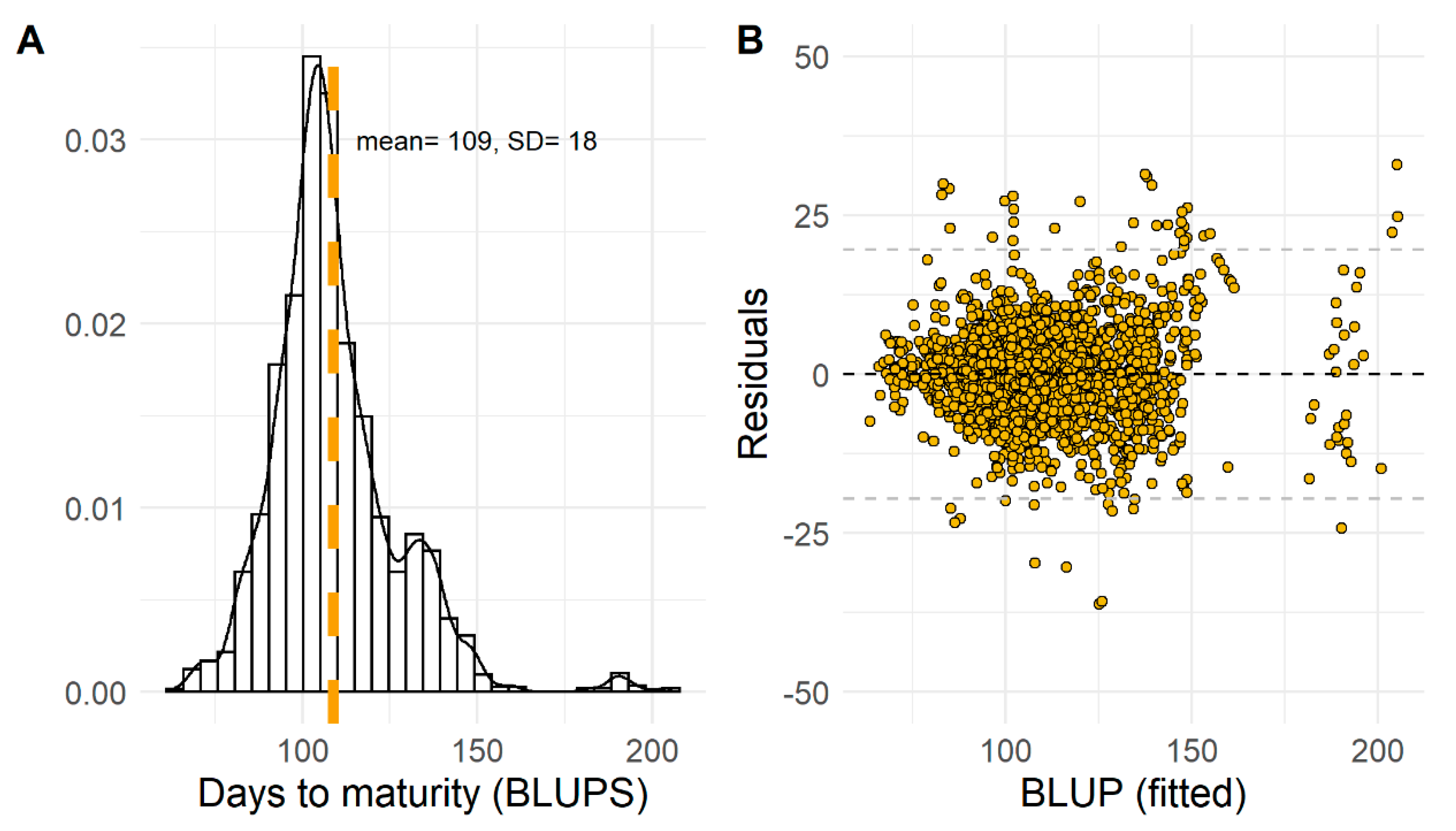
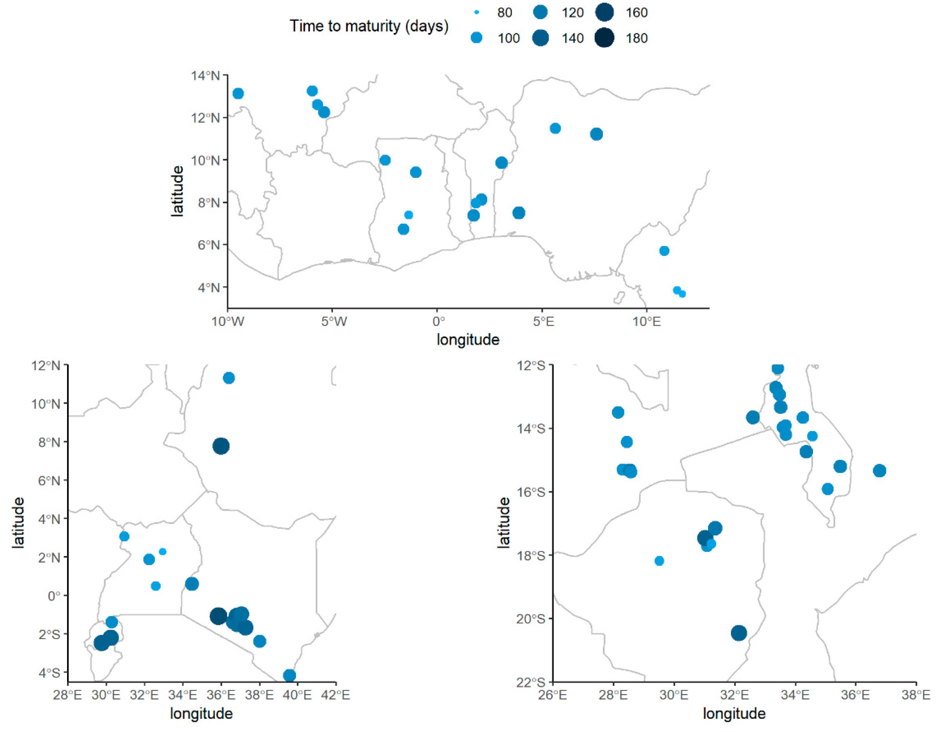
3.1. Exploratory Analysis of Soybean Maturity Timing

A sample size of 250 observations (Genotype × Environment) was used to analyze the sources of variability of the TTM trait recorded in the SIL–PAT dataset (Figure 2 and Figure 3). Genotype (G) and location (L) separately explained 12 and 68% of the total variability in maturity time, respectively. While the contribution of the cropping season (S) alone was low, it helped to account for almost 87% of differences in maturity timing across genotypes and locations (

Table 2. Sources of variation in the target variable soybean time to maturity (TTM). Additive components from G and E are displayed to visualize their relative contribution to TTM variability.

Factor	2 DF Model	2 DF Residuals	1 RSS	Adj-R 2	3 RSE (Days)
Genotype (G)	174	2648	882,623	0.12	18.2
Location (L)	67	2755	330,979	0.68	10.9
Season (S)	8	2814	1,017,289	0.05	19.0
G + L	241	2581	225,891	0.76	9.3
G + S	182	2640	864,933	0.14	18.10
E = L + S	75	2747	280,997	0.73	10.1
G + E	249	2557	121,887	0.87	6.9

² DF = degrees of freedom; ¹ RSS = type II residual sum of squares; ³ RSE = residual standard error.

). Furthermore, the environmental effects (location + season) were almost six times those of genotype, as evidenced by adjusted R^2, and type II sum of squares (SS) estimated in sequential ANOVA models fitted to time to maturity. Expectedly, there was also a gradual decrease in the standard error for the TTM residuals (RSE, Table 2) as additional sources of variability were considered.

Mean TTM was adjusted for hierarchies in the SIL–PAT dataset by means of random-effects modeling. The random-effects model captured these discrepancies efficiently, as 98.5% of the resulting mean TTM met model assumptions (i.e., residuals randomly scattered and bounded within three times the residual SE; Figure 4). Three observations corresponding to the genotype x environment entries L342-Chilanga-2019, N390-Chilanga-2019, and SP 8 DPSB – Thika 2016/2017 failed to meet model assumptions, and were removed from the model. Additional details on outlier detection through residuals and Cook’s distance analysis can be found in the supplementary materials (Figures S1 and S2). The overall soybean mean TTM was 108.9 days after planting [95% CI: 105–113 days] (

Table 3. Soybean time to maturity (TTM) adjusted by genotype (G) and environmental (E) effects. The mean estimates of soybean TTM from this process were used as the target variables in the implementation of the GAM predictive model afterwards.

Random Effects	Group	σ2	σ (days)	σ [95% CI]	n
	G	65.69	8.10	[7.20, 9.16]	175
	E	357.35	18.90	[16.36, 21.92]	73
	Error	47.80	6.91	[6.72, 7.10]
Fixed Effects	Intercept [95% CI]	108.9 [95% CI: 104.87, 113.05]
Goodness of fit	AIC = 19,984
	BIC = 19,918
	R2 = 0.89

, Figure 4). Around the estimated mean, time to maturity departed by 8 and 19 days due to G and E effects, respectively (σ_G, σ_E, Table 3).

The significant pool of variation in maturity occurrence across genotypes and locations in the SIL–PAT (i.e., 89%, Table 3) warranted the exploration of environmental queues that can be used in a parsimonious model to predict maturity times in Sub-Saharan Africa.

3.2. Best Features to Characterize Soybean Time to Maturity (TTM)

The best features to explain changes in TTM were the daily minimum temperature from planting to maturity (TMINM), and the difference in daylength from flowering to maturity (DLMEANDIFF). After also accounting for the effects of latitude and longitude (lat, long), the best subset captured 36% of the differences in maturity reported across genotypes and environments in the SIL–PAT dataset (

Table 4. Best subset of features used as predictors to build a soybean time to maturity (TTM) model. Feature selection based on stepwise forward regression.

Feature Subset	AIC	Adj-R 2	1 Cp	2 HSP	3 APC
TMINM + DLMEANDIFF + lat + long	13,817	0.36	5.04	0.13	0.63
TMEANM + DLMEANDIFF + lat + long	14,014	0.29	7.09	0.14	0.71
TMINDIFF + DLMEANDIFF + lat + long	13,962	0.31	5.0	0.14	0.68
ALT + DLMEANDIFF + lat + long	14,134	0.24	5.0	0.15	0.76

¹ Cp = Mallow’s; ² HSP = Hocking’s; and ³ APC = Amemiya’s prediction indices. Lower numbers denote a better model.

). The actual and fitted soybean TTM responses to each of these four predictors are visualized in Figure 5. Likewise, the best feature subset displayed the lowest numbers for AIC, Cp, HSP, and AP, suggesting that complexity (i.e., the number of parameters) and explanatory capabilities will be balanced in a soybean TTM predictive model built atop this one.

The GAM, using the best explanatory features of soybeans, improved the accuracy of TTM predictions (

Table 5. Evaluation of generalized additive models (GAM) used to predict soybean maturity timing (TTM).

Model	5-Fold Cross Validation				AIC		BIC
	1 RMSE (Days)		R2-Adjusted
	Training	Testing	Training	Testing
lm ~ TMINM	15.34	15.79	0.29	0.30	14,000	14,016
gam ~ f(TMINM, k = 3)	13.55	13.67	0.46	0.46	13,542	13,564
lm ~ (TMINM + DLMEANDIFF)	14.96	15.48	0.32	0.33	13,924	13,945
gam ~ f(TMINM, k = 3) + DLMEANDIFF	12.50	12.70	0.54	0.53	13,280	13,307
gam ~ f(TMINM, k = 3) + f(DLMEANDIFF, k = 3)	10.78	11.02	0.66	0.65	12,793	12,825
lm ~ (TMINM + DLMEANDIFF + lat + long)	14.90	15.48	0.34	0.32	13,817	13,850
gam ~ f(TMINM, k = 3) + f(DLMEANDIFF, k = 3) + lat + long	10.05	10.3	0.70	0.69	12,576	12,620
gam ~ f(TMINM, k = 3) + f(DLMEANDIFF, k = 3) + f(lat, long, k = 4)	9.99	10.35	0.70	0.69	12,564	12,613

¹ RMSE = root-mean-squared error.

). The GAM used three “break points” (i.e., k-nodes) to smooth the overall negative relationship between TTM and both TMINM and DLMEANDIFF. While latitude and longitude show a less than strong association with the response (Figure 5), including two-dimensional smoothing for these terms helped account for the spatial variability due to trial location. Model fit improved as a result.

Following 5-fold model validation, the overall expected TTM for a cultivar tested in the SIL–PAT network was predicted within ±10 days of the observed field data (RMSE = 10.35, Table 5). Relative to simple linear regression, prediction error with the GAM decreased by almost 33%. Likewise, R² increased to nearly 70%, whereas AIC was the lowest among several specifications of the GAM (Table 5). A more detailed description of model agreement during the training and testing phases is presented in Figure 6, and all of the models considered can be found in the Supplementary Materials (Table S1). The GAM predictions fitted acceptably well with the observed time to maturity (Figure 6 and Figure S7). The root-mean-square error (RMSE) ranged between 9 and 14 days at different soybean growing seasons considered in the validation sets (i.e., data held out from training/testing). Relative to other seasons, the model under- and overpredicted time to maturity in 2016/2017 and 2018 by 4% relative to the observed overall mean (x = 109 days, Table 3, Figure 4). The lower fit in 2018 was associated with cultivars tested in mid-to-high-elevation sites in Rwanda (1300–1700 m). In contrast, the less than ideal fit in 2016/2017 was presumably due to fewer cultivars tested at very low elevations in Mali (280–320 m). Overall, soybean TTM predictions held acceptably well for 70% of the 122 genotypes considered for training/testing the GAM (±5 days off the observed maturity). The remaining 30% of the cultivars were off by 6 days or more, and resulted from low sampling, i.e., 15 sites evaluated or fewer.

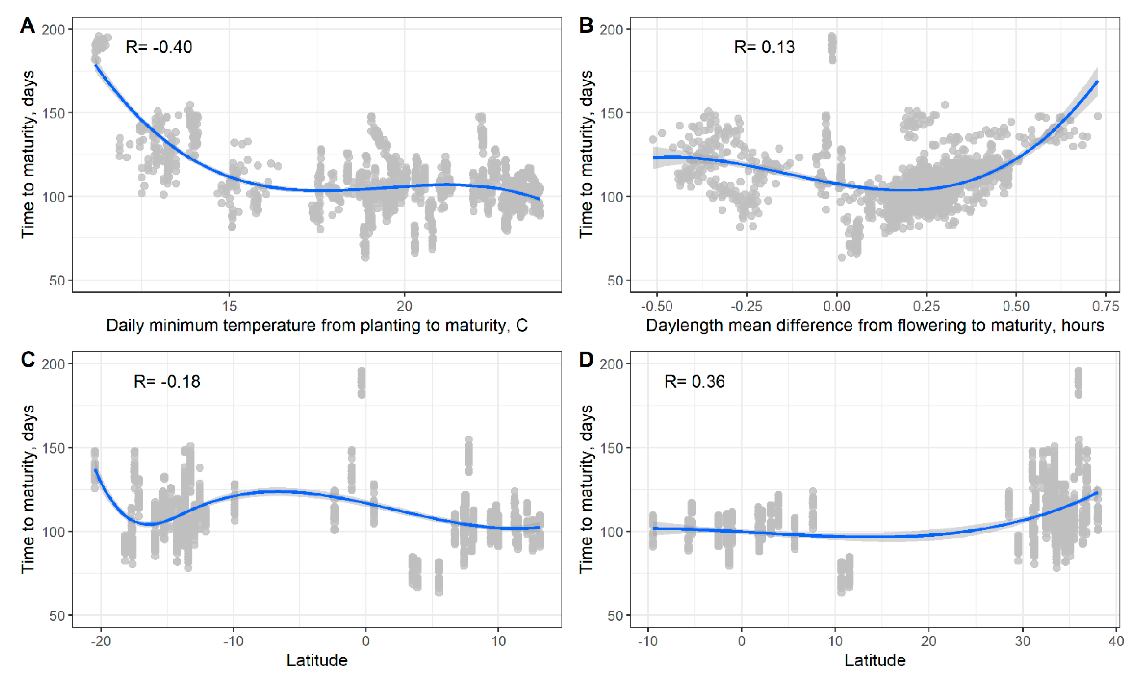
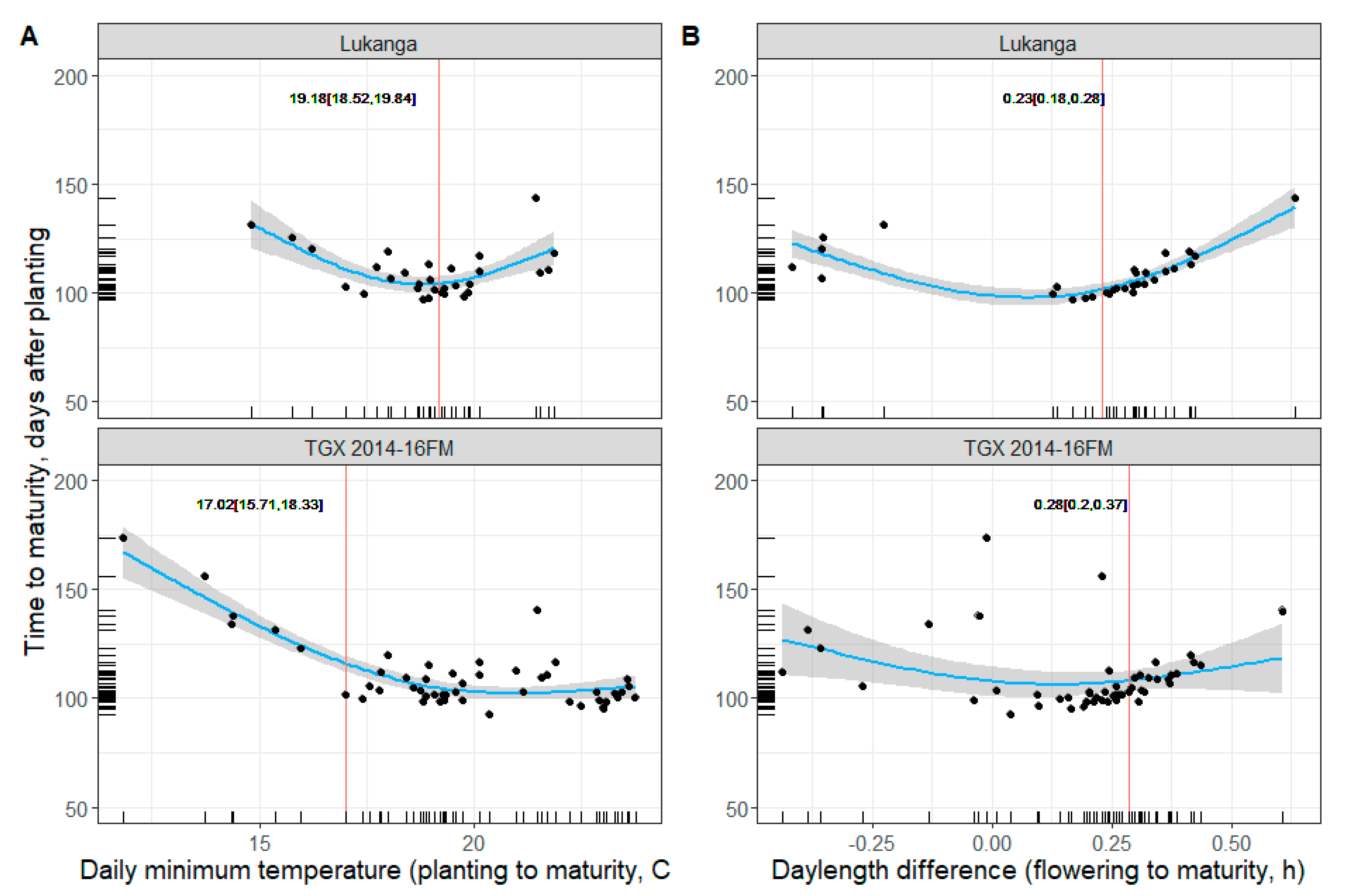
3.3. Soybean Maturity Response to Temperature and Daylength

Cultivars that were tested more consistently across environments (n = 40) captured a larger range of responses, and displayed consistent patterns of maturity occurrence across sites in response to minimum temperature (TMINM) and daylength (DLMEANDIFF). These cultivars were also part of foreign germplasm introduced with the potential for fast introduction to African markets. Segmented regression [32,33] was used to approximate the points in the range of these variables where a shift in response occurred (Appendix A). Critical values where a cultivar responded more sensitively to changes in minimum temperature and daylength were estimated.

To illustrate (Figure 7), the cultivar TGX 2014-16FM reached maturity at around 105 days at sites whose minimum temperatures during the soybean growing cycle were between 17 and 30 °C. In turn, maturity was sharply delayed by almost 60 days in the ~12–17 °C range. The cultivar “Lukanga” displayed a slightly higher value to delimit the ranges of thermal sensitivity (i.e., 19 °C), with seemingly late and early patterns of maturity occurring before and thereafter. In the same vein, physiological maturity occurred more prevalently around 100 days post-planting, when the daylength interval between flowering and maturity (DLMEANDIFF) approached +0.20 h. A positive value for this explanatory variable means that the given cultivars received more light hours at flowering than maturity, and is indicative of their growing cycles progressing along shorter days. As in the case of minimum temperature, cultivars seemed to follow different patterns of TTM response when the gap in daylength between flowering and maturity moved far from a critical value. In the cultivars shown, the critical points of sensitivity to daylength were estimated at +0.23 and +0.28 h of light. Based on an extended analysis, all of the cultivars considered for analysis (Supplementary Materials, Figures S5 and S6) were ranked in terms of their sensitivity to temperature and daylength (i.e., critical points of response). Segmented regression [32,33] was used to approximate the points in the range of these variables where a shift in response occurred.

4. Discussion and Implications

The environment and genotype effects were significant sources of variation in the time to maturity trait. Roughly, the environment (location × season) effects were almost six times more significant than the effects carried by genotype. Our findings are the first to systematically quantify location and genotype effects on soybean maturity time in Africa. Our results corroborate other reports from sub-tropical regions—areas characterized by short days and long summers. Alliprandini et al., (2009), for instance, found that location and genotype accounted for 62% and 29%, respectively, of the variance in the number of days to maturity recorded for commercial cultivars adapted to recurrent cultivation ecoregions in Brazil [34]. While the significance of environmental effects is important in characterizing a phenotype response, inter-cultivar differences are more informative from a breeding perspective [35]. Furthermore, genotype and genotype by environment (G × E) interactions are ubiquitous in phenotypic characterization studies.

G × E effects were revealed by cultivar-specific patterns of maturity that emerged from smoothing the responses attributed to weather features in the GAM. Our results contribute to increasing the understanding of the joint effects of temperature and daylength on the phasic development of soybeans adapted to the African region. Reports from tropical conditions within the same latitudinal circumscription, such as from Hawaii, showed that colder nights (i.e., minimum temperatures in high elevations) extended soybean vegetative periods and delayed physiological maturity (R7) by 25 days [36]. More importantly, we highlighted the seemingly higher importance that thermal variation had relative to photoperiod in characterizing maturity in less hemispheric areas. In fact, low-temperature effects on soybean field development unfold when photoperiodic effects exist but are minimal [37]. A close inspection into critical response values for these areas helped to define ranges of response where the maturity of a cultivar would occur more or less consistently. Such ranges may indicate areas of geographical adaptation for a given cultivar. In turn, sudden shifts in maturity are associated with growing conditions in cultivation areas outside the possible ranges of adaptation.

A cultivar planted under extreme conditions would mature either too early or too late. Consequently, the asynchronous occurrence of maturity leads to incomplete cycles, with detriments on production. Soybean yields, for example, tend to be the highest for cultivars that maximize resources during the whole growth cycle [38]. Low yields can also be the result of premature maturity in short-stature plants that flower too early [39].

Soybean maturity time in the SIL–PAT network can be accurately predicted using geographical and seasonal characterization variables. Statistical learning (i.e., machine learning) can assist in the construction of parsimonious models that replace complex approaches, such as mechanistic models, to readily assist soybean field operations. Alternative approaches, such as mechanistic or process-oriented crop models, can arguably be more accurate under particular conditions, but require a full and detailed description of the physiological processes involved in plant development and growth (i.e., parametrization). Possible accuracy losses from statistical models are compensated for by their lesser demand for inputs and their ease of adaptation to other regions. Accordingly, models need to be constantly updated as the volume of information in their inputs increases. The expansion of the SIL–PAT network, and the information provided within it, will facilitate the validation of the findings from this study. In addition, SIL–PAT protocols encompass data from field-level phenotyping as well as genotypic characterization. In this context, the availability of marker-related data in the coming years could enable the discovery or validation of marker–trait associations in tropical regions for these important traits.

References

1. Carsky, R.J.; Berner, D.K.; Oyewole, B.D.; Dashiell, K.; Schulz, S. Reduction of Striga hermonthica parasitism on maize using soybean rotation. Int. J. Pest Manag. 2000, 46, 115–120. [Google Scholar] [CrossRef]
2. Sinclair, T.R.; Marrou, H.; Soltani, A.; Vadez, V.; Chandolu, K.C. Soybean production potential in Africa. Glob. Food Secur. 2014, 3, 31–40. [Google Scholar] [CrossRef] [Green Version]
3. Khojely, D.M.; Ibrahim, S.E.; Sapey, E.; Han, T. History, current status, and prospects of soybean production and research in sub-Saharan Africa. Crop. J. 2018, 6, 226–235. [Google Scholar] [CrossRef]
4. Foyer, C.H.; Siddique, K.H.; Tai, A.P.; Anders, S.; Fodor, N.; Wong, F.-L.; Ludidi, N.; Chapman, M.A.; Ferguson, B.J.; Considine, M.J.; et al. Modelling predicts that soybean is poised to dominate crop production across Africa. Plant Cell Environ. 2018, 42, 373–385. [Google Scholar] [CrossRef]
5. Keyser, J.C.; Van Gent, R.V. Zambia Competitiveness Report; The World Bank, Environmental, Rural, and Social Development Unit: Washington, DC, USA, 2007. [Google Scholar]
6. Soybean Innovation Lab. Soybean Innovation Lab 2020. Available online: https://www.soybeaninnovationlab.illinois.edu (accessed on 25 February 2021).
7. Tropical Soybean Information Portal. Tropicalsoybean. 2020. Available online: https://www.tropicalsoybean.com/databases (accessed on 25 February 2021).
8. Santos, M.D.F. University of Illinois at Urbana-Champaign Soybean Varieties in Sub-Saharan Africa. Afr. J. Food Agric. Nutr. Dev. 2020, 19, 15136–15139. [Google Scholar] [CrossRef]
9. Leles, E. Pan-African Soybean Variety Trials Database Supports Decision-Making Across Africa. Agrilinks 2021. Available online: https://www.agrilinks.org/post/pan-african-soybean-variety-trials-database-supports-decision-making-across-africa (accessed on 24 February 2021).
10. Ersoz, E.S.; Martin, N.F.; Stapleton, A.E. On to the next chapter for crop breeding: Convergence with data science. Crop. Sci. 2020, 60, 639–655. [Google Scholar] [CrossRef] [Green Version]
11. Zhang, L.X.; Kyei-Boahen, S.; Zhang, J.; Zhang, M.H.; Freeland, T.B.; Watson, C.E.; Liu, X. Modifications of Optimum Adaptation Zones for Soybean Maturity Groups in the USA. Crop. Manag. 2007, 6, 1–11. [Google Scholar] [CrossRef]
12. Mourtzinis, S.; Conley, S. Delineating Soybean Maturity Groups across the United States. Agron. J. 2017, 109, 1397–1403. [Google Scholar] [CrossRef] [Green Version]
13. Cooper, R.L. A delayed flowering barrier to higher soybean yields. Field Crop. Res. 2003, 82, 27–35. [Google Scholar] [CrossRef]
14. Cober, E.R.; Stewart, D.W.; Voldeng, H.D. Photoperiod and Temperature Responses in Early-Maturing, Near-Isogenic Soybean Lines. Crop. Sci. 2001, 41, 721–727. [Google Scholar] [CrossRef]
15. Scott, W.O.; Aldrich, S.R. Modern Soybean Production; S & A Publications: Champaign, IL, USA, 1983. [Google Scholar]
16. Bernardo, R. Reinventing quantitative genetics for plant breeding: Something old, something new, something borrowed, something BLUE. Heredity 2020, 125, 375–385. [Google Scholar] [CrossRef] [PubMed] [Green Version]
17. Piepho, H.-P.; Möhring, J.; Schulz-Streeck, T.; Ogutu, J.O. A stage-wise approach for the analysis of multi-environment trials. Biom. J. 2012, 54, 844–860. [Google Scholar] [CrossRef]
18. Buntaran, H.; Piepho, H.; Schmidt, P.; Rydén, J.; Halling, M.; Forkman, J. Cross-validation of stagewise mixed-model analysis of Swedish variety trials with winter wheat and spring barley. Crop. Sci. 2020, 60, 2221–2240. [Google Scholar] [CrossRef]
19. Major, D.J.; Johnson, D.R.; Tanner, J.W.; Anderson, I.C. Effects of Daylength and Temperature on Soybean Development 1. Crop. Sci. 1975, 15, 174–179. [Google Scholar] [CrossRef]
20. aWhere | Climate Smart Weather Insights Backed by AI. 2021. Available online: https://www.awhere.com/ (accessed on 25 February 2021).
21. Campbell, G.S.; Norman, J.M. An Introduction to Environmental Biophysics; Springer: New York, NY, USA, 2000. [Google Scholar]
22. Teh, C.B.S. Introduction to Mathematical Modeling of Crop Growth: How the Equations Are Derived and Assembled into a Computer Model; Brown Walker Press: Boca Raton, FL, USA, 2006. [Google Scholar]
23. Amemiya, T. Selection of Regressors. Int. Econ. Rev. 1980, 21, 331. [Google Scholar] [CrossRef]
24. Dawson, J.C.; Endelman, J.B.; Heslot, N.; Crossa, J.; Poland, J.; Dreisigacker, S.; Manès, Y.; Sorrells, M.E.; Jannink, J.-L. The use of unbalanced historical data for genomic selection in an international wheat breeding program. Field Crop. Res. 2013, 154, 12–22. [Google Scholar] [CrossRef] [Green Version]
25. James, G.; Witten, D.; Hastie, T.; Tibshirani, R. (Eds.) Moving Beyond Linearity. In An Introduction to Statistical Learning: With Applications in R; Springer: New York, NY, USA, 2013; pp. 265–301. [Google Scholar]
26. Roberts, M.J.; Key, N. Agricultural Payments and Land Concentration: A Semiparametric Spatial Regression Analysis. Am. J. Agric. Econ. 2008, 90, 627–643. [Google Scholar] [CrossRef]
27. Stauffer, R.; Mayr, G.J.; Messner, J.W.; Umlauf, N.; Zeileis, A. Spatio-temporal precipitation climatology over complex terrain using a censored additive regression model. Int. J. Clim. 2017, 37, 3264–3275. [Google Scholar] [CrossRef] [Green Version]
28. Lawler, J.J.; White, D.; Neilsonjand, R.P.; Blaustein, A.R. Predicting climate-induced range shifts: Model differences and model reliability. Glob. Chang. Biol. 2006, 12, 1568–1584. [Google Scholar] [CrossRef] [Green Version]
29. Chen, K.; O’Leary, R.A.; Evans, F.H. A simple and parsimonious generalised additive model for predicting wheat yield in a decision support tool. Agric. Syst. 2019, 173, 140–150. [Google Scholar] [CrossRef]
30. De Rosa, D.; Basso, B.; Fasiolo, M.; Friedl, J.; Fulkerson, B.; Grace, P.R.; Rowlings, D.W. Predicting pasture biomass using a statistical model and machine learning algorithm implemented with remotely sensed imagery. Comput. Electron. Agric. 2021, 180, 105880. [Google Scholar] [CrossRef]
31. Rosenheim, J.A.; Cass, B.N.; Kahl, H.; Steinmann, K.P. Variation in pesticide use across crops in California agriculture: Economic and ecological drivers. Sci. Total. Environ. 2020, 733, 138683. [Google Scholar] [CrossRef]
32. Muggeo, V.M.R. Segmented: An R Package to Fit Regression Models with Broken-Line Relationships. R News 2008, 8, 20–25. [Google Scholar]
33. Küchenhoff, H.; Carroll, R.J. Segmented Regression with Errors in Predictors: Semi-Parametric and Parametric Methods. Stat. Med. 1997, 16, 169–188. [Google Scholar] [CrossRef]
34. Alliprandini, L.F.; Abatti, C.; Bertagnolli, P.F.; Cavassim, J.E.; Gabe, H.L.; Kurek, A.; Matsumoto, M.N.; De Oliveira, M.A.R.; Pitol, C.; Prado, L.C.; et al. Understanding Soybean Maturity Groups in Brazil: Environment, Cultivar Classification, and Stability. Crop. Sci. 2009, 49, 801–808. [Google Scholar] [CrossRef]
35. Malosetti, M.; Ribaut, J.-M.; Van Eeuwijk, F.A. The statistical analysis of multi-environment data: Modeling genotype-by-environment interaction and its genetic basis. Front. Physiol. 2013, 4, 44. [Google Scholar] [CrossRef] [PubMed] [Green Version]
36. George, T.; Bartholomew, D.; Singleton, P. Effect of temperature and maturity group on phenology of field grown nodulating and nonnodulating soybean isolines. Biotronics 1990, 19, 49–59. [Google Scholar]
37. Lawn, R.; Byth, D. Response of soya beans to planting date in south-eastern Queensland. II.* Vegetative and reproductive development. Aust. J. Agric. Res. 1974, 25, 723–737. [Google Scholar] [CrossRef]
38. Egli, D. Cultivar maturity and potential yield of soybean. Field Crop. Res. 1993, 32, 147–158. [Google Scholar] [CrossRef]
39. Sinclair, T.R.; Hinson, K. Soybean Flowering in Response to the Long-Juvenile Trait. Crop. Sci. 1992, 32, 1242–1248. [Google Scholar] [CrossRef]
40. Muggeo, V.M.R. Estimating regression models with unknown break-points. Stat. Med. 2003, 22, 3055–3071. [Google Scholar] [CrossRef] [PubMed]
Figure 1. Steps to implement a generalized additive model (GAM) to predict soybean time to maturity (TTM), based on seasonal characterization and resources from a breeding program in Africa.
Agronomy 11 01043 g001
Figure 2. Countries, trial sites, and altitudes, considered for a soybean maturity prediction model adapted to soybeans grown in African conditions (Soybean Innovation Lab, Pan-African Variety Trials: SIL–PAT, 2015–2020).
Agronomy 11 01043 g002
Figure 3. Geographical variation of soybean time to maturity (TTM) in the Soybean Innovation Lab Pan-African Variety Trials (SIL–PAT) network.
Agronomy 11 01043 g003
Figure 4. Soybean time to maturity (TTM) mean estimates, including best linear unbiased predictions (BLUPs) from an all-genotype–environment random-effects model (Panel A). Residuals of the random-effects model (Panel B). Dashed horizontal lines are the upper and lower threshold limits bounded within 3 SE. Mean TTM estimates were used as the target variable in the GAM soybean TTM model.
Agronomy 11 01043 g004
Figure 5. Soybean time to maturity (TTM) responses to crop cycle seasonal features used as the best predictors in a GAM. For visualization, panels (AD) show the non-linear effects for each variable smoothed via natural splines (k = 3).
Agronomy 11 01043 g005
Figure 6. Implementation of a generalized additive model (GAM) to predict soybean time to maturity in African growing environments. Panel (A) shows results from the training/testing phases. Panel (B) shows results for model validation (i.e., environments held out from the training/testing) process. The color bar on the right-hand side indicates the range of elevations for the sites considered in the model (altitude; ALT (m)).
Agronomy 11 01043 g006
Figure 7. GAM-smoothed response of soybean time to maturity (TTM) to seasonal variables during the growing cycle. Each dot represents a testing site where the given cultivar was evaluated. Red parallel lines indicate a change in the direction of the response, and were approximated through segmented regression (Appendix A).
Agronomy 11 01043 g007