Expansion and Specialization of Agricultural Systems in Western Mediterranean Areas: A Global Analysis Based on the Two Last Census Data

Abstract

The study aims to describe and interpret the agricultural system dynamics on the Western Mediterranean areas in terms of occupied land and crop specialization, by using the available data from the two last agricultural censuses. From the spatial point of view, we chose to adopt the most detailed level available, by using the smallest land administrative unit (LAU) for every involved country (Spain, Portugal, France and Italy). The resulting database was made of about 16k records and seven fields for a total of 112k single data. The considered variables were: total farm area (TFA), utilized agricultural area (UAA), irrigated area (IA), arable lands (AL), permanent crops (PC), permanent grassland (PG) and remaining surface (RS). The LAU data analysis was carried out following the four steps: (i) level of land occupation by agricultural systems; (ii) patterns of crop groups in UAA composition; (iii) attribution to each LAU of an agricultural typology (AT), resulting from the combination of the two previous features and iv) calculation of two synthetic indices to evaluate the expansion and specialization level for each LAU. Finally, an analysis of the spatial distribution of the two indices was proposed. Results showed a lowering over time of the TFA, UAA and PG areas and an increase of IA and RS. The number of identified ATs was rising at the expense of their extension. This phenomenon led to a fragmentation in ATs spatial distribution within the same geographical region. These changes prove that farmers’ responses to the driving forces acting on agricultural systems have been more differentiated than in the past. The prevailing strategy seems to aim at a reduction in the level of specialization of the agricultural systems whereas less marked was the lowering of their level of expansion.

1. Introduction

Mediterranean agriculture shows peculiar traits due to climate, soil nature, orography, traditional food production, etc., which are rooted in history and allow to distinguish it from the agricultural systems in other European regions [1]. These particular features together with farming practices (e.g., irrigation, varieties choice and seed timing), makes suitable the cultivation of a large range of crops [2]. Among them, there are temperate crops (wheat, barley, potatoes, vegetables, etc.), subtropical crops (maize, rice, tobacco, etc.) and permanent crops (citrus fruits, olive, grape, etc.), which are often complemented with an extensive presence of fodder crops aimed at to sustaining livestock (especially sheep and goats).

Consequently, the alternatives for farmers are numerous and it is not easy to define a single model for Mediterranean agriculture since many different agricultural systems are pursued simultaneously, and often they coexist in a same region producing a complex landscape mosaic [3]. Farms are often highly specialized in typical productions with worldwide significance for their nutritional, commercial and cultural value and therefore different cropping systems can coexist in the same location, even at the local scale [1]. This wide range of suitable crops is confirmed by the high level of plant biodiversity that characterizes Mediterranean habitats with an outstanding flora diversity of 15–25 thousand species, almost half of which are considered threatened, endangered or vulnerable [4].

In the last decades, Mediterranean agricultural systems have experienced significant changes in terms of land use and crop composition, under the pressure of driving forces acting on a global scale such as worldwide market competition, climate change and the need to contain environmental impact [5]. On the other hand, other phenomena operate on a local scale. For instance, besides soil erosion, all the major land degradation processes are present within the Mediterranean basin such as soil sealing, salinization, desertification and rapid urban sprawl [6,7]. In addition, nature of the soil and slope steepness can just affect the choice of the crop to be grown [8].

Finally, the interaction between biophysical variables and socioeconomic conditions further enhances the complexity of the Mediterranean environment [9] resulting in a diversified pattern of land systems, which are difficult to synthetize and evaluate because of their extreme variability in space and time.

To explain this variability and to identify emerging trends, the analysis of land-cover and land-use changes (LCLUCs) has been applied successfully in several countries [10] and especially in the Mediterranean ones because of its particular climatic and morphogenetic conditions and historical anthropogenic pressure [9,11]. Two opposite trends have been generally observed on agricultural system dynamics, even at farm level [12]: (i) farmland abandonment and (ii) intensification of farming practices [13,14]. The former is typical of the marginal, internal, hilly areas, where the profitability of agriculture has become uncertain, whereas the latter occurs in the fertile, irrigated coastal plains where the conditions allow for higher profitability and the proximity of urban areas and touristic centers ensures a high and stable demand for food.

Deepening the knowledge of agricultural land use dynamics and the incidence evolution of the different crop groups is precious in evaluating the effects on ecosystem service provision, CAP efficacy and soil conservation policy [15,16,17].

For this purpose, different data sources can be used such as farm accountancy data networks (FADN) and land parcel identification systems (LPIS) [18,19,20]. However, none of these databases is exhaustive from a spatial or a statistical point of view. FADN considers just a small sample of the existing farms and LPIS considers only the farms accessing to CAP payments. Attempts to use the national agricultural census have been fewer because of the difficulty to harmonize data from methods differing each other for the surveyed items or the crop-group composition. The use of the census data at the most detailed level for which information was available (municipalities) implies to process a considerable amount of records that has discouraged the application on a large scale of this type of analysis, which is generally approached only at the national level.

Another limit in using census data is the lack of information about intensification of agricultural activity. According to [21], land-use intensity is a multidimensional factor that encompasses different aspects interlinked with each other that, if considered separately, lead to a misleading appraisal of this phenomenon. In particular, (i) inputs to the production system (land, labor and capital), (ii) outputs from the production system (yields), and (iii) changes in ecosystem properties (non-marketed ecosystem services) should be considered in measuring the intensity level of agricultural systems [21,22,23] (Erb et al., 2013; Kuemmerle et al., 2013; Rega et al., 2020). Unfortunately, many of these data are not available on the same scale on which land-cover data are available and this is the reason because land system changes have been mainly focused on land-cover changes [22,24] (Kuemmerle et al., 2013; Levers et al., 2018). The only information about agricultural system intensity that can be gained from census data is that related to the expansion of farmland or cultivated/irrigated area that represent only one strand of land-use intensity.

The aim of this study is to describe and interpret the agricultural system dynamics within the Western Mediterranean region in terms of expansion and crop composition, by using the two last agricultural censuses available for the involved countries (France, Italy, Portugal and Spain). This survey was carried out at the most detailed level, by using the smallest land administrative unit (LAU) available in order to obtain an accurate picture of the situation and to identify the trajectories drawn by agricultural systems during a 10-year span period.

2. Materials and Methods

2.1. Study Domain

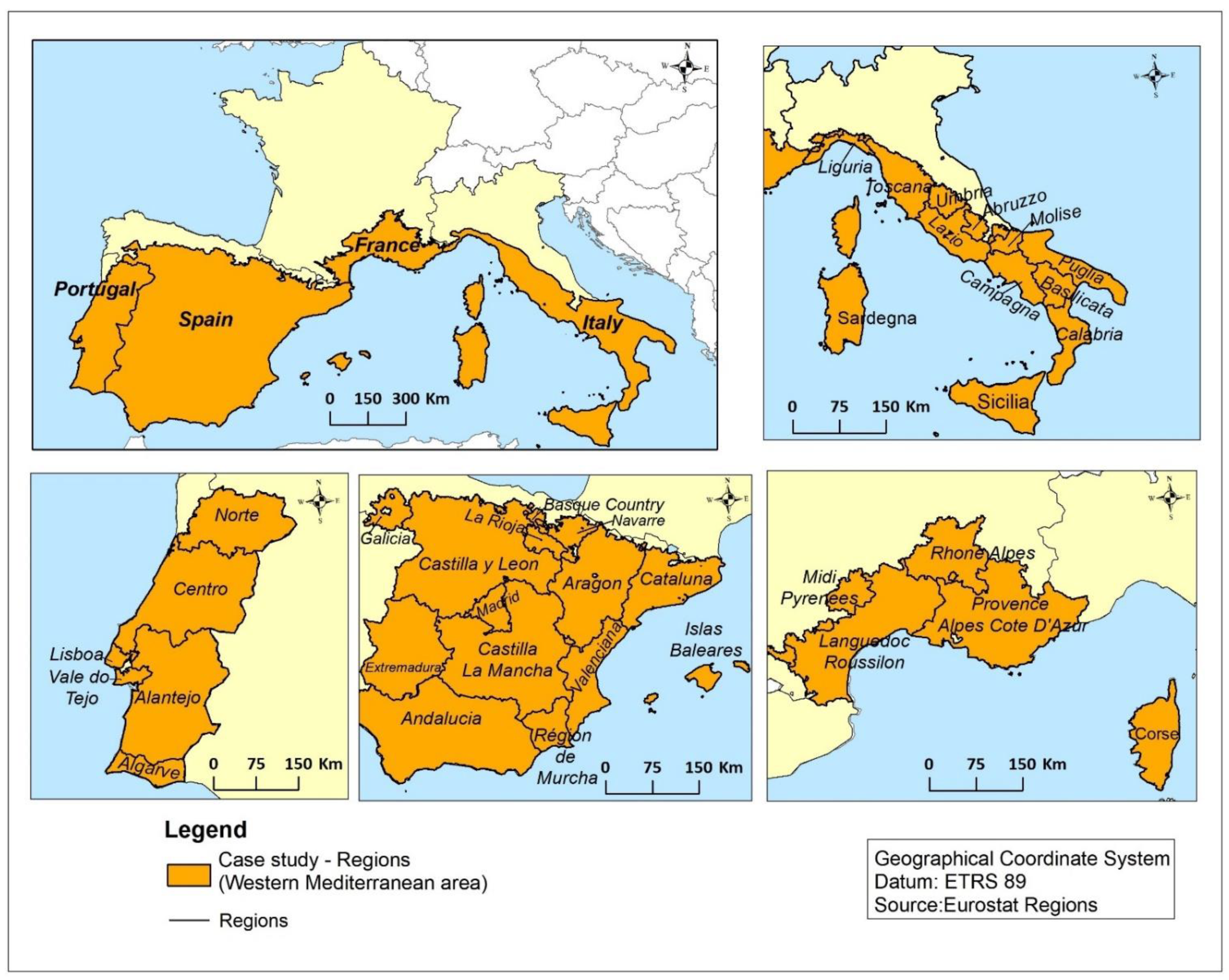
We limited the study to four Western European Mediterranean countries: Portugal, Spain, France and Italy. Although these countries have significant differences within them, they also show similarities from the historical and socioeconomic point of view [25]. In this way, we intended to reduce the influence of cultural or political factors due to the country refer to and enhance the effects produced by the biophysical conditions in order to verify the existence of possible transnational behaviors.

The borders of the Mediterranean area were selected according to the Natura 2000 Biogeographical Mediterranean Region [26], which is essentially based on ecological criteria. The domain of study, obtained through an overlay between the above-mentioned delimitation and the national map of administrative units (Figure 1), included almost the entire territory of Portugal (95% of the national surface) and Spain (90%), about a half of the territorial surface of Italy (56%) and a smaller portion of France (11%) (

Table 1. National surface, surveyed surface (in kha and %), land administrative units (LAUs) (in number and %), and the average size of LAU for each country.

Countries (-)	National Surface (kha)	Surveyed Surface (kha)	Surveyed Surface (%)	LAU (Number)	LAU (%)	Average Size of LAU (ha)
Portugal	9221.2	8799.8	95.4	2484	15.0	3543
Spain	50,599	45,601.5	90.1	7354	44.4	6201
France	64,380.1	7278.2	11.3	3342	20.2	2177
Italy	30,133.8	16,929.2	56.2	3400	20.5	4979
Total	154,334.1	78,608.7	50.9	16,580	-	5061

). The considered area amounts in total to 154.3 million ha with more than half belonging to Spain (58% of total), about a fifth to Italy (22%) and the remaining portion equally divided between Portugal (11%) and France (9%).

About the time span, the analysis had been restricted to the two last agriculture censuses available for the considered countries. The censuses had not been carried out everywhere in the same years. In Spain and Portugal, the years of the two last censuses were 1999 and 2009, whereas in France and Italy the censuses were carried out in 2000 and 2010. Consequently, data were pooled according to the census release to which they referred to, penultimate and last census (C1 and C2, respectively), rather than to the year in which data were really collected.

Regarding the choice of the LAU level, we decided to consider the most detailed level available for each national census. In particular, the following LAUs were used for the different countries: municipio (ES), commune (FR), comune (IT) and freguesia (PT). According to European [23,27], this level (LAU = 2) corresponds to the municipality for most countries except for PT where the freguesia is a submunicipality unit. In this way, we wanted to save, as far as possible, the actual heterogeneity of the Mediterranean agricultural systems by limiting the effect of compensations due to the choice of a too large land unit size.

2.2. Data Collection

Census data at the highest level of administrative unit were not stored by the statistical office of the European Union (Eurostat) [27], so we started to acquire a database already implemented by another research group [27] who have worked on larger study-area containing seven Mediterranean countries (Spain, Portugal, France Italy, Malta, Algeria and Tunisia). In this way, some problems concerning changes in administrative units over time (deletion, fusion, resizing, renaming, etc.), unmatched codifications of LAUs between census datasets and georeferenced maps or the alignment of different national geographical projection were overcome.

In order to improve the consistency/comparability of data and to deepen the knowledge of the spatial distribution of agricultural systems in the Western European area, we operated some modifications to the original database.

The official websites of each country were explored to verify correctness and meaning of the items used in the census survey and the real correspondence among the categories adopted (https://www.ine.pt/; https://www.ine.es/; http://agreste.agriculture.gouv.fr/recensement-agricole-2010/resultats-donnees-chiffrees/; http://dati.istat.it/ accessed on 10 August 2019). The composition of each crop group (arable lands, permanent crops and permanent grassland) used for each national census were checked and reconstructed, when needed, to avoid inappropriate comparisons. Moreover, to improve the data consistency, missing data were requested to the respective statistic offices or calculated (for instance in the case of arable land for French LAUs).

Finally, the need to gather data from different countries forced us to create a new code for identification of each record, since the national codifications of the administrative units differed greatly from country to country.

The new database (PostgreSQL) consisted of 16,580 records, one for each LAU falling within the study area, and 7 fields, one for each considered variable coming from the census data.

The differences among national administrative systems affected the LAUs’ size and therefore the ground resolution of each unit sampling was different for each country. In particular, the average size of LAU ranged from a minimum of 2177 (for a French LAU) to 6201 ha (for a Spanish LAU). Although these differences were not negligible, the range of variation can be considered acceptable and the comparison among the LAUs coming from different countries appeared legitimate. An indirect confirmation of the validity of this assumption comes from the distribution of LAUs’ number among the countries of origin (Table 1). Almost half of them belonged to Spain (44%), about 20% to Italy and France and the remaining 15% to Portugal. These percentages were close to those calculated in terms of surveyed surface, with differences (percentage by surface minus percentage by number) rather contained (SP = +14%, IT = +1%, PT = −4% and FR = −11%).

The list of the variables that constituted the new database is reported in

Table 2. The considered variables (name, code and description), the normalization method used to generate the corresponding indicators and the index to which they refer.

Variable	Code	Description	Normalization	Indicator	Index
Territorial Extension	TE	Total surface of the LAU	-	-	-
Total Farm Area	TFA	Total surface belonging to farmers	TFA/TE	TFA’	EXP
Utilized Agricultural Area	UAA	Total cultivated surface	UAA/TFA	UAA’	EXP
Irrigated Area	IA	Irrigated portion of the UAA	IA/UAA	IA’	EXP
Arable Lands	AL	Total seeded (or transplanted) surface	AL/UAA	AL’	SPE
Permanent Crops	PC	Woody crops lasting for several years	PC/UAA	PC’	SPE
Permanent Grassland	PG	No seeded fodder crops	PG/UAA	PG’	SPE
Remaining Surface	RS	Portion of UAA devoted to other uses a	RS/UAA	RS’	SPE

^a calculated as RS = (UAA − (AL+PC+PG)).

.

We considered three variables related to the land use: (i) total farm area (TFA); (ii) utilized agricultural area (UAA); (iii) irrigated area (IA) and four variables related to land cover: (iv) arable lands (AL); (v) permanent crops (PC); (vi) permanent grassland (PG) and vii) remaining surface (RS), calculated as remaining portion of UAA (RS = UAA − (AL + PWC + PFC)). The meaning of all variables is in accordance with the definitions given by the Eurostat Agriculture Glossary (https://ec.europa.eu/eurostat/statistics-explained/index.php?title=Category:Agriculture_glossary accessed on 27 August 2019). The only exception is RS that is not mentioned in Eurostat Agriculture Glossary but it can be assimilated to “kitchen garden” (KG), defined as the complement to UAA (UAA = AL + PC + PG + KG). Therefore, RS that is a residual category inside which different land-cover types may fall such as, for instance, temporary non cultivated areas. For this reason, we preferred to give a wider significance to RS rather than consider it only as a surface cultivated by smallholders or householders for self-consumption purpose.

All variables concerning the livestock size were excluded from this analysis because those data were not directly referable to land surfaces. We added to the database also the field of the territorial extension (TE) of each LAU obtained by matching each record of the database with the European georeferenced dataset of administrative units (https://ec.europa.eu/eurostat accessed on 20 April 2021).This variable, although not involved in the analysis, was used to normalize the TFA (see below).

To differentiate data from the two censuses, we added “1” as index to the name of variables resulting from the C1 (e.g., UAA₁ = utilized agricultural area in 1999 or 2000) and “2” to the name of those from the C2 (e.g., UAA₂ = utilized agricultural area in 2009 or 2010).

2.3. Data Processing

In order to verify adequacy of the database resulting from the merge of data from each national census, numerous checks were made by considering the fulfilment of a series of irrefutable conditions. Analyses of data consistency are included in the Supplementary Materials (Table S1). Some discrepancies were observed for the LAUs where TFA was bigger than TE (TE ‒ TFA < 0). These inconsistencies (6.4 and 4.5% on the total number of LAU, for C1 and C2 respectively) can be explained with the fact that the agricultural census ascribes all the farm surface to the spatial unit where the farm headquarter is, even if some fields can be located in neighboring municipalities.

The LAUs where UAA = 0 have been excluded from the analysis as they can be considered non-agricultural (376 LAUs for C1 and 399 LAUs for C2).

The main descriptive statistics (mean, median, mode, max, min, standard deviation, variability coefficient, skewness and kurtosis) were calculated for the 7 considered variables, and they are reported on in the Supplementary Materials (Table S2).

To eliminate the effect of LAUs’ different territorial extension, all variables were normalized according to the roles showed in Table 2. Each normalized variable was transformed in an indicator (Table 2), whose value was obtained by assigning a growing rank (1, 2, 3 and 4) according to the interval in which the value of the normalized variable fell. For this purpose, we divided the entire range of variability of normalized variable (0-1) into four intervals of equal size: [0.00–0.25), [0.25–0.50), [0.50–0.75) and [0.75–1.00]. If the value of the normalized variable was higher than 1.00 (this case occurred for the TFA of some LAUs as reported above) we assumed that the class to assign was equal to 4. The choice of using equal intervals to classify the normalized variables instead of, for examples the quartiles, gave us the advantage of creating indicators that were independent on the data distribution in the particular case study. Indeed, the indicators thus calculated can be compared with those obtained from other studies and they maintain an objective meaning clearly interpretable.

From the first three variables (TFA, UAA and IA) we obtained as many indicators of intensity in agricultural land-use (LUI), whereas the indicators of agricultural system composition (LCC) were generated from the variables related to land-cover (AL, PC, PG and RS). The notation of the indicators, tough keeping the name of variable from which it derives, is distinguishable from use of the single quote mark (‘), as shown in Table 2.

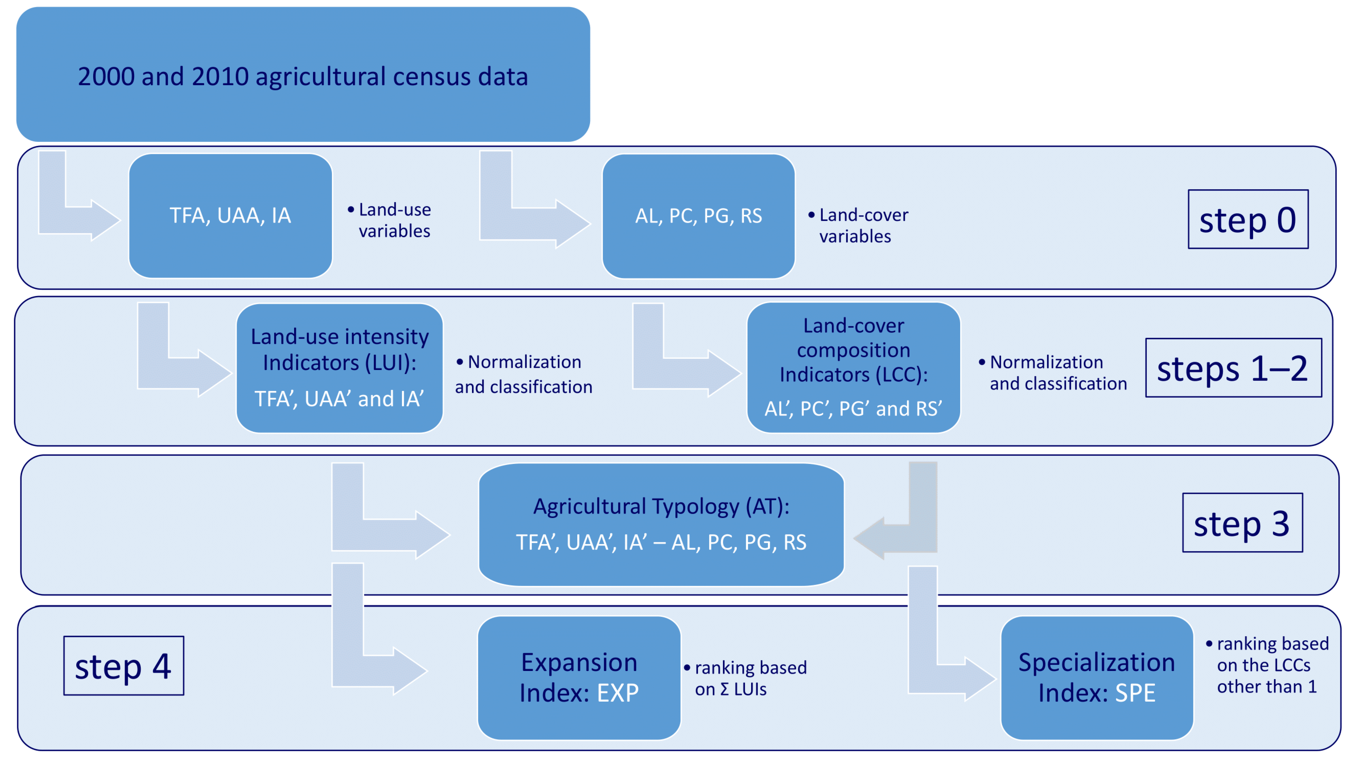
The analysis of agricultural systems resulting from the indicator creation had been carried out by following a conceptual path developed in four steps: (i) evaluation of land use intensity; (ii) evaluation of crop patterns; (iii) identification of agriculture typologies and (iv) analysis of expansion and specialization of agricultural systems by calculating specific indices (Figure 2).

The first one concerned the intensity level in land and water use attributable to each LAU. The three indicators were selected in order to identify: (i) how much of the territorial extension of each LAU was devoted to an agricultural use (TFA’); (ii) what portion of the total farm area was really cultivated (UAA’) and (iii) what portion of the cultivated area was really irrigated (IA’).

The second step was aimed to evaluate the incidence of the four main crop groups (AL’ = arable land; PC’ = permanent crops; PG’ = permanent grassland and RS’ = remaining surface) on the UAA composition, in order to describe the crop profile of each LAU and to define its main productive sectors.

The third one was devoted to assign a typology (AT) to agricultural systems identified in each LAU. AT was constituted by a string of 7 numbers ranging from 1 to 4 obtained by merging the values of all the indicators TFA’ UAA’ IA’ - AL’ PC’ PG’ RS’, the hyphens is used to separate the LUI from LCC indicators. The LUIs can assume all ranking values (1, 2, 3 or 4) and therefore 64 (= 4³) different combinations were possible, whereas LCCs can generate only 34 combinations because they were all normalized by using the same variables (UAA) and their sum cannot be higher than 7 otherwise they would exceed 100% of the UAA (Σ LCCs ≤ 7). At the end, the number of the possible ATs was equal to 2176 (64 × 34).

Finally, in order to provide a synthetic evaluation of the level of intensity in land/water use and the degree of specialization ascribable to agricultural systems for each LAUs, the four steps had been dealing with. At this purpose, two indices were calculated: the index of expansion (EXP) and the index of specialization (SPE). The first one was calculated as the sum of the three LUIs (EXP = Σ LUIs) and it was recodified to assume 5 different values (

Table 3. The method used to calculate EXP and SPE indices starting from the indicator (LUI and LCC) values.

Σ LUIs	EXP Value	Combinations of LCC Values	SPE Value
3 or 4	1	one 2 and three 1 a	1
5 or 6	2	two 2 and two 1 b	2
7 or 8	3	three 2 and one 1 c	3
9 or 10	4	one 3 and three 1 d	4
11 or 12	5	one 3 one 2 and two 1e	5
		one 4 and three 1f	6

Possible combinations: ^a 2111, 1211, 1121, 1112; ^b 2211, 2121, 2112, 1221, 1212, 1122; ^c 1222, 2122, 2212, 2221; ^d 3111, 1311, 1131, 1113; ^e 3211, 3121, 3112, 2311, 1321, 1312, 2131, 1231, 1132, 2113, 1213, 1123; ^f 4111, 1411, 1141, 1114.

). The second one was obtained by considering the values of LCCs other than 1 regardless of their position in the AT string, and it was recodified to assume 6 different values (Table 3). Based on the two indices, we operated a reclassification of the LAUs into 30 groups (resulted from the product of 5 values of EXP by 6 values of SPE) that represented synthetically the total variability of the Mediterranean agricultural system database.

Finally, the alphanumeric database was spatialized through a GIS (ArcGIS v. 10.2 by ESRI), in order to evaluate the geographical distribution of the data and understanding their spatial correlation. Consequently, each record of the original database was matched with the georeferenced dataset of administrative units used for the extraction of TE. In this way, it has been possible to obtain a unique coverage of the whole study area. In this way, we created the maps with the distribution of the two indices (EXP and SPE) for the two census dates.

3. Results

3.1. Land Use and Land Cover Variables

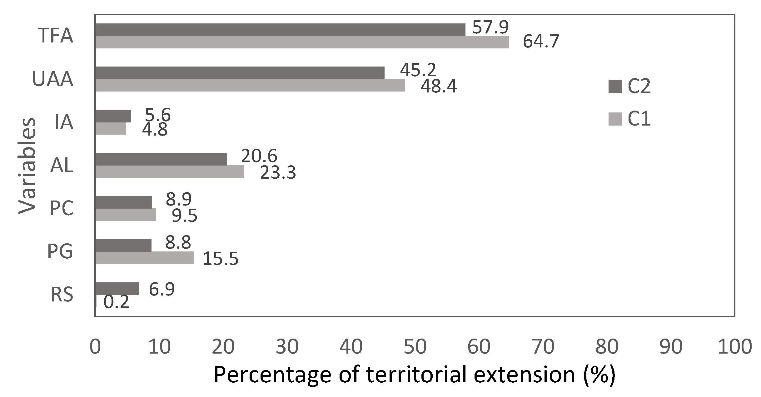
Figure 3 shows the percentage of territorial extension attributable to each variable for the two census dates. The data of C1 and C2 were directly comparable because the exclusion of LAUs with UAA = 0 left substantially unchanged the value of TE (78.50 M of ha for TE₁ and 78.48 M of ha for TE₂).

During the considered 10-year span period, we can observe a clear decline for almost all the variables considered. The TFA₂ lost about 5.39 M of ha and −11% as a difference in percentage rate between the two dates ((TFA₂ ‒ TFA₁) / TFA₁ × 100)) passing from 64.7% of the TE to 57.9. The UAA₂ showed a similar dynamic, although more limited both in relative and absolute terms (−2.51 M of ha and −7% in comparison with the UAA₁). On the other hand, we observed an increase of IA₂ (+0.62 M of ha and +16% in comparison with IA₁). This result became even more significant (+25%) if we related IA to the extension of UAA instead of TE, which had on the same period an opposite trend (IA₂ = 12.4% of the UAA₂ whereas IA₁ = 10.0% of UAA₁).

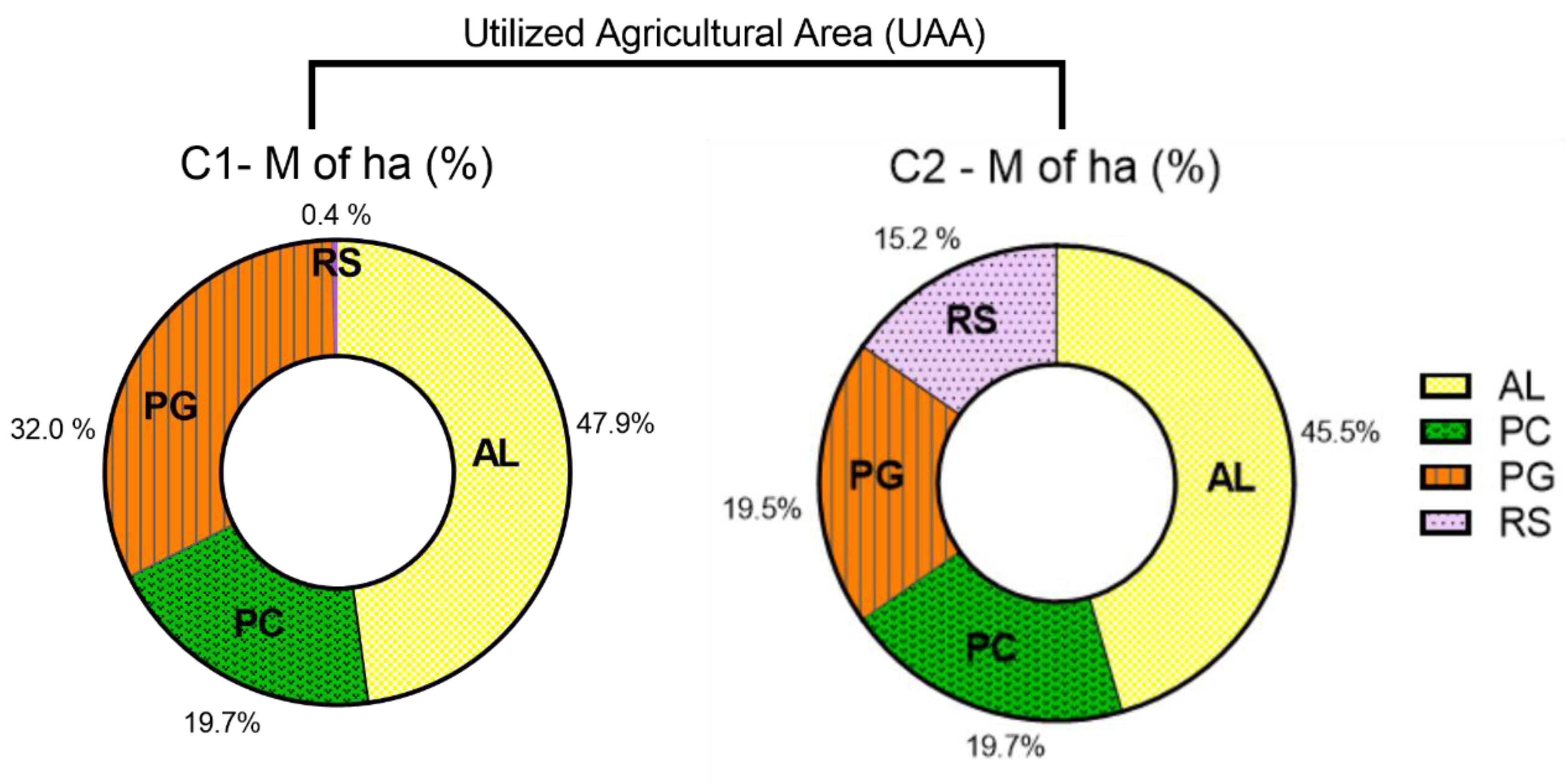
In terms of land cover variables (Figure 4), the PG was the crop group with the highest decrease (−5.27 M of ha lost by PG₂ in comparison with PG₁), followed by the AL (−2.03 M of ha) and the PC (−0.49 M of ha), whereas the surface occupied by the RS gained 5.27 M of ha in the passage from C1 to C2. These differences led to a significant change in UAA composition (Figure 4). The PG₁, which represented 32.0% of UAA₁, nearly halved their incidence (PG₂ was 19.5% of UAA₂), whereas the RA₂ increased its relative extension more than 40 times, passing from the 0.4% of the UAA₁ to 15.2% of the UAA₂. The contribute of the other two crop-groups remained substantially constant over time and AL and PC constituted respectively about little less than half and a fifth of the UAA, for both the census times.

3.2. Step 1 and 2: Evaluation of LUI and LCC Indicators

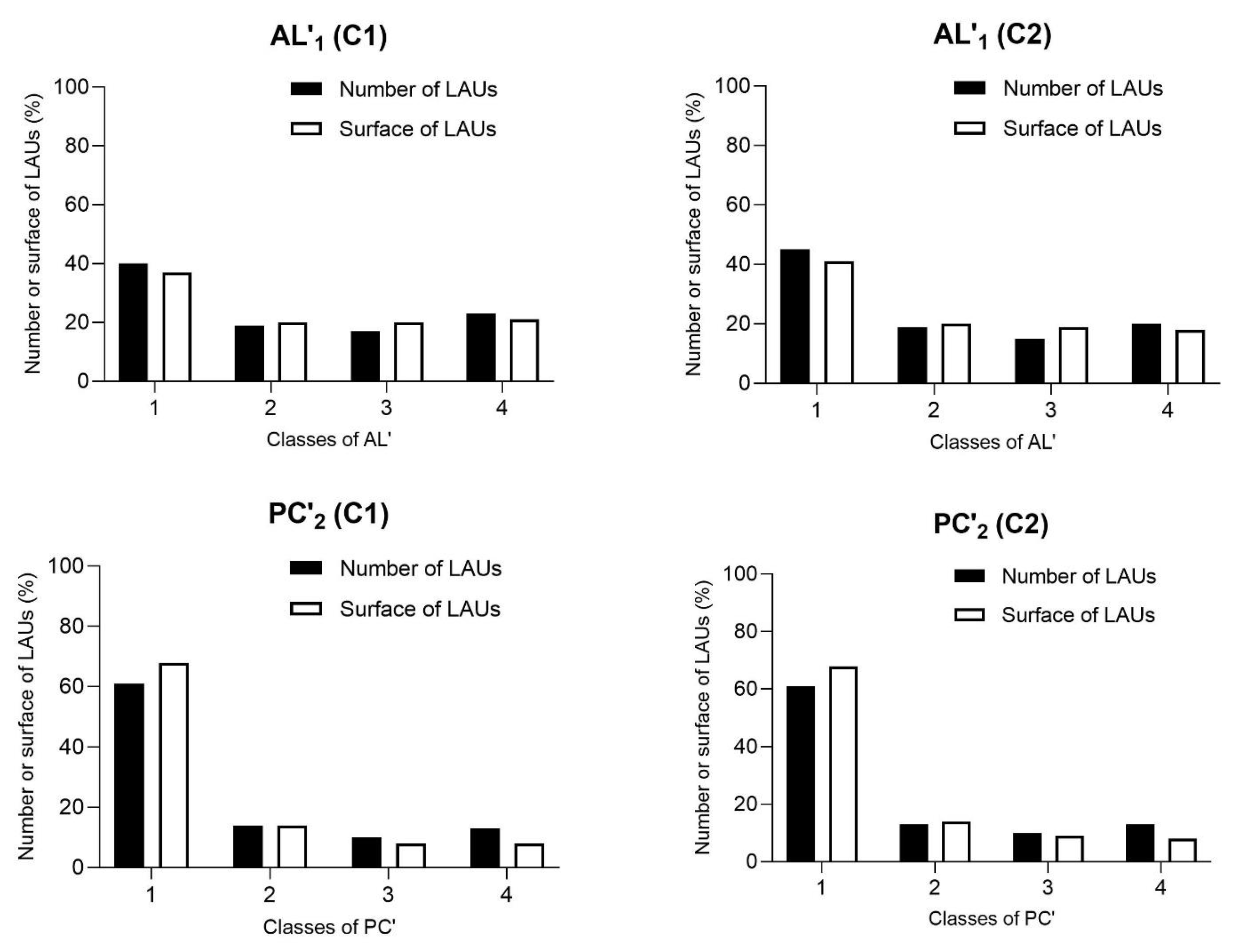
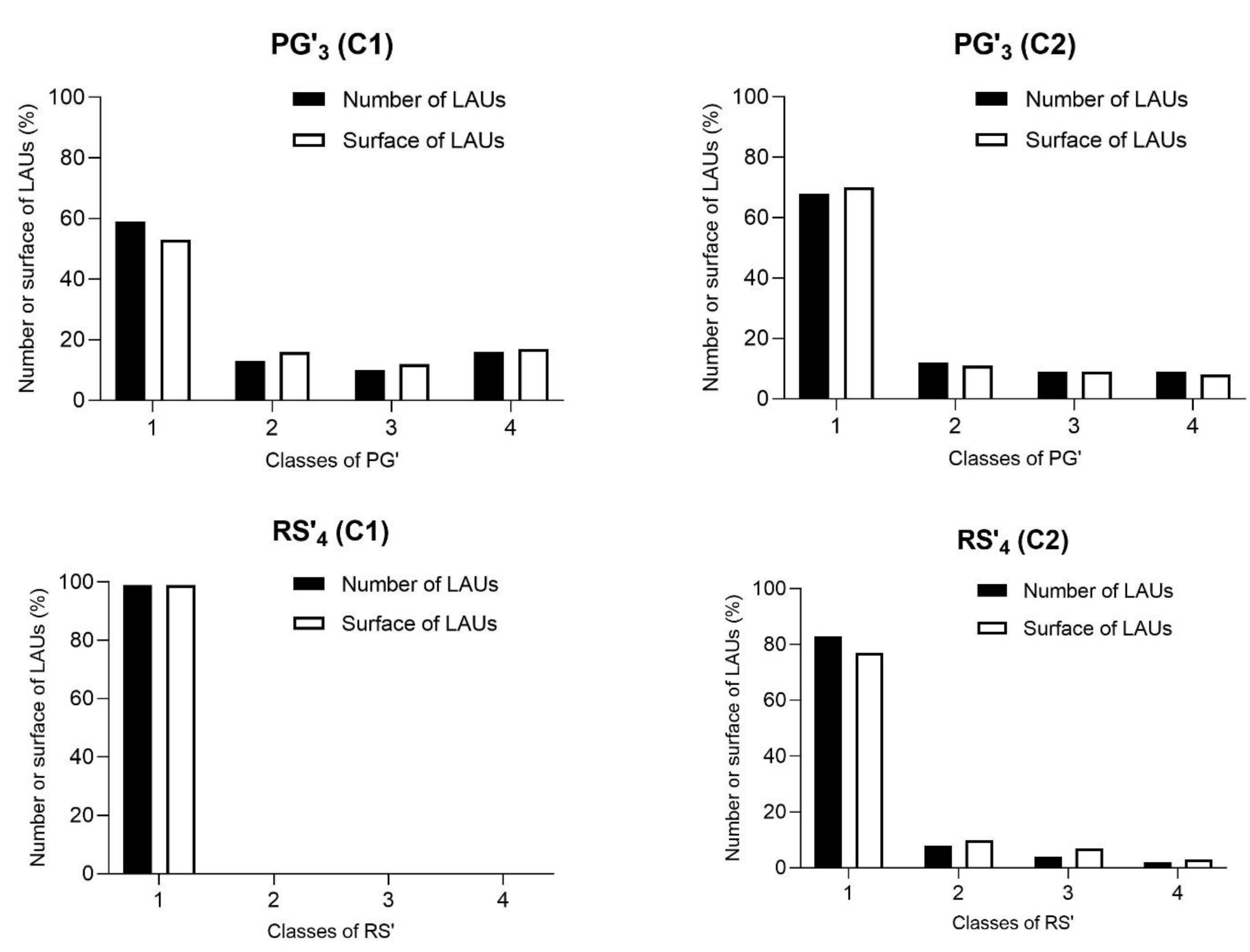
Figure 5 and Figure 6 show the percentage distribution of LAUs in terms of number and surface into the four size classes for each indicator.

The pattern of LAU number was substantially similar between the two census periods (C1 and C2) but rather different between the two indicator typologies (LUI and LCC). The LCCs (Figure 5) had a high decrease of LAU number passing from the 1st class (0–25% of UAA) to the 2nd class (25–50% of the UAA). The differences among the other classes were negligible and sometimes a slight increase can be observed for the 4th class (75–100% of the UAA). Generally, these trends were more evident for the RS’ (99.7% in the 1st class for C1) and less pronounced for the AL’ (41%, 19%, 17% and 23% of total LAU’s number still in C1).

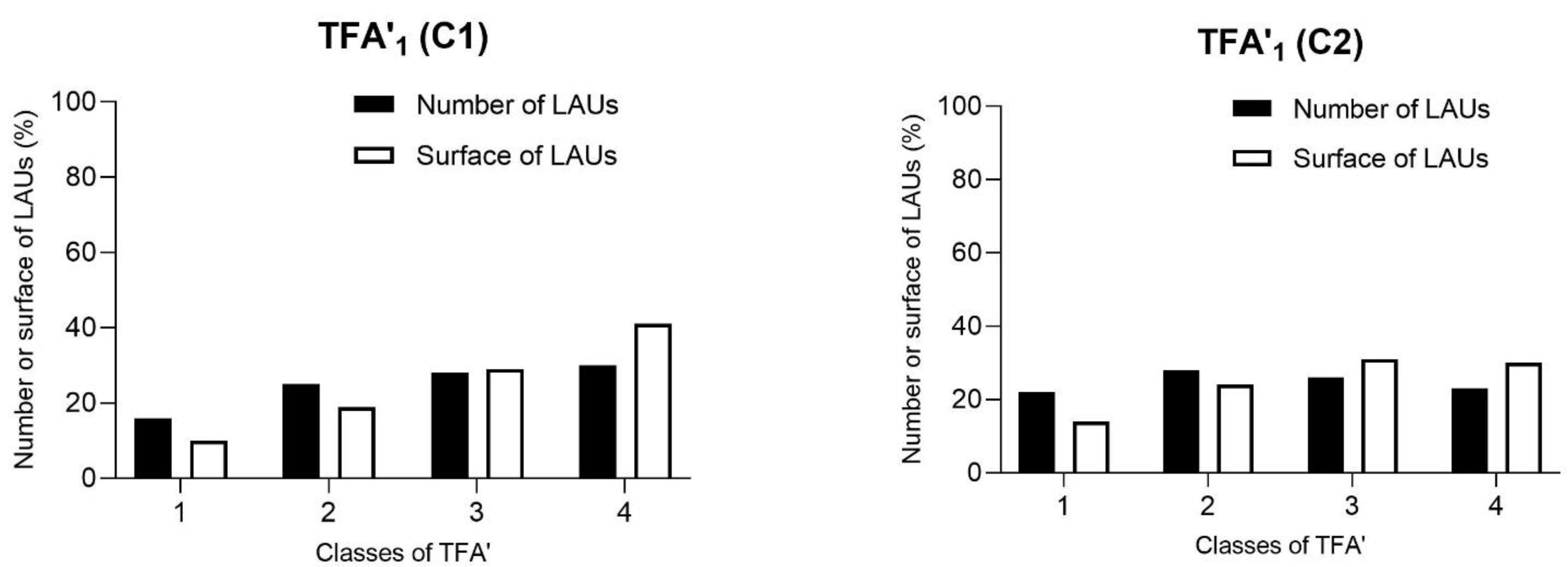
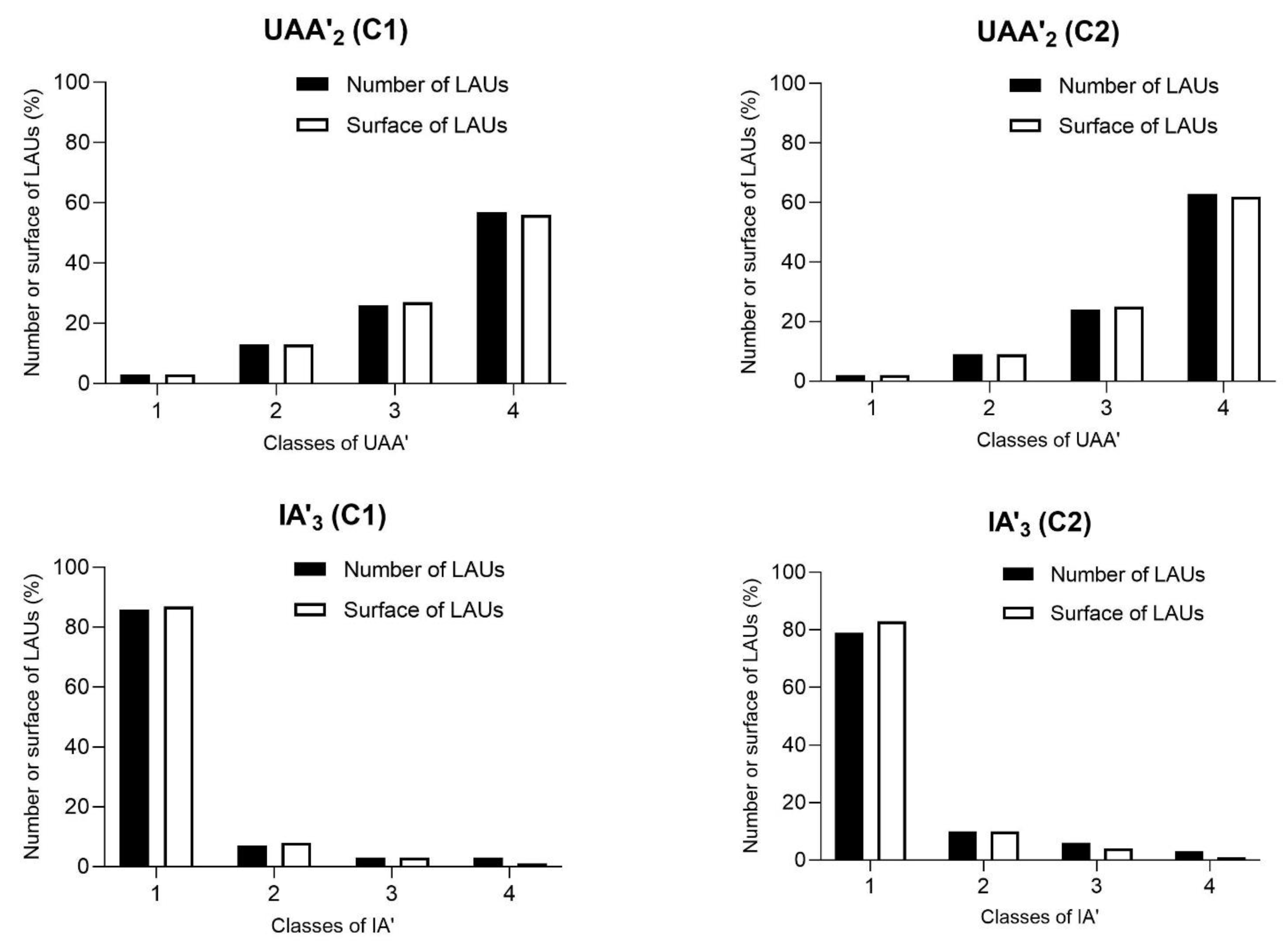
Conversely, the LUIs (Figure 6) showed a radically different behavior. The distribution of LAU number was quite stable among the four size classes for the total farm area (TFA’) (16%, 25%, 29% and 30% and 22%, 28%, 26% and 23%, for C1 and C2, respectively). Most of the LAUs (58% and 64% for C1 and C2, respectively) showed a percentage of utilized agricultural larger than 75% of TFA, whereas very few LAUs had an irrigated area (IA’) higher than 50% or 75% of UAA (from 3% to 6% of LAU number, by considering both dates).

If we consider the territorial extension of the LAUs involved instead of their number, it is evident that the trends do not change by confirming the efficacy of normalization process in making indicator results independent of the LAU’s size.

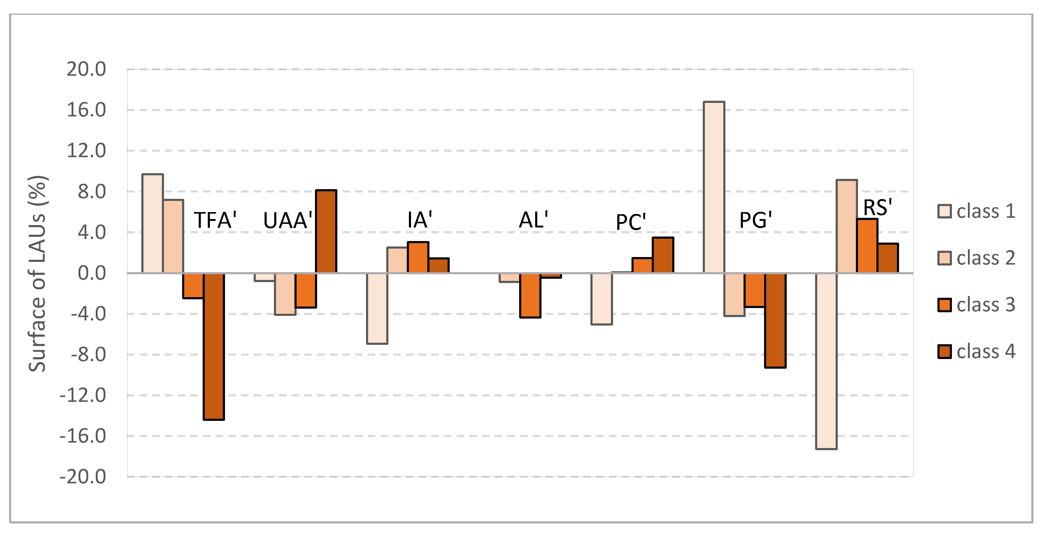
Regarding the changes in the pattern distribution of indicators over time (Figure 7 and Figure 8), the variations were coherent with the trends observed for the variables of origin (decrease of TFA and PG, increase for IA and RS), even if these differences were generally contained. The readjustment of LAUs’ number or surface resulted in an increase of the 1st class in face of the highest classes of intensity (3rd and 4th) for TFA’ and PG’, whereas an opposite trend was drawn by IA’ and RS’. Passing from C1 to C2, the most relevant differences at level of LAU’s number (Figure 7) were recorded for TFA’ (+6.2% and −6.6% for the 1st class and 4th, respectively), IA’ (−6.9% for the 1st class), PG (+8.6% for the 1st class) and RS’ (−15.8% and +8.7% for the 1st and 2nd, respectively). About the surface distribution (Figure 8), the percentage changes were higher for the 2nd and 4th class of TFA’ (+4.9% and −10.5%, respectively), for the class 4th of UAA’ (+6.3%), for the 1st and 4th class of PG’ (+17.4% and −9.7%, respectively) and for the 1st, 2nd and 3rd class of RS’ (−22.1, +10.6 and +7.7%, respectively)

3.3. Step 3: Individuation of Agricultural System Typologies

The seven indicators were combined obtaining 657 and 913 different combinations for C1 and C2, respectively. This means that among the 2176 possible ATs, only about one third (30% for C1 and 40% for C2) has been really identified within the study area.

Table 4. The most representative agricultural typology (AT) identified for the first census date (C1) in terms of number of LAUs (>%1 of the total number) and surface of LAUs (> 1 M of ha).

ATs in C1	Number of LAUs (n)	Number Percentage (%)	ATs in C1	Surface of LAUs (M of ha)	Surface Percentage (%)
441-4111	1218	7.4	441-4111	5.9	7.5
341-4111	612	3.7	441-1141	3.0	3.8
441-1141	455	2.8	341-4111	2.8	3.5
141-1141	387	2.3	441-3121	1.9	2.4
241-1141	324	2.0	431-1141	1.7	2.2
241-4111	313	1.9	441-2131	1.6	2.1
341-1411	292	1.8	421-1141	1.4	1.8
341-1141	289	1.8	141-1141	1.4	1.8
241-1411	264	1.6	241-4111	1.4	1.7
441-3121	240	1.5	341-1141	1.3	1.6
441-1411	222	1.3	341-3121	1.2	1.6
441-2131	213	1.3	331-1141	1.2	1.6
			441-3111	1.2	1.5
			431-4111	1.2	1.5

and

Table 5. The most representative agricultural typology (AT) identified for the second census date (C2) in terms of number of LAUs (>%1 of the total number) and surface of LAUs (>1 M of ha).

ATs in C2	Number of LAUs (n)	Number Percentage (%)	ATs in C2	Surface of LAUs (M of ha)	Surface Percentage (%)
441-4111	964	5.9	441-4111	5.2	6.7
341-4111	673	4.1	341-4111	3.4	4.3
141-1141	373	2.3	241-4111	1.6	2.1
241-4111	328	2.0	141-1141	1.3	1.6
241-1141	287	1.7	241-1141	1.3	1.6
241-1411	275	1.7	341-3111	1.1	1.4
141-1411	254	1.5	241-1411	1.1	1.3
341-1411	244	1.5	341-1411	1.0	1.3
			141-1411	1.0	1.3

show the most diffuse ATs both for number (>%1 of the total number) and surface of LAUs (>1 M of ha) for the two census dates (C1 and C2).

The AT 441-4111 was the most representative both in number of LAUs and surface involved for the two census dates. It was characterized by a high agricultural land-use (TFA’ and UAA’ = 4th class), a scarce use of irrigation (AI’ = 1st class) and a clear prevalence of arable land (4th class) over other crop-groups (all in 1st class). We can identify this AT as a rainfed agricultural system devoted to annual herbaceous crop cultivation. The AT 341-4111, which differed from the previous one only for a lower value of TFA’ (3rd class), was the second combination for importance occupying the third position in C1 and the second one in C2 (both for LAUs’ number and surface extension). This means that the agricultural system maintained the same crop composition of the previous one, but with a lower incidence of agricultural lands, comparing to other land uses such us urban ones. Additionally, the AT with an even lower TFA’ (241-4111) was quite widespread (9th in C1 and 3rd in C2 for both parameters) confirming that the high level of agricultural lands and the limited use of irrigation coupled with herbaceous crop rotations remained the most relevant system according to the Mediterranean agro-pedoclimatic conditions.

ATs such as 141-1114 and 241-1114, in which the RS’ prevailed within a context characterized by a low incidence of agricultural land use (TFA’ = 1st or 2nd class), but with a high index of cultivation (UAA’ = 4th class), were largely represented in C2 (3rd and 4th position in both rankings) and, to a lesser extent, in C1 (8th and 9th position). Instead, the ATs oriented towards permanent grassland (441-1141, 431-1141, 421-1141 and 341-1141) occupied high positions C1, but lost much of their importance over time (none of these was at the top of the C2 ranking). In addition, the mixed agricultural systems (with at least two LCCs not belonging to the 1st class), which reached a significant diffusion in C1 (Table 4, were 441-3121, 441-2131 and 341-3121, but they disappeared from the C2 ranking (Table 5).

Finally, agricultural systems with a high presence of permanent crops (PC’ = 2nd, 3rd or 4th class) did not occupy a good rank in any chart.

Generally, it seems to be evident that a contraction (both in the LAUs’ number and in the occupied surface) of the most widespread ATs occurred in C2 because of both the TFA decrease and the growing number of ATs identified.

3.4. Step 4: Calculation of EXP and SPE Indices

The results of the indices calculation for each LAU are reported in

Table 6. Number and surface of LAUs falling in each class of the two indices (EXP and SPE) and relative percentage calculated on the total values for the first census date (C1).

Class of EXP	LAU Number (n)	LAU Number (%)	LAU Surface (M of ha)	LAU Surface (%)	Class of SPE	LAU Number (n)	LAU Number (%)	LAU Surface (M of ha)	LAU Surface (%)
1	667	4.0	2.26	3.0	1	20	0.1	0.07	0.1
2	4379	26.6	16.75	21.3	2	1235	7.5	6.27	8.0
3	7059	42.8	34.78	44.3	3	219	1.3	1.06	1.4
4	4048	24.6	23.37	29.8	4	1728	10.5	9.32	11.9
5	321	1.9	1.24	1.6	5	4596	27.9	24.13	30.7
					6	8676	52.7	48.00	37.7

. Most of the LAUs showed an average degree of land-use intensity, as they belonged to the class 3 of the EXP (42.8% and 45.0% in C1 and C2, respectively), followed by the classes 2 and 4 with very similar values (26.6 and 24.6% in C1; 26.4% and 22.7% in C2), whereas the classes 1 and 5 showed much lower frequencies (4.0 and 1.9% in C1; 3.9% and 2.0% in C2). The SPE showed completely different behavior. Generally, we observed a larger number of LAU on the more specialized classes, with little differences between the two census times. In C1 (Table 6), the first three class represented less than 10% of the total number of LAUs whereas class 6 represented more than half of all LAUs (52.7%).

In C2 (

Table 7. Number and surface of LAUs falling in each class of the two indices (EXP and SPE) and relative percentage calculated on the total values for the second census date (C2).

Class of EXP	LAU Number (n)	LAU Number (%)	LAU Surface (M of ha)	LAU Surface (%)	Class of SPE	LAU Number (n)	LAU Number (%)	LAU Surface (M of ha)	LAU Surface (%)
1	638	3.9	2.42	3.1	1	91	0.6	0.45	0.6
2	4338	26.4	17.61	22.4	2	1811	11.0	9.28	11.8
3	7409	45.0	36.18	46.1	3	396	2.4	1.92	2.4
4	3279	22.7	20.87	26.6	4	2600	15.8	15.88	20.2
5	337	2.0	1.41	1.8	5	4012	24.4	20.29	25.9
					6	7541	45.8	30.66	39.1

), the SPE still showed a similar trend, but the percentage of LAUs falling in the two last classes was lower (24.4 for 5th class and 45.8% for the 6th class). Additionally, in this case, the values obtained by considering the territorial extension of the LAUs were so much similar to those just described for the LAUs’ number (Table 6 and Table 7).

Merging the two indices, we obtained 30 possible combinations (five classes of EXP multiplied by six classes of SPE) expressed as EXP: SPE. Among them, only two combinations (1:1 and 5:1) in C1 (

Table 8. The LAU’s number for each combination of the five EXP classes and six SPE classes for data of the first census date (C1).

Classes of SPE	Classes of EXP					Total (n)	Total (%)
	1	2	3	4	5
1	0	6	12	2	0	20	0.1
2	61	426	567	176	5	1235	7.5
3	9	66	103	40	1	219	1.3
4	109	541	758	307	13	1728	10.5
5	176	1285	2074	996	65	4596	27.9
6	312	2055	3545	2527	237	8676	52.7
Total (n)	667	4379	7059	4048	321	16474	100.0
Total (%)	4.0	26.6	42.8	24.6	1.9	100.0	-

) and one (5:1) in C2 (

Table 9. The LAU’s number for each combination of the five EXP classes and six SPE classes for data of the second census date (C2).

Classes of SPE	Classes of EXP					Total (n)	Total (%)
	1	2	3	4	5
1	7	36	36	12	0	91	0.6
2	95	617	828	259	12	1811	11.0
3	10	128	180	77	1	396	2.4
4	113	775	1212	473	27	2600	15.8
5	148	1018	1973	808	65	4012	24.4
6	265	1764	3180	2100	232	7541	45.8
Total (n)	638	4338	7409	3729	337	16451	100
Total (%)	3.9	26.4	45.0	22.7	2.0	100.0	-

) were not ascribable to any LAU. In C1 (Table 6), the 17 least common combinations (out of 28) added together were less than the 10% of the total number of LAUs (that means less than 1647 LAUs), whereas four combinations (2:6, 3:5, 4:6 and 3:6) represented more than 60% of the total number of LAUs.

In C2 (Table 9), the same four previous combinations (2:6, 3:5, 3:6 and 4:6) were still those more widespread by counting 55% of all the LAUs. The 17 least common combinations (out of 29) added together did not reach 10% of the total LAUs’ number.

Three out of four of the most widespread combinations showed the highest level of specialization (SPE = 6), whereas the degree of intensity ranged from 2 to 4. This suggest that the majority of the Mediterranean agricultural systems are highly or very highly specialized, with a level of intensification in land-use that is in more than half of the cases intermediate (EXP = 3) and in the remaining portion of cases is equally divided between the adjacent classes (EXP = 2 or 4).

The examination of the percentage incidence of six SPE classes into each EXP class (

Table 10. Percentage incidence of every SPE classes within the same EXP class (calculated as percentage of LAUs’ number for each SPE class into the same EXP class on the total number of LAUs falling in that EXP class) for data of the first census date (C1).

Classes of SPE	Classes of EXP
	1	2	3	4	5
1	0.0	0.1	0.2	0.0	0.0
2	9.1	9.7	8.0	4.3	1.6
3	1.3	1.5	1.5	1.0	0.3
4	16.3	12.4	10.7	7.6	4.0
5	26.4	29.3	29.4	24.6	20.2
6	46.8	46.9	50.2	62.4	73.8
Total (%)	100.0	100.0	100.0	100.0	100.0

and

Table 11. Percentage incidence of every SPE classes within the same EXP class (calculated as percentage of LAUs’ number for each SPE class into the same EXP class on the total number of LAUs falling in that EXP class) for data of the second census date (C2).

Classes of SPE	Classes of EXP
	1	2	3	4	5
1	1.1	0.8	0.5	0.3	0.0
2	14.9	14.2	11.2	6.9	3.6
3	1.6	3.0	2.4	2.1	0.3
4	17.7	17.9	16.4	12.7	8.0
5	23.2	23.5	26.6	21.7	19.3
6	41.5	40.7	42.9	56.3	68.8
Total (%)	100.0	100.0	100.0	100.0	100.0

) highlighted the substantial independence in the behavior of the two indices.

The main exceptions to this behavior were represented by the growing incidence of the most specialized agricultural systems (SPE = 6) within the two last classes of EXP (4th and 5th class). In C1 (Table 10), the percentage of LAUs with SPE = 6 falling into the first three classes of EXP (1st, 2nd and 3rd) remained around 50%, whereas it was higher in the other classes (62%, and 74% for the 4th and 5th class, respectively). A different trend can be observed for the other SPE classes where the incidence of intensive agricultural use tended to decrease (16%, 12%, 11%, 8% and 4% for SPE = 4) or to maintain stable (26%, 29%, 29%, 25% and 20% for SPE = 5).

In C2 (Table 11), we observed the same pattern and that is an increase of relative incidence of higher classes of the EXP in correspondence of the most specialized agricultural systems (classes 6 of the SPE) and an opposite behavior for the more mixed agricultural systems (classes 2 and 4 of the SPE). Into class 5 of SPE, the incidence of different classes of EXP remained constant, whereas the LAUs that fell in class 3 of SPE were too few to define a pattern.

The analysis of LAU distribution in terms of surface (Table S3) led to the same results obtained by considering the LAUs’ number.

About the changes in the LAU distribution over a 10-year period, the main differences concerned the intermediate classes of intensity (2, 3 and 4) where a reduction of level of specialization of agricultural systems in favor of more diversified composition of the UAA was observed (

Table 12. Percentage difference (C2 values–C1 values) in the number of LAUs falling in each combination of five EXP classes and six SPE classes.

Classes of SPE	Classes of EXP
	1	2	3	4	5
1	7	30	24	10	0
2	34	191	261	83	7
3	1	62	77	37	0
4	4	234	454	166	14
5	−28	−267	−101	−188	0
6	−47	−291	−365	−427	−5

). In particular, the combination 4:6 (−427 LAUs), 3:6 (−365 LAUs) and 2:6 (−291 LAUs) showed the largest reductions passing from C1 to C2, but also 4:5 (−188 LAUs), 3:5 (−101 LAUs) and 2:5 (−267 LAUs) revealed a significant decrease. Consequently, a correspondent increase of the less specialized agricultural systems occurred, both for SPE = 4 (+234 LAUs for 2:4, 454 LAUs for 3:4 and +166 LAUs for 4:4) and SPE = 2 (+191 LAUs for 2:2, +261 LAUs for 3:2 and +83 LAUs for 4:2).

Results obtained by evaluating the surface of LAUs (Table S4) instead of their numbers were, also in this case, very similar.

3.5. Spatial Distribution of EXP and SPE Indices within the Study Area

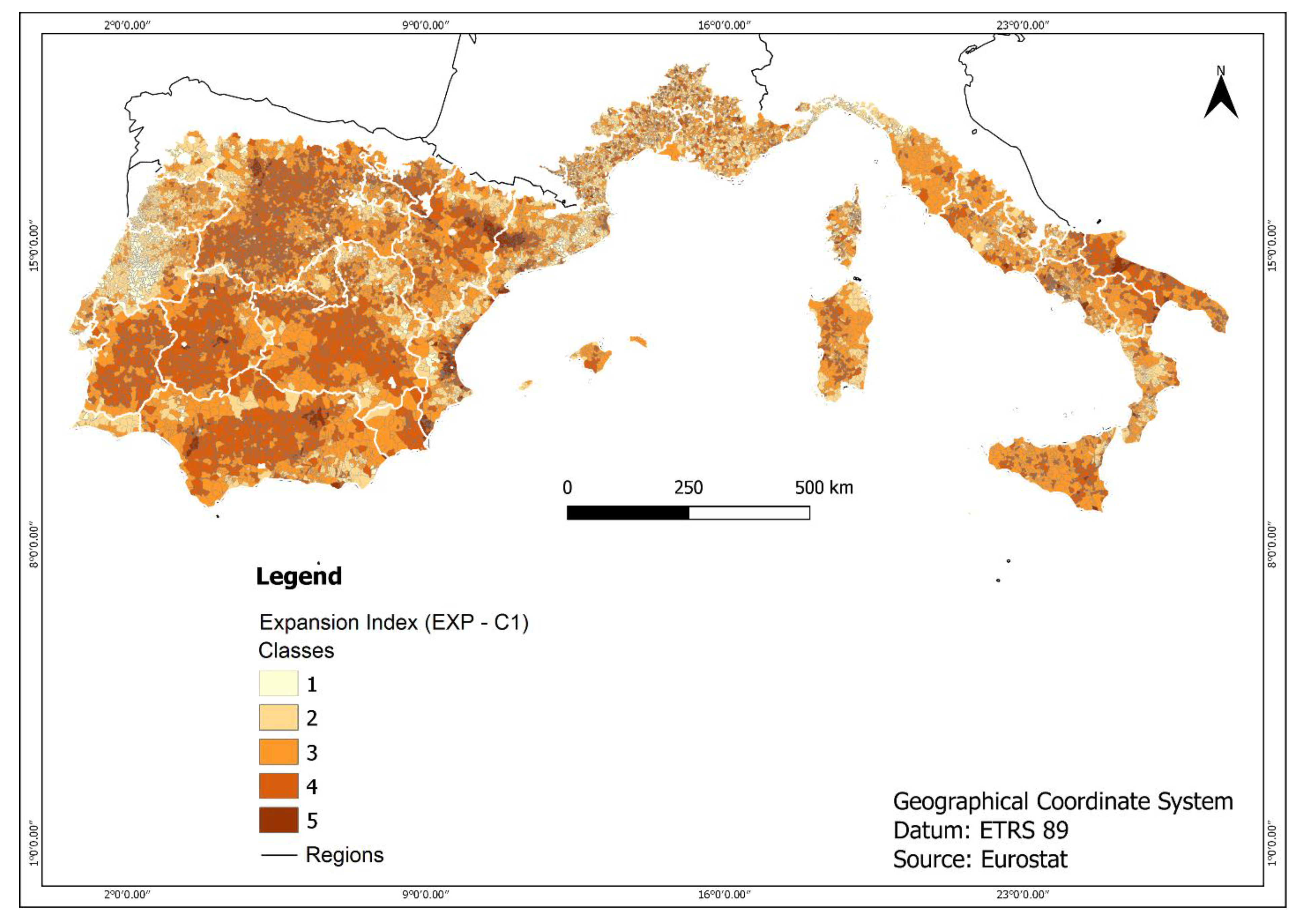
In C1, the distribution of the EXP index does not show a macroscopic trend relatable to the geographical (internal or coastal areas) or political (countries of origin) conditions (Figure 9). Generally, we can observe a negative correlation between the EXP values and the LAUs characterized by high demographic conditions noticeable in the touristic (i.e., the Costa Smeralda in Sardegna—IT and the Côte d’Azur in France) or in metropolitan areas (i.e., Roma, Barcelona or Madrid).

Excluding these local interactions, it is difficult to identify a general gradient even if some spatial aggregations are evident.

For instance, many LAUs with EXP = 4 are concentrated in some portion of Castilla y Leon, Andalucía, Extremadura and Castilla La Mancha (ES), Alantejo (PT) and, to a lesser extent, in Provence Alpes Côte D’Azur (FR), or in Puglia and Basilicata (IT).

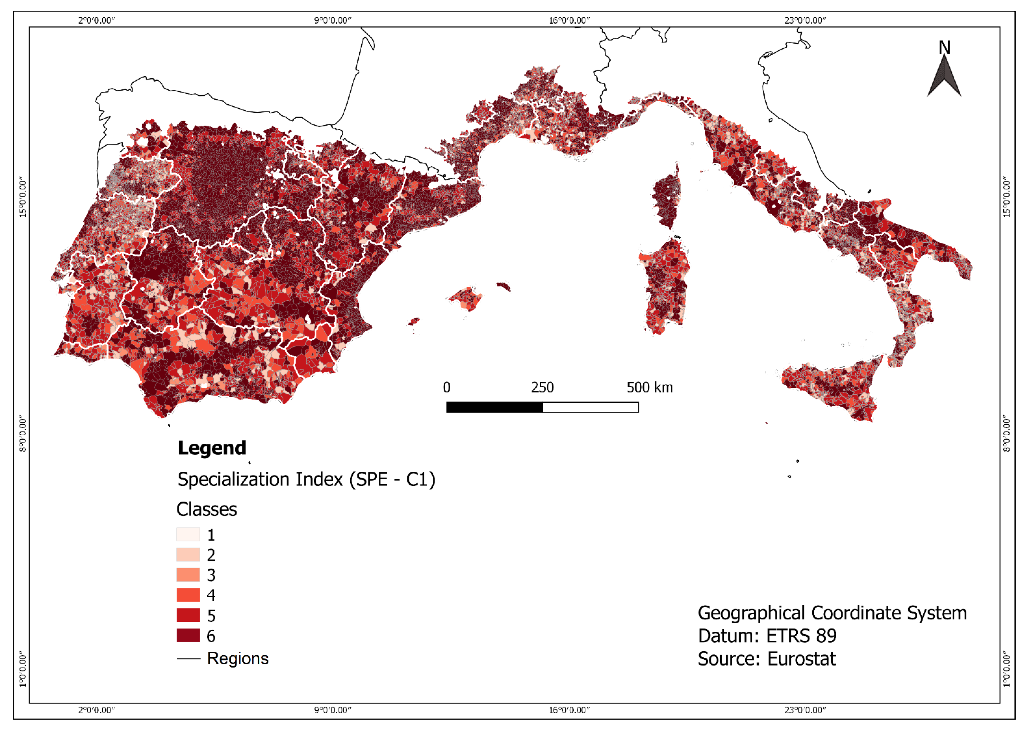
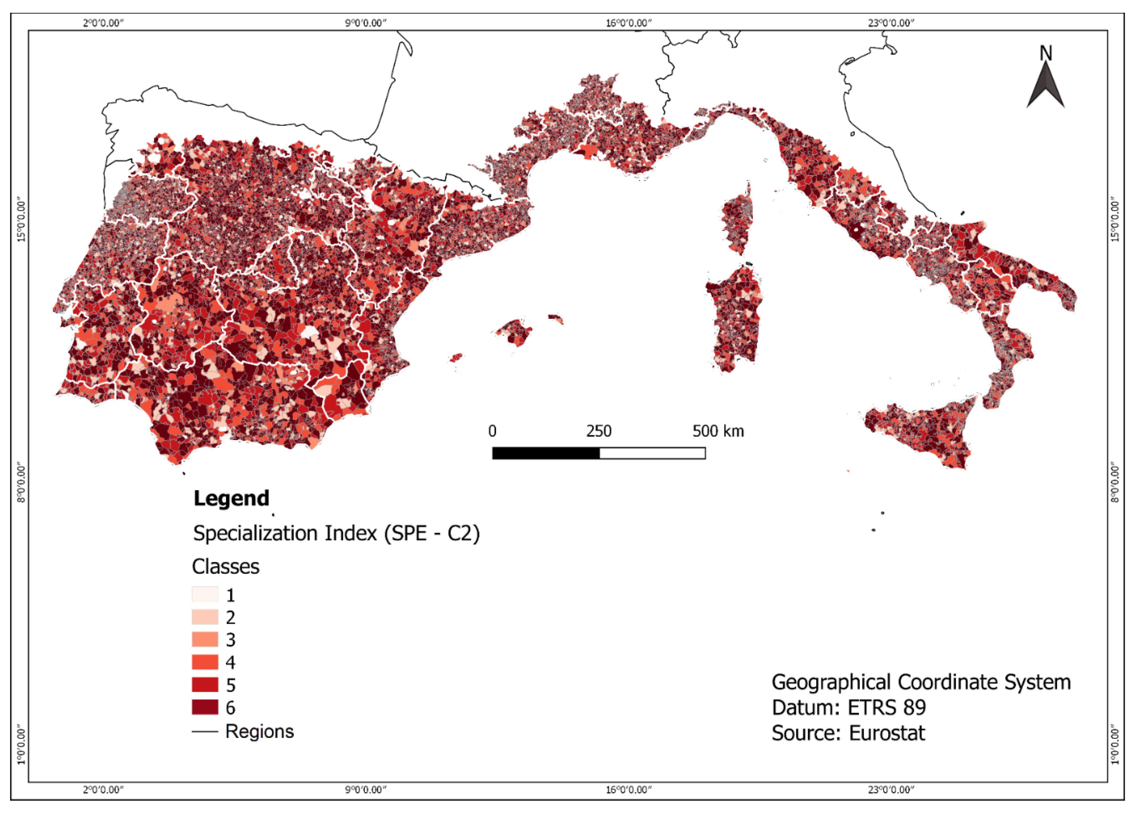
The spatial pattern of the SPE in C1 seems to be partially correlated to the EXP index distribution (Castilla y Leon and Andalucía) and locally affected by the proximity of LAUs to touristic areas (Figure 10).

For instance, an area of highly specialized agricultural systems (SPE = 6) is identifiable along the Eastern coasts of Spain, in much of the Castylla y León and Andalucía (ES), or in the Western coast of Corsica (FR), Toscana and Lazio (IT). The reason can be that the farmer’s decisions about the crop choice are driven by the environmental conditions (soil nature and climate), which can affect also the intensification in land use, or by the local demand for food linked to displacement of people due to recreational purposes.

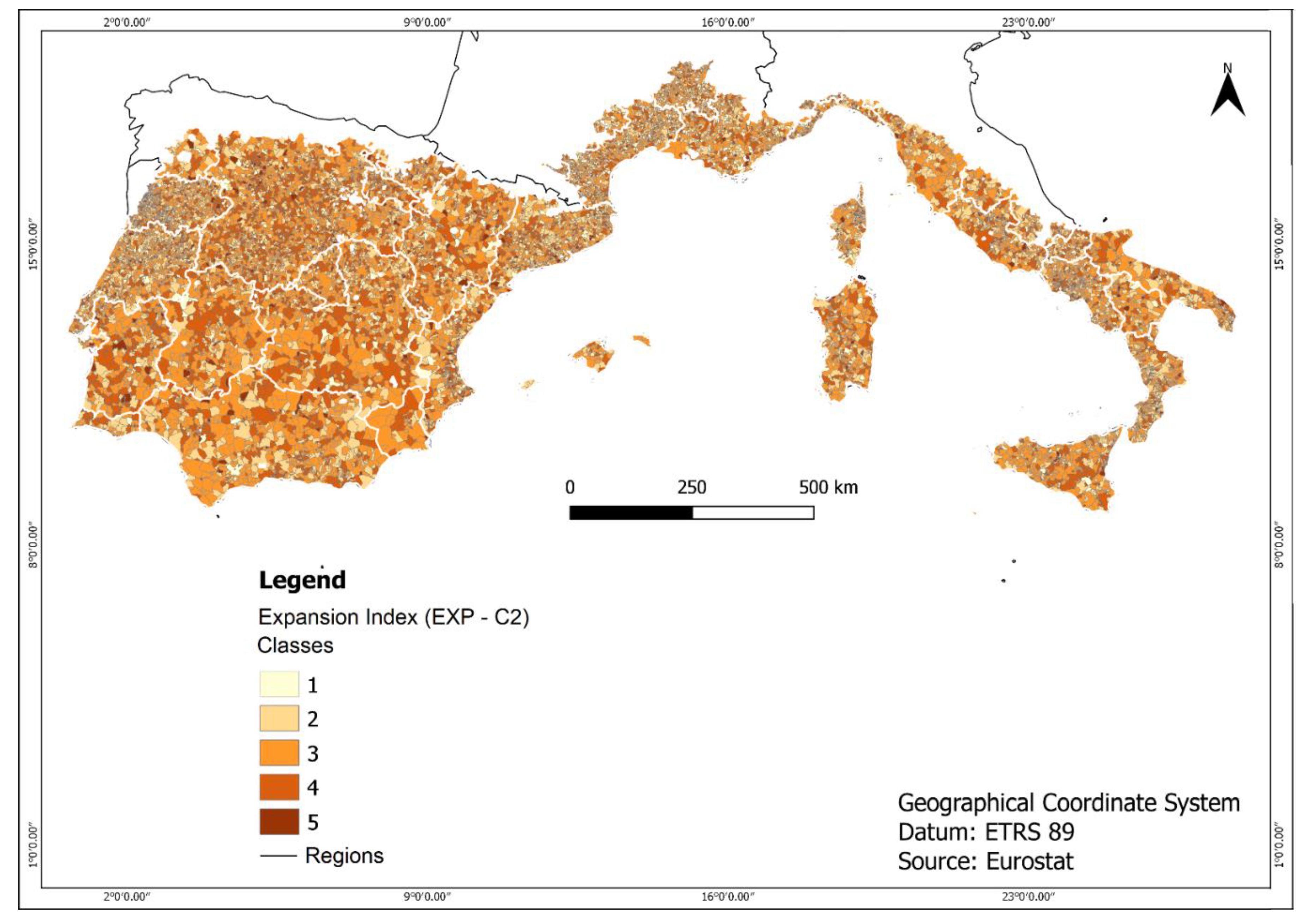
The comparison with C2 highlights an evident fragmentation of the spatial clustering of LAUs that was previously observed. Both for EXP and SPE, the pictures of the study areas (Figure 11 and Figure 12) reported a dense mosaic of different patches that made aleatory the research of any relationships. The only regions that escaped partially this trend were the southern part of Portugal (Algarve and Alantejo) and Spain (Andalucía, Extremadura and Castilla La Mancha, Région de Murcha) and some portions of Italian regions (Toscana, Puglia, Sicilia and Sardegna).

On a more general level, the trends towards a reduction of specialization and, to a lesser extent, land-use intensity of agricultural systems are evident. It is worth to note that in some limited areas where the intensification level in land use was very low (EXP = 1), we note a turnaround as in Norte, Centro and Algarve (PT), or Provence Alpes Côte D’Azur and Corsica (FR), Cataluña (ES) and Liguria (IT).

4. Discussion

The first result emerging from the comparative analysis of the two last census data was the decrease of surface devoted to agricultural use. The reduction of TFA, UAA, AL, PC and PG were all signs pointing out a progressive discouragement of farmers that found a confirmation also in the corresponding increase of RS, largely characterized by a less professional activity and the competition in land use exerted by urbanization. These results are in agreement with most of the recent literature about Mediterranean agricultural dynamics, both at a global and local scale [1,28,29]. In fact, the progressive decrease on cultivated surface could be the results of abandonment of most marginal areas [30,31] or the urbanization of the cultivated regions, such as the fertile coastal areas [32] and the most populated peri-urban ones [33].

On the other hand, the increase of IA seemed to highlight the existence also of an opposite strategy based on the adoption of more intensive farming practices, although it was significantly smaller in size. Additionally, in this case, we can find confirmation of this result in the recent literature, highlighting the two opposite dynamics occurring on Mediterranean land systems: farming extensification and abandonment on one side, and the intensification of cultivation methods on the most fertile areas [34,35].

Another point concerns the fragmentation of AT recorded during this 10-years span as the increasing number of identified ATs and reduction of their incidence in terms both of LAUs and hectares involved. In Mediterranean countries, fragmentation can derive from different processes, such as land inheritance and transmission systems [36], traditional smallholder farming [37] and urbanization dynamics [38]. This process could impact the decision-making process of farmers [39] and also the sustainability of agricultural production [40]. Moreover, an increasing fragmentation means greater uncertainty about how to manage agricultural systems and a decreasing efficacy of the most traditional models from an economic and agronomic point of view. In this sense, it assumes a particular relevance the trend observed on mixed (i.e., non-specialized) agricultural systems, which decreased in their diffusion comparing to the other ATs, but increased in terms of both LAUs and overall area. Indeed, the specialized agricultural systems, while remaining the most widespread, reduced significantly their presence.

The overall picture resulted by the analysis of data coming from the first analyzed agricultural censuses (C1) was an agriculture still well rooted on land and quite specialized. These two important elements of agricultural systems (intensification and specialization), whose behavior was described by EXP and SPE indices, seem to be differently distributed among the LAUs of Western Mediterranean area. EXP drew a bell-shape curve of distribution that revealed the existence of an ordinary level of intensity in the use of land and water within the study area, whereas SPE highlighted the need for farmers to move towards specialized productions. As stated before, the evaluation of intensification based only on census data is largely incomplete since it considers only the use of land and water by neglecting other inputs to agricultural systems (machinery, agro-chemicals, genetics and changes in farmers’ skills). However, above all UAA and AI can be considered as a proxy for cares given in agricultural practices and, to some extent, they are positively correlated with the use of inputs.

EXP and SPE were substantially independent between them, with the only partial exception regarding the tendency of a higher intensity in land-use for the most specialized agricultural systems. Therefore, we found the same pattern of the EXP classes within each class of SPE and likewise the same tendency towards specialization within each class of EXP. This could mean that farmers deal with separately the two questions “what to grow?” and “how to grow?”, despite what is suggested by modern agronomy with the definition of cropping and farming systems [41].

About the changes occurred over the 10-years span (C2), we observed that the choices made in terms of UAA composition (AL, PC, PG and RS) resulted in being more dynamic than those concerning the use of land and water factors. For farmers it was easier to change the productive strategy of farm (i.e., cultivating different crops), rather than modify the whole farming system, in terms of size of farms (TFA) or the portion of cultivated area (UAA) or again the irrigated surface (IA). Certainly, the driving-forces acting on these factors were completely different: (i) the competitive use of land and the loss of profitability of agricultural activity for TFA and UAA; (ii) the investment availability of farmers and the climate changes for IA and (iii) the trend of commodities prizes at the worldwide level, the CAP and the changes in eating habits for AL, PWC, PFC and RS. The general tendency seems to be toward a reduction of both intensification and specialization even if with a different rate of variation (higher for specialization, lower for intensification).

The incidence of most specialized agricultural systems (SPE = 5 and 6) decreased and that of the most intensive ones remained constant (EXP = 5), whereas the reduction of LAUs for the agricultural systems belonging to the previous class (EXP = 4) was significant. Mixed agricultural systems (SPE = 2 or 4) with a moderate level of land-use (EXP = 2 or 3) grew more clearly, but this trend appeared to be the result of the crumbling of the specialized agricultural systems rather than the adoption of more diversified productive strategies by farmers. In any case, the dynamics, which involved the two indices, occurred independently from each other. This means that the LAUs passing from a class of SPE to another followed the same pattern of distribution through the class of EXP and vice versa.

Finally, from a spatial point of view it is clear that the traditional agricultural districts still well evident in C1 are crumbling under the pressure of different and unexpected driving-forces highlighting how farmers choose different strategies to deal with the changes. In some regions characterized by a low level of land use, we observed also a turnaround that confirms the lack of effective and generalizable responses to the problems posed by the crisis conditions.

Among the many possible food for thoughts, some are worthy of being deepened. The different evolution of TFA and UAA over time was partially the effect of a re-organization at farm level that, under the pressure of a reduction in agricultural land-use, implied a higher level of cultivation of available land. However, this process has occurred at the expense of the PG, whose conservation is a goal of the current CAP, and to advantage of RS, which are the sign of a progressive disengagement of farmers. The importance of PG in carbon sequestration, erosion control and biodiversity conservation make the environmental reading of this result definitely worrying.

The country does not seem to affect the agricultural systems distribution. This convergence of behavior is probably the results of many driving forces that, acting at more local level, are very difficult to interpret.

5. Conclusions

In this paper, we analyzed the existing agricultural systems and their dynamics on the Western Mediterranean countries, starting from the two last national agricultural censuses at the most detailed scale available. We developed two indexes, in order to understand the processes of intensification in land-use and specialization in land-cover occurred on the ten years’ time span. Even if the range of time was short for a global analysis, we identified different interesting trends, which could be confirmed with the next census expected on 2021.

First of all, we observed a general decrease of cultivated areas, a trend throughout abandonment that occurred both on the more populated and on the most marginal regions, highlighting the two underlying processes: urbanization on one side and abandonment of the more extensive traditional agricultural activities. Moreover, a fragmentation of the agricultural landscape mosaic has been observed. This was proved by the frequency decrease of the specialized agricultural systems compared to the mixed ones passing from C1 to C2. At the same time, we observed a discouragement in the agricultural use of land and in its cultivation. The irrigated surfaces were the only intensity indicator that have increased, although to a lesser extent than we expected, as an adaptation to climate change increasing temperature/evapotranspiration on the region.

The answers of farmers to changed environmental and economic conditions seemed to consist of a more diversified production (probably to limit the risk from the market instability) and a shrinkage of agricultural and cultivated land under the pressure of competitive soil uses and decreasing prices of agricultural products. We noted that the agricultural systems most intensive in land-use (EXP = 5th class) survived substantially unchanged over time, whereas the main reduction was recorded for the agricultural systems belonging to the immediately preceding class (probably because the productivity of those areas do not justify such a use of land factor).

It is possible that these processes, which started in 2010, are already today even more developed than we described. For this reason, an interesting future development of this study will be to analyze how the European policies played a role on the mentioned dynamics.

At the same time, a future analysis could be devoted to understand the trajectories drawn by LAUs in a more detailed form with the aim to bring out the effects attributable to both the geographical position and the starting agricultural system typology on the process of changing.