Article

Early Detection of Broad-Leaved and Grass Weeds in Wide Row Crops Using Artificial Neural Networks and UAV Imagery

by
Jorge Torres-Sánchez
1,*,
Francisco Javier Mesas-Carrascosa
2,
Francisco M. Jiménez-Brenes
1,
Ana I. de Castro
1,† and
Francisca López-Granados
1
1
Grupo Imaping, Instituto de Agricultura Sostenible-CSIC, Avda. Menéndez Pidal s/n, 14004 Cordoba, Spain
2
Department of Graphic Engineering and Geomatics, Campus de Rabanales, University of Cordoba, 14071 Cordoba, Spain
*
Author to whom correspondence should be addressed.
Current address: Weed Control Group, Plant Protection Department, National Agricultural and Food Research and Technology Institute-INIA, Crta. de la Coruña, km 7,5, 28040 Madrid, Spain.
Agronomy 2021, 11(4), 749; https://doi.org/10.3390/agronomy11040749
Submission received: 3 March 2021 / Revised: 8 April 2021 / Accepted: 10 April 2021 / Published: 12 April 2021

Abstract

:
Significant advances in weed mapping from unmanned aerial platforms have been achieved in recent years. The detection of weed location has made possible the generation of site specific weed treatments to reduce the use of herbicides according to weed cover maps. However, the characterization of weed infestations should not be limited to the location of weed stands, but should also be able to distinguish the types of weeds to allow the best possible choice of herbicide treatment to be applied. A first step in this direction should be the discrimination between broad-leaved (dicotyledonous) and grass (monocotyledonous) weeds. Considering the advances in weed detection based on images acquired by unmanned aerial vehicles, and the ability of neural networks to solve hard classification problems in remote sensing, these technologies have been merged in this study with the aim of exploring their potential for broadleaf and grass weed detection in wide-row herbaceous crops such as sunflower and cotton. Overall accuracies of around 80% were obtained in both crops, with user accuracy for broad-leaved and grass weeds around 75% and 65%, respectively. These results confirm the potential of the presented combination of technologies for improving the characterization of different weed infestations, which would allow the generation of timely and adequate herbicide treatment maps according to groups of weeds.

1. Introduction

Weeds are one of the main causes of crop losses in arable crops worldwide [1]. Traditionally, their control has been addressed through the application of herbicides to the entire crop field without taking into account that weeds usually have a patchy distribution and there are weed-free areas [2,3,4,5]. This has led to excessive consumption of herbicides which causes economic consequences and environmental concerns. To decrease both problems, there is a set of guidelines reported in European legislation addressing the Sustainable Use of Pesticides [6,7] which are compatible with the use of site-specific weed management (SSWM) techniques that allow the design and application of herbicide treatments that target only the areas where weeds proliferate. One of the key components of SSWM is the aim of providing accurate and timely early weed control based on weed infestation maps obtained by proximal (ground) or remote sensing [8].
In recent years there have been major advances in weed detection and different novel technologies have been developed that make it possible to detect weeds in the early post-emergence stage from both ground and aerial platforms by means of computerized processing of data [9]. One of the most widely used platforms with the greatest potential for installing sensors for early weed detection has been unmanned aerial vehicles (UAVs) [9,10,11,12]. This is because UAVs have significant advantages over other remote platforms, such as the possibility of flying at low altitudes, providing very high spatial resolution imagery (less than 1 cm per pixel [13]), flying under clouds, using a wide spectral and size range of embedded sensors, and providing the option of obtaining images on demand at almost any time. In comparison with on-ground platforms, the main advantages are that the use of UAVs is less expensive and does not cause soil compaction, and they can fly to muddy or difficult to access areas [14]. Therefore, the analysis of UAV imagery has allowed the generation of localised treatment maps through which it is possible to greatly reduce the area treated in the fields and, consequently, the consumption of herbicides [15]. López-Granados et al. [16] studied different weed management scenarios based on weed threshold, which is the weed infestation level above which a treatment is required, as the baseline to generate herbicide treatment maps, achieving herbicide savings higher than 70%.
An ideal characterization of weed infestations should not be limited to the spatial identification of weed stands. It must also be able to perform an early discrimination between the types of weeds growing in the crop field in order to allow the best possible choice in the type of herbicide treatment to be applied and to avoid the use of a wide spectrum herbicide. A first step in this direction should be the separation between weeds into the two main groups: broad-leaved and grass weeds. This is a major challenge because crop plants, grass and broad-leaved weeds show a parallel phenological stage at early growth phases, as well as similar spectra and appearances. The detection of weeds using images taken by UAVs has been approached in different ways.
One of the most common methodologies for UAV-based weed detection is built on the assumption that plants growing outside the crop line are weeds, so algorithms have been developed that first detect the vegetation, and then delineate the crop lines and classify the plants growing outside the lines as weeds [15,17,18]. Other works have focused on detecting weeds by analyzing their spectral properties [19,20]. There has also been work to make it possible to detect weeds not only between (outside) but also within the crop lines, by combining the detection of crop lines with the use of automatic learning methods [21,22,23]. In a large number of these studies there has been a trend towards segmenting the image into objects. These objects are groups of homogeneous pixels which, in the analysis of very high-resolution spatial images, allow a reduction in the heterogeneity of the classes to be detected, and allow contextual and spatial information to be added to the spectral information contained in the raw UAV images. Therefore, it can be said that these works are framed in the analysis paradigm known as object-oriented image analysis (OBIA), in such way that the basic information unit for image classification is based on objects, not on pixels [24].
Artificial neural networks (ANNs) are widely used methodologies in remote sensing for the resolution of complicated classification problems [25,26]. One of the main characteristics of this type of model is its learning capacity. A standard neural network consists of many processors called neurons that are connected to each other [27]. The input neurons are activated by the information provided by the user, and when activated, they process this information and communicate it to the following neurons, thus reaching the desired result, which, in the case of remote sensing, is the classification of an image. The assignment of weights and relationships between the neurons is produced by means of automatic learning, carried out on a set of samples that are introduced as training in the design of the model. One of the most widely used types of neural networks in remote sensing is the multilayer perceptron (MLP) neural network [28] which has been successfully used in high-resolution satellite imagery for weed detection [29]. In MLP, neurons are organised into three or more layers. First, there is an input layer containing the information from the samples to be analyzed, followed by one or more hidden layers, and finally there is the output layer that produces the desired result.
Discrimination between broad-leaved and grass weeds has been addressed previously by using images taken on the ground or by ultrasonic sensors mounted in front of a tractor [30,31]. However, to our knowledge, this is the first time that the early detection of different groups of weeds in crop fields has been attempted using UAV imagery. Therefore, the aim of this paper is to explore the potential of combining images from UAV, and OBIA and MLP ANN techniques for discriminating between broad-leaved and grass weeds in broad-leaved wide-row crops.

2. Materials and Methods

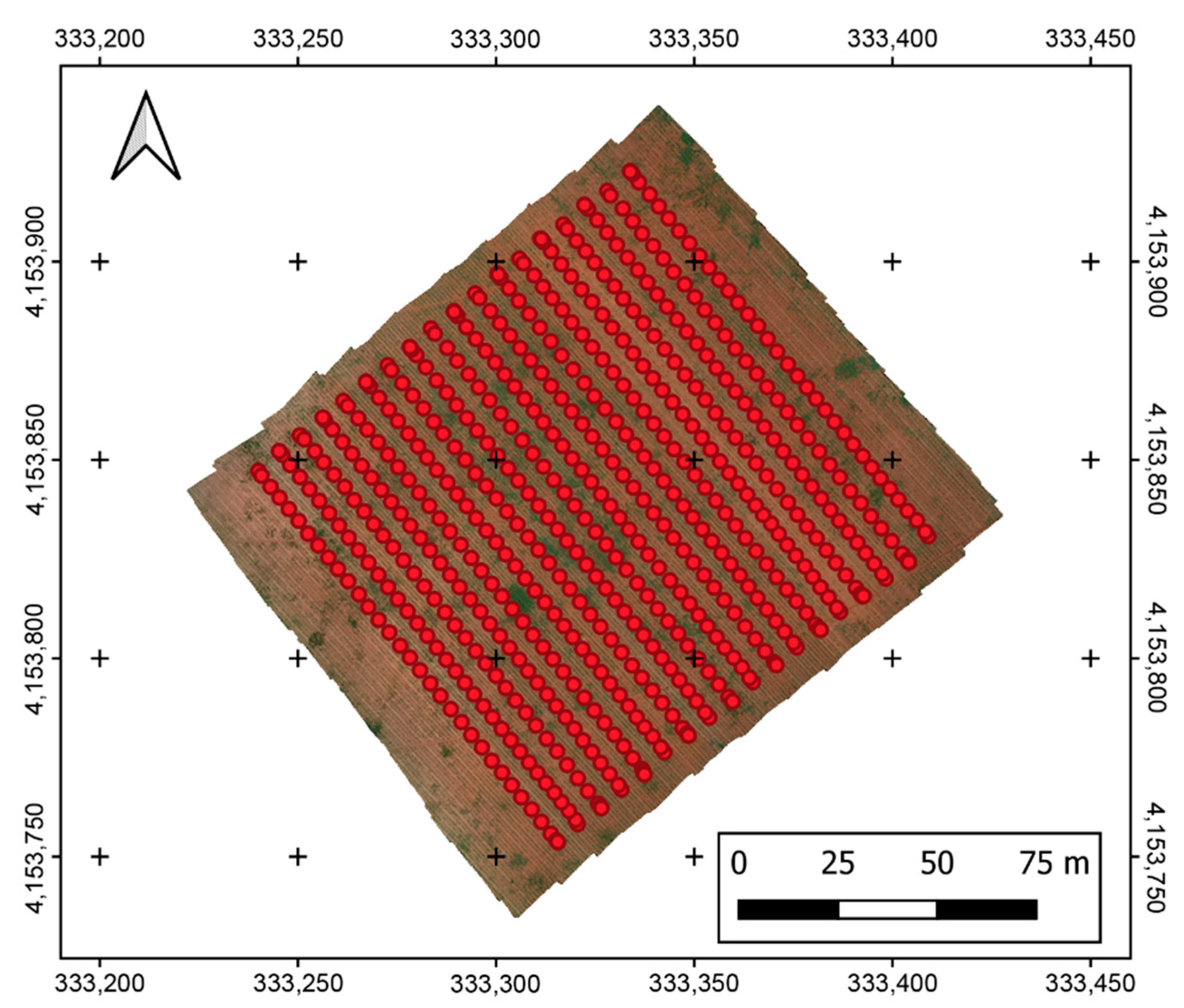
2.1. Description of Study Fields and UAV Flights

This study was performed on two different wide-row crops, sunflower and cotton, selecting one field for each crop. Table 1 shows the information related to inter-row spacing in meters, as well as the location and area in hectares for both fields, being sunflower and cotton crops under rainfed and irrigation conditions, respectively. The fieldwork phase was carried out approximately 3 weeks after sowing. At this stage, both crops had an average height of 15–20 cm approximately (Figure 1) and were naturally infested by different broad-leaved and grass weed species, with the cotton field showing a higher level of weed infestation. A wider variety of broad-leaved than grass weed species was identified in both crops (Table 2).
A UAV quadcopter model MD4-1000 (microdrones GmbH, Siegen, Germany) was used as an aerial platform to acquire images. This UAV, with vertical take-off and landing, is battery powered and can be manually operated by radio control or autonomously by means of its global positioning system (GPS) receiver and its waypoint navigation system. A visible-light (RGB: red (R), green (G) and blue (B)) low-cost camera model from Sony ILCE-6000 (Sony Corporation, Tokyo, Japan) was attached to the UAV in order to capture the images. This camera was composed of a 23.5 × 15.6 mm APS-C CMOS sensor capable of acquiring 24 megapixels (6000 × 4000 pixels).
A UAV flight for each crop was carried out at the beginning and at the end of May for the sunflower and cotton fields, respectively. The UAV route was adjusted to fly at a 20 m altitude with a forward and side overlaps of 74% and 70%, respectively (Figure 2). The flights were carried out at noon to take advantage of the sun’s position and thus minimize shadows on images. The UAV flight and sensor configuration led to a spatial resolution of around 4 mm, which met the requirement of being lower than 10 mm for RGB sensors, established previously in a review about weed detection using UAV imagery [9].

2.2. Digital Surface Model (DSM) and Orthomosaic Generation

Once the UAV images were acquired for both crops, Agisoft PhotoScan Professional Edition software, version 1.2.4 build 2399 (Agisoft LLC, St. Petersburg, Russia), was used for generating the geomatic products. First, a three-dimensional (3D) point cloud was created by applying the structure-from-motion (SfM) technique. Then, a digital surface model (DSM) was generated from the previous 3D point cloud, which provided height information. The final product was an orthomosaic of the whole fields, in which every pixel contained RGB information as well as spatial information (Figure 3).
All geomatic products were created automatically. However, the manual localization of six ground control points (GCPs) [32,33] was necessary, with four placed in the corners and two in the center of each field, in order to georeference the geomatic products. The GCP coordinates were measured using two GNSS receivers: one was a reference station from the GNSS RAP network from the Institute for Statistics and Cartography of Andalusia (Spain), and the other one was a GPS with one centimeter accuracy, used as a rover receiver (model Trimble R4, Trimble company, Sunnyvale, CA, USA). At the beginning of the image processing, the software matched the camera position and common points for every image, which allowed the refinement of the camera calibration parameters. More information about the PhotoScan functions can be found in [34].

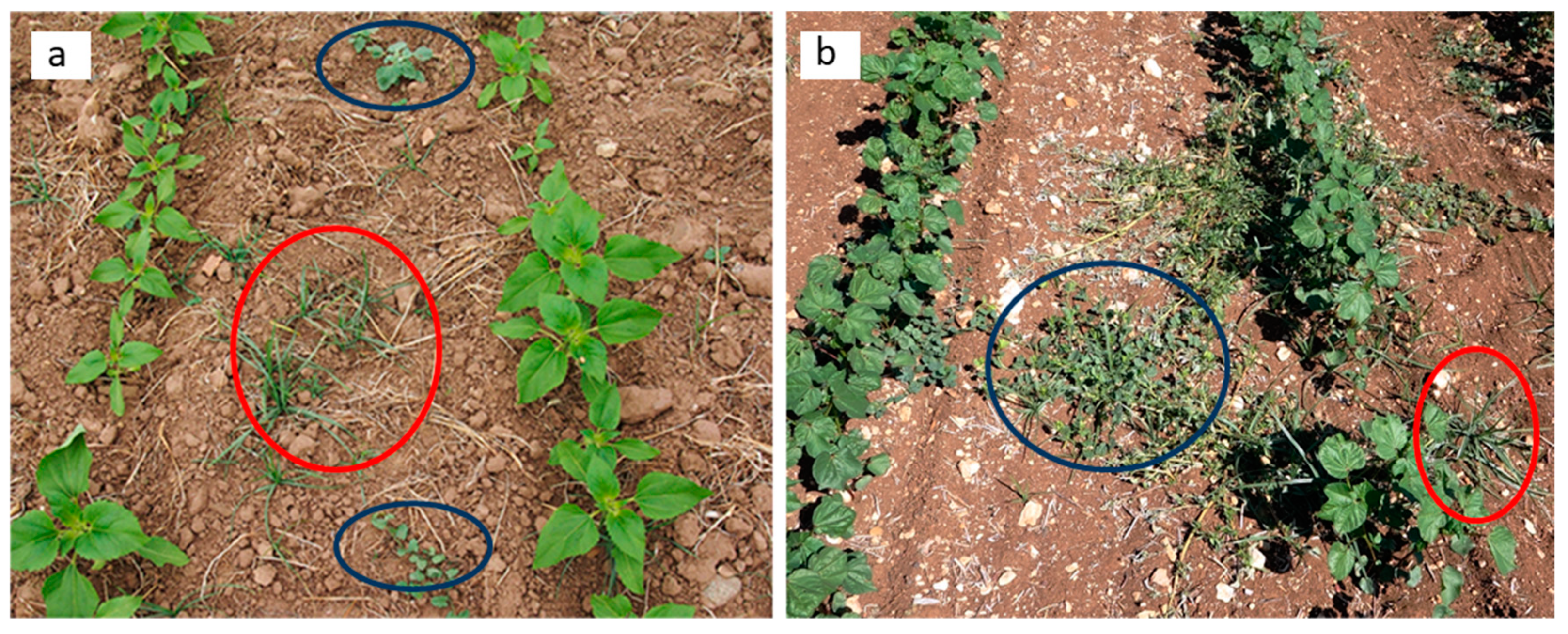
2.3. Ground Truth Data
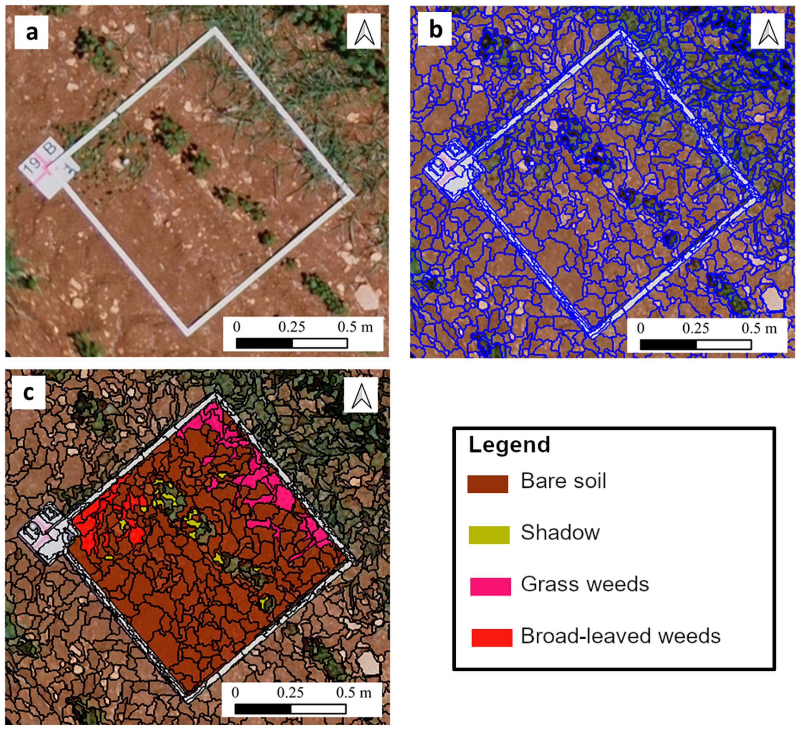
A total of 30 georeferenced sampling 1 × 1 m white frames were placed in both crops. These frames contained either broad-leaved, grass weeds, or both of them. Their placing ensured that sunflower and cotton fields had an equal chance of being sampled without operator bias [35]. After each frame was placed in every field, it was manually photographed by a conventional camera perpendicular to the ground. These photos were later used for ground truth data when carrying out the manual classification on orthomosaics in the image analysis phase, detailed in the following section.

2.4. Image Analysis

The workflow developed in the image analysis procedure is summarized in Figure 4. The following sections explain the details of each of the steps of this workflow.

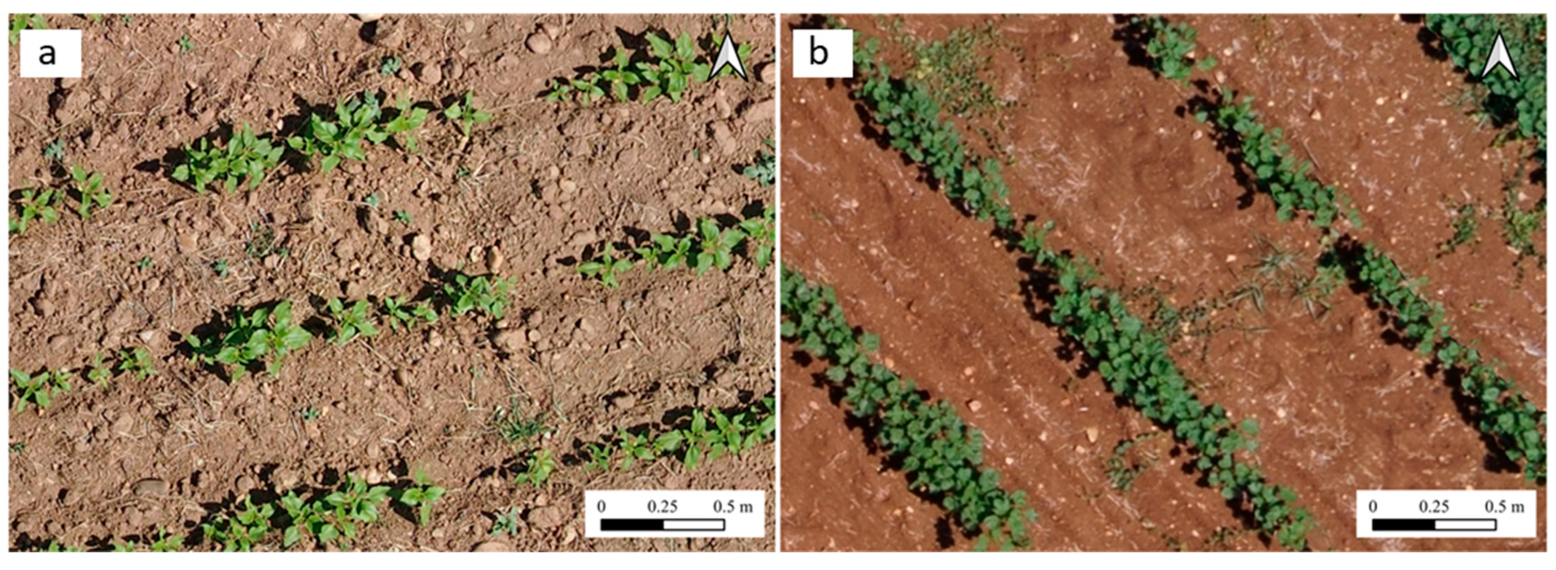
2.4.1. Labeling of the Image Objects

The first step in the development of the image analysis procedure was the segmentation of the image in objects formed by adjacent and spectrally homogenous pixels according to a procedure known as segmentation. In this work, the multiresolution segmentation algorithm (MRSA) [36] was carried out using eCognition Developer 9 software (Trimble GeoSpatial, Munich, Germany). This algorithm is controlled by a set of parameters that must be fixed by the user: scale parameter, colour/shape weights, and smoothness/compactness weights. The first parameter controls the homogeneity of the pixels included in the objects and is related to their final size (more homogeneous objects lead to smaller sizes). The colour/shape weighting determines if the segmentation pays more attention to the spectral information or to the shape of the objects. The last parameter controls if the creation of the object is spatially compact or if it is dominated by the spectral homogeneity (smoothness). Based on previous experience in the optimization of UAV imagery segmentation for vegetation detection [17,22,37] and on some internal tests, the values of the parameters were: 15 for the scale parameter, 0.6/0.4 for colour/shape, and 0.5/0.5 for smoothness/compactness.
After the image segmentation, the results of which can be viewed in Figure 5b, the next step was the manual labeling of the objects inside the reference white frames that were laid on the fields as explained in Section 2.3. In this part of the workflow, objects were divided into the following classes: bare soil, shadow, broad-leaved weeds, and grass weeds. The high resolution of the UAV imagery (4 mm as stated before) allowed discernment between the classes and, in the case of doubt, the field photographs of the reference frames were used to help in the disambiguation process. This step was carried out by only one expert in order to avoid discrepancies in the manual labeling of the samples that were used in the generation of the neural network. Figure 5c shows one of the reference frames after the labeling of the image objects.
The total number of labeled objects is shown in Table 3. Due to the early stage of the crop development, the class with the highest representation in the datasets was bare soil in both studied crops. The amount of objects labeled as weeds depended on the natural weed infestation level of the crops. The cotton field suffered a more intense infestation and, consequently, it presented a higher number of objects labeled as weeds. In order to feed the neural network with a balanced dataset, the number of labelled objects for each class was reduced to match the number of objects of the class with lower representation. Consequently, as the class with the fewest objects in the sunflower field was broad-leaved weeds with 635 objects, 635 samples from each class were randomly selected to match the number of broad-leaved weed objects. In the cotton field, the final number of objects in each class was 421, to match the number of grass weed objects, which was the least represented class in the training dataset.
A set of 49 features (Table 4) was extracted from the labeled objects to feed the neural network. The extracted features were divided into three main categories: spectral, geometric, and textural. The first one was related with the spectral values extracted from the three channels of the RGB sensor and included normalized band values, some of their statistics, and a set of vegetation indices. The geometric features were related with the shape of the objects created by the MRSA, and also included the height of the objects above the soil. The textural features explained the variation of the spectral values inside the objects, and included variables related to the gray level co-occurrence matrix (GLCM), which is a tabulation of how often different combinations of pixel gray levels occur inside an object [38]. Among the textural features, there were also variables related to the gray level difference vector (GLDV) [39], i.e., the sum of the diagonals of the GLCM.

2.4.2. Crop Detection

The first step after the manual labeling of the input for the neural network was the automatic detection of the objects belonging to the crop rows. In this step, an automatic OBIA algorithm previously developed and fully validated [15,17,22] was used. This algorithm detects the vegetation (crop and weeds) by applying a thresholding methodology to the ExG values of the segmented objects. Then, the algorithm splits the image into strips and, through an iterative process, searches for the orientation of the strips that best fits the distribution of the vegetation objects in the image. When this orientation is calculated and, taking into account the distance between the crop rows, the algorithm splits the image into strips representing the crop rows, and all the vegetation objects below these strips are classified as crop. More details about the algorithm can be found in the above referenced works.

2.4.3. Artificial Neural Network Creation

Once the crop objects were classified using the automatic OBIA algorithm, the remaining objects were classified as “soil”, “shadow”, “broad-leaved weed”, or “grass weed”, using a neural network. The feature values from the manually labeled objects were used for training and validating an MLP neural network in IBM SPSS Statistics software (IBM Corp. Released Version 26.0. Armonk, NY, USA). Of the total manually labeled objects, 60% were used to train the neural network, 20% were used as a test set to track errors during the training and to avoid overfitting [52], and the remaining 20% were reserved to validate the accuracy of the neural network. The size of the MLP neural network is defined as the size of the input layer × the size of the hidden layer × the size of the output layer. In the parameterization of the neural network generation, the input layer was formed by the 49 extracted object features, the output layer contained 4 neurons, corresponding to the 4 classes sought, and SPSS was configured to optimize the number of neurons in the hidden layer in a range between 1 and 50. Batch training was used in the generation of the neural network. This method updates the synaptic weights of the neurons when all the training data have been passed. The optimization algorithm applied in the batch training was the scaled conjugate gradient, a fully automatic algorithm that does not require the input of parameters by the user [53].

2.5. Validation

The performance of the MLP neural network was assessed using the confusion matrix [54], created from the validation datasets in both crops. Based on the confusion matrix, the overall accuracy (percentage of pixels correctly classified) was calculated, as well as the user’s (or commission error indicating the percentage of pixels classified as a class that should have been classified as a different class) and the producer’s accuracy (or omission error indicating the proportion of pixels from a class that were misclassified as a different class) for the four classes assigned by the neural network: soil, shadow, broad-leaved weed, and grass weed.

3. Results and Discussion

The optimization process of the hidden layer carried out by the software in the development of the neural network led to this layer having eight neurons for cotton and sunflower crops. Table 5 and Table 6 show the classification results in each of the sample subsets for sunflower and cotton, respectively. The overall accuracy for the sunflower field was 83.64%, whereas for cotton it was slightly lower, at 78.16%. In both cases the accuracy was around 80%, so it can be said that satisfactory accuracies were obtained. The final accuracies achieved in the validation data set were similar to those obtained in the training and test subsets, where values in the range of 80% were also obtained.
Analyzing Table 5 and Table 6 in detail, it can be seen that the highest accuracies were obtained in the detection of soil and shadow, whereas the classes among which there was most confusion were the different types of weeds. However, taking into account the difficulty of the task and the similarity of broad-leaved and grass weed classes, the classification of both groups of weeds was good. Observing the producer’s accuracy, it can be seen that around 75% of the broad-leaved and grass weeds in the sunflower field were correctly classified; meaning that some pixels of the broad-leaved and grass weeds were not identified and thus the procedure underestimated the total area of every weed patch. From the point of view of the user of the classification, 78.81% of the objects classified as broad-leaved weeds actually belonged to this class. According to these results, a treatment map based on the neural network would therefore allow broad-leaved weeds to be specifically treated with a high level of precision. This precision would be less for grass weeds, since, analyzing the user’s accuracy, it could be seen that 67.46% of the objects classified as this type of weed actually corresponded to this type of vegetation. From an agronomic point of view, it would be desirable to consider that the producer’s accuracy would be lower and the user’s would tend to be higher, thus weed patches would be less likely to be missed, taking into account the likelihood that farmers would choose to treat weed-free zones rather than assume the risk of allowing weeds to go untreated [55].
In the cotton field the results of the user’s accuracy for weeds were very similar to those obtained for the sunflower field. Consequently, the accuracy of a possible treatment map in the cotton field would also be higher for broad-leaved weeds. The fact that the accuracies obtained for the sunflower crop were slightly higher could be linked to the fact that in this crop the variability of weed species was lower (Table 2). Therefore, in the creation of the neural network the group of weed training samples had a higher homogeneity and it was easier for the software to calculate a group of parameters that distinguished broad-leaved from grass weeds. This is in agreement with Lottes et al. [56] who created a classification scheme to discriminate saltbush and chamomile from “other weeds” in a sugar beet field using UAV imagery, and they also reported the heterogeneity of the class “other weeds” as one of the plausible reasons for this class having lower accuracy in their classification.
Table 7 and Table 8 show the 10 most important variables in the creation of the neural network for sunflower and cotton, respectively. Complete tables including the importance of all variables can be consulted in Appendix A. In both crops, brightness was the most important variable, which is probably related to the excellent discrimination of shadows from the rest of the classes in the classification. In the sunflower field, and without counting brightness, seven of the most important variables were spectral, including HUE, the normalized red band and several vegetation indices. Among these most important variables, there was only one of a textural type, the GLDV entropy. For cotton the situation was different, as of the 10 most important variables five were of a textural type, most of them related to GLCM. This importance of using textural features for weed classification using UAV imagery has been previously reported in the scientific literature [9,23,57].
It is also noteworthy that in the sunflower crop the height of the objects above the ground was chosen among the most important variables, which could indicate that the weeds in this field showed a more erect bearing than in cotton, and therefore that the height was a determining factor in the classification. The importance of height in weed discrimination was also reported by Zisi et al. [57], whose results improved when including this feature in their analysis. In the neuronal network for the sunflower crop, the 10 most important variables had values of standardized importance higher than 70%, whereas in the case of cotton, only the brightness presented an importance higher than 70% whereas the others had much lower importance, that being between 66% and 49%. This could indicate that in the case of sunflowers, more variables were important for the correct classification of objects, whereas in the case of cotton fewer variables were relevant. A feature selection procedure was not carried out in our study since some authors [21] reported that feature selection was not a robust methodology when the model is intended to be applied to other crop types or fields.
Comparing Table 7 and Table 8 it can be seen that the only variables that coincided within the first 10 were brightness, ExGr, NRGDI, and g. All of these are spectral variables, and two of them are spectral indices. The importance of these variables in the generalization of machine learning models for weed detection in different crops and fields has been previously reported by Veeranampalayam Sivakumar et al. [58]. These authors stated that the addition of vegetation indices in the creation of convolutional neural networks increased the ability of these models to generalize their results to different crops and fields.
In the scientific literature there are previous works that, similarly to ours, combine spatial information (detection of crop lines) with advanced classification methods such as random forest [22,23], convolutional neural networks [21], or a support vector machine [59] for weed detection in UAV imagery. Some of these works achieved slightly better accuracy metrics, but this is probably due to the fact that they detected weed patches and they did not distinguish between different types of weeds. If the distinction between broad-leaved and grass weeds had not been addressed in this work, the overall accuracies obtained would have been 95.03% for sunflower and 88.51% for cotton, values that are close to the 94.5% of overall accuracy achieved by Gao et al. [23] in their approach with no discrimination between different types of weeds. Another important difference between the above-mentioned works and the methodology presented herein is that in those works the machine learning methods used could be trained without user intervention. This is because the crop rows were detected in a first step, and then the vegetation objects located outside the crop row were used as training for the “weed” class. In the present work, manual classification of the samples had to be done, as it was necessary to differentiate between broad-leaved and grass weeds.
It is relevant to highlight that our research used a low-cost RGB camera, which demonstrates that standard RGB imagery can effectively distinguish different groups of weeds. This is important because, as highlighted by Hassler and Baysal-Gurel [60], when using a higher spectral resolution sensor (e.g., in multispectral or hyperspectral ranges) the image processing is more complex and usually involves previous calibration and data correction steps. Furthermore, using a multispectral sensor implies the need to choose the optimal number of bands and their wavelengths.
Our results not only demonstrate the potential of using specific herbicides but also of identifying areas that would not require treatment. Both achievements would certainly offer the possibility of using specific herbicides against broad-leaved or grass weeds and relevant savings in applications, which could highly improve the SSWM strategy with further economic, agronomic and environmental repercussions. To the best of the authors’ knowledge, this is the first time that the discrimination of broad-leaved and grass weeds has been achieved using UAV imagery. Furthermore, this objective has been carried out in commercial fields of two important herbaceous crops: sunflower and cotton. As the presented methodology has been developed in certain specific conditions, i.e., in early season with crops having an average height of 15–20 cm, and with image acquisition on sunny days with low wind, future research will try to confirm the potential of the current workflow in other phenological stages, crops, and with different meteorological and lighting conditions.

4. Conclusions

This study shows that the application of ANN in an OBIA environment to images taken with a low-cost-RGB sensor embedded in a UAV in wide-row herbaceous crops has the potential for discriminating between broad-leaved and grass weeds. To the best of the authors’ knowledge, this is the first time that this objective has been addressed. It is also remarkable that the work was carried out in commercial fields with natural weed infestations, which made the achievement of this objective more difficult than if it had been performed under controlled conditions in experimental fields. Future research will address the analysis of more wide-row crop species, such as sugar beet and potato, and the use of more advanced classification methods such as convolutional neural networks to explore the discrimination between broad-leaved and grass weed species. Another future objective will be the generation of site-specific treatment maps oriented to differential treatment of broad-leaved and grass weeds.

Author Contributions

Conceptualization, F.L.-G.; data curation, J.T.-S., F.J.M.-C. and F.L.-G.; funding acquisition, F.L.-G. and F.J.M.-C.; methodology, J.T.-S., A.I.d.C. and F.M.J.-B.; validation, J.T.-S., A.I.d.C. and F.M.J.-B.; writing—original draft, J.T.-S.; writing—review and editing, J.T.-S. and F.L.-G. All authors have read and agreed to the published version of the manuscript.

Funding

This work was partly financed by PID2020-113229RB-C44 and PID2020-113229RB-C41 (Spanish Ministry of Science and Innovation AEI/EU-FEDER funds), and Intramural-CSIC (ref.: 202040E230) projects.

Institutional Review Board Statement

Not applicable.

Informed Consent Statement

Not applicable.

Data Availability Statement

The datasets generated during the current study are available from the corresponding author on reasonable request.

Conflicts of Interest

The authors declare no conflict of interest. The funders had no role in the design of the study; in the collection, analyses, or interpretation of data; in the writing of the manuscript, or in the decision to publish the results.

Appendix A

Table A1. Importance of all the variables included in the artificial neural network for sunflower.
VariableImportanceNormalized Importance (%)
Brightness0.040100.0
COMB10.040100.0
GLDV Entropy (all dir.)0.03382.9
VEG0.03381.5
NRGDI0.03381.1
Hue0.03177.1
r0.03075.1
CHM0.02973.4
ExGR0.02971.7
g0.02971.5
R/B0.02971.4
CIVE0.02871.0
ExR0.02870.5
GLCM Ang. 2nd moment (all dir.)0.02868.8
VARI0.02868.7
GLDV Ang. 2nd moment (all dir.)0.02664.9
ExG0.02562.2
GLCM Mean (all dir.)0.02561.7
GLCM Dissimilarity (all dir.)0.02460.4
R/G0.02458.7
NPCI0.02357.7
WI0.02256.0
Skewness0.02254.3
Compactness0.02253.7
COMB20.02253.7
GLCM Entropy (all dir.)0.02152.4
b0.02050.8
GLDV Mean (all dir.)0.02050.5
GLCM SD (all dir.)0.01948.3
Perimeter (polygon) (Pxl)0.01947.7
CLGM Contrast (all dir.)0.01742.5
Rectangular fit0.01742.2
Density0.01638.8
GLCM Homogeneity (all dir.)0.01538.4
GLCM Correlation (all dir.)0.01434.6
Compactness (polygon)0.01333.3
GLDV Contrast (all dir.)0.01331.9
SD of length of edges (polygon) (Pxl)0.01230.6
ExB0.01229.5
Shape index0.01229.2
Length/Width0.01126.9
Roundness0.01025.8
Number of segments0.00820.1
Average area represented by segments (Pxl)0.00717.6
Number of edges (polygon)0.00615.9
Radius of smallest enclosing ellipse0.00615.2
Radius of largest enclosed ellipse0.00614.8
Asymmetry0.00410.7
Table A2. Importance of all the variables included in the artificial neural network for cotton.
VariableImportanceNormalized Importance (%)
Brightness0.058100.0
GLCM Homogeneity (all dir.)0.03865.8
GLCM ang. 2nd moment (all dir.)0.03661.6
ExGR0.03458.3
g0.03356.9
COMB20.03255.0
GLCM Entropy (all dir.)0.03254.7
GLDV Contrast (all dir.)0.03050.9
GLCM SD (all dir.)0.03050.6
NRGDI0.02949.1
R/G0.02848.6
VEG0.02847.3
GLDV Entropy (all dir.)0.02847.2
GLCM Mean (all dir.)0.02543.5
ExR0.02542.0
CIVE0.02542.0
GLCM Dissimilarity (all dir.)0.02441.5
GLDV ang. 2nd moment (all dir.)0.02339.4
WI0.02136.5
CLGM Contrast (all dir.)0.02135.6
GLDV Mean (all dir.)0.02035.0
Compactness0.02034.6
R/B0.02033.6
r0.02033.5
VARI0.01932.7
NPCI0.01932.4
ExG0.01931.6
GLCM Correlation (all dir.)0.01831.2
Rectangular fit0.01729.2
ExB0.01627.4
COMB10.01525.6
Shape index0.01525.3
Skewness0.01424.1
SD of length of edges (polygon) (Pxl)0.01423.7
Hue0.01423.5
b0.01423.4
Density0.01322.6
Average Area represented by segments (Pxl)0.01321.9
Length/Width0.01321.7
Radius of smallest enclosing ellipse0.01321.6
CHM0.01119.6
Roundness0.01016.6
Asymmetry0.01016.3
Compactness (polygon)0.00916.0
Radius of largest enclosed ellipse0.00915.5
Number of edges (polygon)0.00915.3
Number of segments0.00914.7
Perimeter (polygon) (Pxl)0.00813.7

References

  1. Oerke, E.-C. Crop Losses to Pests. J. Agric. Sci. 2006, 144, 31–43. [Google Scholar] [CrossRef]
  2. Castillejo-González, I.L.; Peña-Barragán, J.M.; Jurado-Expósito, M.; Mesas-Carrascosa, F.J.; López-Granados, F. Evaluation of Pixel- and Object-Based Approaches for Mapping Wild Oat (Avena Sterilis) Weed Patches in Wheat Fields Using QuickBird Imagery for Site-Specific Management. Eur. J. Agron. 2014, 59, 57–66. [Google Scholar] [CrossRef]
  3. Castillejo-González, I.L.; de Castro, A.I.; Jurado-Expósito, M.; Peña, J.-M.; García-Ferrer, A.; López-Granados, F. Assessment of the Persistence of Avena Sterilis L. Patches in Wheat Fields for Site-Specific Sustainable Management. Agronomy 2019, 9, 30. [Google Scholar] [CrossRef] [Green Version]
  4. Jurado-Exposito, M.; Lopez-Granados, F.; Gonzalez-Andujar, J.L.; Garcia-Torres, L. Characterizing Population Growth Rate of Convolvulus Arvensis in Wheat-Sunflower No-Tillage Systems. Crop. Sci. 2005, 45, 2106–2112. [Google Scholar] [CrossRef] [Green Version]
  5. Jurado-Expósito, M.; López-Granados, F.; García-Torres, L.; García-Ferrer, A.; Sánchez de la Orden, M.; Atenciano, S. Multi-Species Weed Spatial Variability and Site-Specific Management Maps in Cultivated Sunflower. Weed Sci. 2003, 51, 319–328. [Google Scholar] [CrossRef]
  6. Directive 2009/128/EC of the European Parliament and of the Council of 21 October 2009 Establishing a Framework for Community Action to Achieve the Sustainable Use of Pesticides Text with EEA Relevance; 2009; p. 16.
  7. Regulation (EU) No 652/2014 of the European Parliament and of the Council of 15 May 2014 Laying down Provisions for the Management of Expenditure Relating to the Food Chain, Animal Health and Animal Welfare, and Relating to Plant. Health and Plant. Reproductive Material, Amending Council Directives 98/56/EC, 2000/29/EC and 2008/90/EC, Regulations (EC) No 178/2002, (EC) No 882/2004 and (EC) No 396/2005 of the European Parliament and of the Council, Directive 2009/128/EC of the European Parliament and of the Council and Regulation (EC) No 1107/2009 of the European Parliament and of the Council and Repealing Council Decisions 66/399/EEC, 76/894/EEC and 2009/470/EC; 2014; p. 32.
  8. Fernández-Quintanilla, C.; Peña, J.M.; Andújar, D.; Dorado, J.; Ribeiro, A.; López-Granados, F. Is the Current State of the Art of Weed Monitoring Suitable for Site-Specific Weed Management in Arable Crops? Weed Res. 2018, 58, 259–272. [Google Scholar] [CrossRef]
  9. Singh, V.; Rana, A.; Bishop, M.; Filippi, A.M.; Cope, D.; Rajan, N.; Bagavathiannan, M. Unmanned aircraft systems for precision weed detection and management: Prospects and challenges. In Advances in Agronomy; Elsevier: Amsterdam, The Netherlands, 2020; Volume 159, pp. 93–134. ISBN 978-0-12-820459-7. [Google Scholar]
  10. Borra-Serrano, I.; Peña, J.M.; Torres-Sánchez, J.; Mesas-Carrascosa, F.J.; López-Granados, F. Spatial Quality Evaluation of Resampled Unmanned Aerial Vehicle-Imagery for Weed Mapping. Sensors 2015, 15, 19688–19708. [Google Scholar] [CrossRef]
  11. Rasmussen, J.; Nielsen, J.; Garcia-Ruiz, F.; Christensen, S.; Streibig, J.C. Potential Uses of Small Unmanned Aircraft Systems (UAS) in Weed Research. Weed Res. 2013, 53, 242–248. [Google Scholar] [CrossRef]
  12. Torres-Sánchez, J.; López-Granados, F.; De Castro, A.I.; Peña-Barragán, J.M. Configuration and Specifications of an Unmanned Aerial Vehicle (UAV) for Early Site Specific Weed Management. PLoS ONE 2013, 8, e58210. [Google Scholar] [CrossRef] [Green Version]
  13. Gómez-Candón, D.; Castro, A.I.D.; López-Granados, F. Assessing the Accuracy of Mosaics from Unmanned Aerial Vehicle (UAV) Imagery for Precision Agriculture Purposes in Wheat. Precis. Agric. 2014, 1–13. [Google Scholar] [CrossRef] [Green Version]
  14. Andújar, D.; Moreno, H.; Bengochea-Guevara, J.M.; de Castro, A.; Ribeiro, A. Aerial Imagery or On-Ground Detection? An Economic Analysis for Vineyard Crops. Comput. Electron. Agric. 2019, 157, 351–358. [Google Scholar] [CrossRef]
  15. Peña, J.M.; Torres-Sánchez, J.; Serrano-Pérez, A.; de Castro, A.I.; López-Granados, F. Quantifying Efficacy and Limits of Unmanned Aerial Vehicle (UAV) Technology for Weed Seedling Detection as Affected by Sensor Resolution. Sensors 2015, 15, 5609–5626. [Google Scholar] [CrossRef] [Green Version]
  16. López-Granados, F.; Torres-Sánchez, J.; Serrano-Pérez, A.; Castro AI, d.e.; Mesas-Carrascosa, F.-J.; Peña, J.-M. Early Season Weed Mapping in Sunflower Using UAV Technology: Variability of Herbicide Treatment Maps against Weed Thresholds. Precis. Agric. 2016, 17, 183–199. [Google Scholar] [CrossRef]
  17. López-Granados, F.; Torres-Sánchez, J.; Castro, A.-I.D.; Serrano-Pérez, A.; Mesas-Carrascosa, F.-J.; Peña, J.-M. Object-Based Early Monitoring of a Grass Weed in a Grass Crop Using High Resolution UAV Imagery. Agron. Sustain. Dev. 2016, 36, 67. [Google Scholar] [CrossRef]
  18. Peña, J.M.; Torres-Sánchez, J.; de Castro, A.I.; Kelly, M.; López-Granados, F. Weed Mapping in Early-Season Maize Fields Using Object-Based Analysis of Unmanned Aerial Vehicle (UAV) Images. PLoS ONE 2013, 8, e77151. [Google Scholar] [CrossRef] [PubMed] [Green Version]
  19. Gao, J.; Nuyttens, D.; Lootens, P.; He, Y.; Pieters, J.G. Recognising Weeds in a Maize Crop Using a Random Forest Machine-Learning Algorithm and near-Infrared Snapshot Mosaic Hyperspectral Imagery. Biosyst. Eng. 2018, 170, 39–50. [Google Scholar] [CrossRef]
  20. Huang, H.; Deng, J.; Lan, Y.; Yang, A.; Deng, X.; Zhang, L. A Fully Convolutional Network for Weed Mapping of Unmanned Aerial Vehicle (UAV) Imagery. PLoS ONE 2018, 13, e0196302. [Google Scholar] [CrossRef] [Green Version]
  21. Bah, M.D.; Hafiane, A.; Canals, R. Deep Learning with Unsupervised Data Labeling for Weed Detection in Line Crops in UAV Images. Remote Sens. 2018, 10, 1690. [Google Scholar] [CrossRef] [Green Version]
  22. de Castro, A.I.; Torres-Sánchez, J.; Peña, J.M.; Jiménez-Brenes, F.M.; Csillik, O.; López-Granados, F. An Automatic Random Forest-OBIA Algorithm for Early Weed Mapping between and within Crop Rows Using UAV Imagery. Remote Sens. 2018, 10, 285. [Google Scholar] [CrossRef] [Green Version]
  23. Gao, J.; Liao, W.; Nuyttens, D.; Lootens, P.; Vangeyte, J.; Pižurica, A.; He, Y.; Pieters, J.G. Fusion of Pixel and Object-Based Features for Weed Mapping Using Unmanned Aerial Vehicle Imagery. Int. J. Appl. Earth Obs. Geoinf. 2018, 67, 43–53. [Google Scholar] [CrossRef]
  24. Blaschke, T.; Hay, G.J.; Kelly, M.; Lang, S.; Hofmann, P.; Addink, E.; Queiroz Feitosa, R.; van der Meer, F.; van der Werff, H.; van Coillie, F.; et al. Geographic Object-Based Image Analysis—Towards a New Paradigm. ISPRS J. Photogramm. Remote Sens. 2014, 87, 180–191. [Google Scholar] [CrossRef] [Green Version]
  25. Gutiérrez, P.A.; López-Granados, F.; Peña-Barragán, J.M.; Jurado-Expósito, M.; Hervás-Martínez, C. Logistic Regression Product-Unit Neural Networks for Mapping Ridolfia Segetum Infestations in Sunflower Crop Using Multitemporal Remote Sensed Data. Comput. Electron. Agric. 2008, 64, 293–306. [Google Scholar] [CrossRef]
  26. Zhu, X.; Tuia, D.; Mou, L.; Xia, G.-S.; Zhang, L.; Xu, F.; Fraundorfer, F. Deep learning in remote sensing: A comprehensive review and list of resources. IEEE Geosci. Remote Sens. Mag. 2017, 5, 8–36. [Google Scholar] [CrossRef] [Green Version]
  27. Schmidhuber, J. Deep Learning in Neural Networks: An Overview. Neural Netw. 2015, 61, 85–117. [Google Scholar] [CrossRef] [Green Version]
  28. Atkinson, P.M.; Tatnall, A.R.L. Introduction Neural Networks in Remote Sensing. Int. J. Remote Sens. 1997, 18, 699–709. [Google Scholar] [CrossRef]
  29. de Castro, A.-I.; Jurado-Expósito, M.; Gómez-Casero, M.-T.; López-Granados, F. Applying Neural Networks to Hyperspectral and Multispectral Field Data for Discrimination of Cruciferous Weeds in Winter Crops. Sci. World J. 2012. [Google Scholar] [CrossRef] [Green Version]
  30. Tang, L.; Tian, L.; Steward, B.L. Classification of Broadleaf and Grass Weeds Using Gabor Wavelets and an Artificial Neural Network. Trans. ASAE 2003, 46. [Google Scholar] [CrossRef] [Green Version]
  31. Andújar, D.; Escolà, A.; Dorado, J.; Fernández-Quintanilla, C. Weed Discrimination Using Ultrasonic Sensors. Weed Res. 2011, 51, 543–547. [Google Scholar] [CrossRef] [Green Version]
  32. Mesas-Carrascosa, F.J.; Rumbao, I.C.; Torres-Sánchez, J.; García-Ferrer, A.; Peña, J.M.; Granados, F.L. Accurate Ortho-Mosaicked Six-Band Multispectral UAV Images as Affected by Mission Planning for Precision Agriculture Proposes. Int. J. Remote Sens. 2017, 38, 2161–2176. [Google Scholar] [CrossRef]
  33. Mesas-Carrascosa, F.-J.; Torres-Sánchez, J.; Clavero-Rumbao, I.; García-Ferrer, A.; Peña, J.-M.; Borra-Serrano, I.; López-Granados, F. Assessing Optimal Flight Parameters for Generating Accurate Multispectral Orthomosaicks by UAV to Support Site-Specific Crop Management. Remote Sens. 2015, 7, 12793–12814. [Google Scholar] [CrossRef] [Green Version]
  34. Dandois, J.P.; Ellis, E.C. High Spatial Resolution Three-Dimensional Mapping of Vegetation Spectral Dynamics Using Computer Vision. Remote Sens. Environ. 2013, 136, 259–276. [Google Scholar] [CrossRef] [Green Version]
  35. McCoy, R.M. Field Methods in Remote Sensing; Guilford Press: New York, NY, USA, 2005; ISBN 978-1-59385-079-1. [Google Scholar]
  36. Baatz, M.; Schaepe, A. Multiresolution Segmentation: An Optimization Approach for High Quality Multi-Scale Image Segmentation (ECognition). Available online: http://www.ecognition.cc/download/baatz_schaepe.pdf (accessed on 18 April 2014).
  37. Torres-Sánchez, J.; López-Granados, F.; Peña, J.M. An Automatic Object-Based Method for Optimal Thresholding in UAV Images: Application for Vegetation Detection in Herbaceous Crops. Comput. Electron. Agric. 2015, 114, 43–52. [Google Scholar] [CrossRef]
  38. Haralick, R.M.; Shanmugam, K.; Dinstein, I. Textural Features for Image Classification. IEEE Trans. Syst. Man Cybern. 1973, SMC-3, 610–621. [Google Scholar] [CrossRef] [Green Version]
  39. Weszka, J.S.; Dyer, C.R.; Rosenfeld, A. A Comparative Study of Texture Measures for Terrain Classification. IEEE Trans. Syst. Man Cybern. 1976, SMC-6, 269–285. [Google Scholar] [CrossRef]
  40. Everitt, J.H.; Villarreal, R. Detecting Huisache (Acacia farnesiana) and Mexican Palo-Verde (Parkinsonia aculeata) by Aerial Photography. Weed Sci. 1987, 35, 427–432. [Google Scholar] [CrossRef]
  41. Jiménez-Brenes, F.M.; López-Granados, F.; Torres-Sánchez, J.; Peña, J.M.; Ramírez, P.; Castillejo-González, I.L.; Castro, A.I. de Automatic UAV-Based Detection of Cynodon Dactylon for Site-Specific Vineyard Management. PLoS ONE 2019, 14, e0218132. [Google Scholar] [CrossRef] [PubMed]
  42. Gitelson, A.A.; Kaufman, Y.J.; Stark, R.; Rundquist, D. Novel Algorithms for Remote Estimation of Vegetation Fraction. Remote Sens. Environ. 2002, 80, 76–87. [Google Scholar] [CrossRef] [Green Version]
  43. Peñuelas, J.; Gamon, J.A.; Fredeen, A.L.; Merino, J.; Field, C.B. Reflectance Indices Associated with Physiological Changes in Nitrogen- and Water-Limited Sunflower Leaves. Remote Sens. Environ. 1994, 48, 135–146. [Google Scholar] [CrossRef]
  44. Gitelson, A.A.; Stark, R.; Grits, U.; Rundquist, D.; Kaufman, Y.; Derry, D. Vegetation and Soil Lines in Visible Spectral Space: A Concept and Technique for Remote Estimation of Vegetation Fraction. Int. J. Remote Sens. 2002, 23, 2537–2562. [Google Scholar] [CrossRef]
  45. Woebbecke, D.M.; Meyer, G.E.; Von Bargen, K.; Mortensen, D.A. Color Indices for Weed Identification under Various Soil, Residue, and Lighting Conditions. Trans. ASAE 1995, 38, 259–269. [Google Scholar] [CrossRef]
  46. Guijarro, M.; Pajares, G.; Riomoros, I.; Herrera, P.J.; Burgos-Artizzu, X.P.; Ribeiro, A. Automatic Segmentation of Relevant Textures in Agricultural Images. Comput. Electron. Agric. 2011, 75, 75–83. [Google Scholar] [CrossRef] [Green Version]
  47. Meyer, G.E.; Hindman, T.W.; Laksmi, K. Machine Vision Detection Parameters for Plant Species Identification. In Proceedings of the Precision Agriculture and Biological Quality; International Society for Optics and Photonics, Boston, MA, USA, 14 January 1999; Volume 3543, pp. 327–335. [Google Scholar]
  48. Camargo Neto, J. A Combined Statistical-Soft Computing Approach for Classification and Mapping Weed Species in Minimum-Tillage Systems. Ph.D. Thesis, ETD Collection for University of Nebraska, Lincoln, NE, USA, 2004; pp. 1–170. [Google Scholar]
  49. Kataoka, T.; Kaneko, T.; Okamoto, H.; Hata, S. Crop Growth Estimation System Using Machine Vision. In Proceedings of the 2003 IEEE/ASME International Conference on Advanced Intelligent Mechatronics, Taipei, Taiwan, 14–19 September 2003; Volume 2, pp. b1079–b1083. [Google Scholar]
  50. Hague, T.; Tillett, N.D.; Wheeler, H. Automated Crop and Weed Monitoring in Widely Spaced Cereals. Precis. Agric. 2006, 7, 21–32. [Google Scholar] [CrossRef]
  51. Guerrero, J.M.; Pajares, G.; Montalvo, M.; Romeo, J.; Guijarro, M. Support Vector Machines for Crop/Weeds Identification in Maize Fields. Expert Syst. Appl. 2012, 39, 11149–11155. [Google Scholar] [CrossRef]
  52. IBM SPSS Statistics 26 Documentation. Available online: https://www.ibm.com/support/pages/ibm-spss-statistics-26-documentation (accessed on 11 January 2021).
  53. Møller, M.F. A Scaled Conjugate Gradient Algorithm for Fast Supervised Learning. Neural Netw. 1993, 6, 525–533. [Google Scholar] [CrossRef]
  54. Congalton, R.G. A Review of Assessing the Accuracy of Classifications of Remotely Sensed Data. Remote Sens. Environ. 1991, 37, 35–46. [Google Scholar] [CrossRef]
  55. Gibson, K.D.; Dirks, R.; Medlin, C.R.; Johnston, L. Detection of Weed Species in Soybean Using Multispectral Digital Images. Weed Technol. 2004, 18, 742–749. [Google Scholar] [CrossRef]
  56. Lottes, P.; Khanna, R.; Pfeifer, J.; Siegwart, R.; Stachniss, C. In Proceedings of the UAV-Based Crop and Weed Classification for Smart Farming, Singapore, 29 May–3 June 2017.
  57. Zisi, T.; Alexandridis, T.K.; Kaplanis, S.; Navrozidis, I.; Tamouridou, A.-A.; Lagopodi, A.; Moshou, D.; Polychronos, V. Incorporating Surface Elevation Information in UAV Multispectral Images for Mapping Weed Patches. J. Imaging 2018, 4, 132. [Google Scholar] [CrossRef] [Green Version]
  58. Veeranampalayam Sivakumar, A.N.; Li, J.; Scott, S.; Psota, E.; Jhala, A.J.; Luck, J.D.; Shi, Y. Comparison of Object Detection and Patch-Based Classification Deep Learning Models on Mid- to Late-Season Weed Detection in UAV Imagery. Remote Sens. 2020, 12, 2136. [Google Scholar] [CrossRef]
  59. Louargant, M.; Jones, G.; Faroux, R.; Paoli, J.-N.; Maillot, T.; Gée, C.; Villette, S. Unsupervised Classification Algorithm for Early Weed Detection in Row-Crops by Combining Spatial and Spectral Information. Remote Sens. 2018, 10, 761. [Google Scholar] [CrossRef] [Green Version]
  60. Hassler, S.C.; Baysal-Gurel, F. Unmanned Aircraft System (UAS) Technology and Applications in Agriculture. Agronomy 2019, 9, 618. [Google Scholar] [CrossRef] [Green Version]
Figure 1. Partial field view of (a) sunflower and (b) cotton fields with the presence of both broad-leaved and grass weeds in blue and red circles, respectively.
Agronomy 11 00749 g001
Figure 2. Map showing the central coordinates of the images acquired by the UAV in the cotton field. Coordinate system: ETRS89 UTM30N.
Agronomy 11 00749 g002
Figure 3. Partial view of the orthomosaics obtained for (a) sunflower and (b) cotton fields.
Agronomy 11 00749 g003
Figure 4. Flowchart of the workflow proposed for broad-leaved and grass weed detection.
Agronomy 11 00749 g004
Figure 5. Example of the UAV view of one of the reference frames placed in the cotton field: (a) original image; (b) segmented image; (c) manually labeled image.
Agronomy 11 00749 g005
Table 1. Characteristics of each studied field.
CropInter-Row Spacing (m)LocationArea (ha)
Sunflower0.75Córdoba1.14
Cotton1.00Santaella (Córdoba)1.90
Table 2. Broad-leaved and grass weed species present in each field sorted in alphabetical order.
CropBroad-Leaved WeedsGrass Weeds
SunflowerAmaranthus blitoidesCyperus rotundus
Lolium rigidum
Chrozophora tinctoria
Convolvulus arvensis
Polygonum aviculare
Xanthium strumarium
CottonAmaranthus blitoidesCyperus rotundus
Phalaris spp.
Amaranthus retroflexus
Convolvulus arvensis
Cuscuta spp.
Datura stramonium
Ecbalium elaterium
Mollucella laevis
Portulaca oleracea
Xanthium strumarium
Table 3. Number of manually labeled objects in the cotton and sunflower fields.
CropFramesClass
Broad-Leaved WeedsGrassBare SoilShadow
Sunflower3063597966651670
Cotton30202342164371051
Table 4. Features extracted from the segmented objects in the classification process. Abbreviations. HSI: hue, saturation, intensity; CHM: crop height model; DSM: digital surface model; DTM: digital terrain model; NRGDI: normalized red green difference index; NPCI: normalized pigment chlorophyll index; VARI: visible atmospherically resistant index; WI: Woebbecke index; ExB: excess blue; ExG: excess green; ExR: excess red; ExGR: excess green red; CIVE: color index of vegetation; VEG: vegetative; COMB1: indices combination 1; COMB2: indices combination 2; GLCM: gray level co-occurrence matrix; GLDV: gray level difference vector.
SpectralRGB valuesRed normalized (r): R/(R+G+B)
Green normalized (g): G/(R+G+B)
Blue normalized (b): B/(R+G+B)
Brightness
Skewness
HSI valuesHue
Vegetation indicesR/B [40]
R/G [41]
Normalized red green difference index
NRGDI: (g−r)/(g+r) [42]
Normalized pigment chlorophyll ratio index
NPCI: (r−b)/(r+b) [43]
Visible atmospherically resistant index
VARI: (g−r)/(g+r-b) [44]
Woebbecke Index
WI: (g−b)/(r−g) [45]
Excess blue
ExB: (1.4*b)−g [46]
Excess green
ExG: (2*g)−r−b [45]
Excess red
ExR: (1.4*r)−g [47]
ExGR: ExG-ExR [48]
Color index of vegetation
CIVE: (0.441*r)−(0.811*g)+(0.385*b)+18.78745 [49]
Vegetative
VEG: g/((r^0.667)*(b^(1−0.667))) [50]
Combination 1
COMB1: (0.25*ExG)+(0.3*ExGR)+(0.33*CIVE)+(0.12*VEG) [46]
Combination 2
COMB2: (0.36*ExG)+(0.47*CIVE)+(0.17*VEG) [51]
GeometricShapeAsymmetry
Compactness
Density
Radius of largest enclosed ellipse
Radius of smallest enclosing ellipse
Rectangular fit
Roundness
Shape index
Based on polygonsCompactness (Polygon)
Number of edges (Polygon)
Perimeter (Polygon) (Pixel)
Standard deviation of length of edges (Polygon) (Pixel)
Average area represented by segments (Pixel)
Number of segments
ExtentLength/Width
Height derivedCHM: DSM-DTM
TexturalTexture after HaralickGLCM homogeneity (all directions)
GLCM contrast (all directions)
GLCM dissimilarity (all directions)
GLCM entropy (all directions)
GLCM angular second moment (all directions)
GLCM mean (all directions)
GLCM standard deviation (all directions)
GLCM correlation (all directions)
GLDV angular second moment (all directions)
GLDV entropy (all directions)
GLDV mean (all directions)
GLDV contrast (all directions)
Table 5. Confusion matrices for the training, testing and validation subsets in the sunflower field.
Predicted
ObservedBare SoilBroad-Leaved WeedsGrass WeedsShadowProducer Accuracy (%)
TrainingBare soil3556191390.33
Broad-leaved weeds529371478.55
Grass weeds23110261465.58
Shadow132436595.05
User accuracy (%)89.6571.2973.5294.56OA: 82.30%
TestingBare soil93112782.30
Broad-leaved weeds010235074.45
Grass weeds103078563.41
Shadow50312694.03
User accuracy (%)86.1176.6960.9491.30OA: 78.70%
ValidationBare soil11726490.70
Broad-leaved weeds09332074.40
Grass weeds52385174.56
Shadow30310994.78
User accuracy (%)93.6078.8167.4695.61OA: 83.64%
Table 6. Confusion matrices for the training, testing and validation subsets in the cotton field.
Predicted
ObservedBare SoilBroad-Leaved WeedsGrass WeedsShadowProducer Accuracy (%)
TrainingBare soil235520190.04
Broad-leaved weeds9171701065.77
Grass weeds32471771066.54
Shadow38723192.77
User accuracy (%) 84.2374.0364.6091.67OA: 78.57%
TestingBare soil7018385.37
Broad-leaved weeds44921264.47
Grass weeds131437454.41
Shadow1136993.24
User accuracy (%) 79.5575.3853.6288.46OA: 75.00%
ValidationBare soil6917188.46
Broad-leaved weeds64923757.65
Grass weeds91363272.41
Shadow1159192.86
User accuracy (%) 81.1876.5664.2990.10OA: 78.16%
Table 7. Ten variables with the highest normalized importance in the neural network created in the sunflower crop.
VariableImportanceNormalized Importance (%)
Brightness0.040100.0
COMB10.040100.0
GLDV Entropy (all dir.)0.03382.9
VEG0.03381.5
NRGDI0.03381.1
Hue0.03177.1
r0.03075.1
CHM0.02973.4
ExGR0.02971.7
g0.02971.5
Table 8. Ten variables with highest normalized importance in the neural network created in the cotton crop.
VariableImportanceNormalized Importance (%)
Brightness0.058100.0
GLCM Homogeneity (all dir.)0.03865.8
GLCM Ang. 2nd moment (all dir.)0.03661.6
ExGR0.03458.3
g0.03356.9
COMB20.03255.0
GLCM Entropy (all dir.)0.03254.7
GLDV Contrast (all dir.)0.03050.9
GLCM SD (all dir.)0.03050.6
NRGDI0.02949.1
Publisher’s Note: MDPI stays neutral with regard to jurisdictional claims in published maps and institutional affiliations.

