Article

AI-Powered Mobile Image Acquisition of Vineyard Insect Traps with Automatic Quality and Adequacy Assessment

1
Fraunhofer Portugal AICOS, Rua Alfredo Allen 455/461, 44200-135 Porto, Portugal
2
GeoDouro—Consultoria e Topografia, Lda., Av. D. Egas Moniz, BL 3 R/C Dt°, Quinta dos Prados, Rina, 5100-196 Lamego, Portugal
3
Association for the Development of Viticulture in the Douro Region (ADVID), Science and Technology Park of Vila Real—Régia Douro Park. 5000-033 Vila Real, Portugal
*
Author to whom correspondence should be addressed.
Agronomy 2021, 11(4), 731; https://doi.org/10.3390/agronomy11040731
Submission received: 27 February 2021 / Revised: 6 April 2021 / Accepted: 7 April 2021 / Published: 10 April 2021
(This article belongs to the Special Issue Machine Learning Applications in Digital Agriculture)

Abstract

:
The increasing alarming impacts of climate change are already apparent in viticulture, with unexpected pest outbreaks as one of the most concerning consequences. The monitoring of pests is currently done by deploying chromotropic and delta traps, which attracts insects present in the production environment, and then allows human operators to identify and count them. While the monitoring of these traps is still mostly done through visual inspection by the winegrowers, smartphone image acquisition of those traps is starting to play a key role in assessing the pests’ evolution, as well as enabling the remote monitoring by taxonomy specialists in better assessing the onset outbreaks. This paper presents a new methodology that embeds artificial intelligence into mobile devices to establish the use of hand-held image capture of insect traps for pest detection deployed in vineyards. Our methodology combines different computer vision approaches that improve several aspects of image capture quality and adequacy, namely: (i) image focus validation; (ii) shadows and reflections validation; (iii) trap type detection; (iv) trap segmentation; and (v) perspective correction. A total of 516 images were collected, divided into three different datasets and manually annotated, in order to support the development and validation of the different functionalities. By following this approach, we achieved an accuracy of 84% for focus detection, an accuracy of 80% and 96% for shadows/reflections detection (for delta and chromotropic traps, respectively), as well as mean Jaccard index of 97% for the trap’s segmentation.

1. Introduction

In 2019, the estimated world area planted with vines for all purposes (wine, table grapes, and raisins) was 7.4 millions of hectares, and the world production of wine, excluding juices and musts, was estimated at 260 millions of hectoliters [1,2]. The Food and Agriculture Organization of the United Nations points to climate change as one of the factors that have further increased crop damage [3], making pest monitoring procedures even more relevant.
Accurate pest identification and seasonal monitoring of vector insects population dynamics in vineyards are essential for developing cost-effective pest management programs. Conventional pest monitoring programs have consisted of deploying a variety of pest trap setups, each carefully designed to attract target pests of interest, which have to be periodically inspected by human operators to accurately identify and quantify pest counts [4].
While the monitoring of these traps is currently mostly done on-site by winegrowers through visual inspection, smartphone image acquisition of those traps is starting to play a key role in assessing pest outbreaks, as well as enabling the remote monitoring by taxonomy specialists. However, the hand-held image acquisition process in the open field is quite challenging, not only due to the heterogeneity and variability of light exposure, but also because the trap images need to be adequate for further analysis (e.g., trap clearly visible, properly focused and in an acceptable perspective).
This paper presents a new Artificial Intelligence (AI) based methodology to improve hand-held image acquisition of insect traps placed in vineyards, by merging automated quality and adequacy image control. Particularly, we start by proposing an image focus and shadows/reflections detection approaches for real-time image quality assessment. Regarding automated adequacy control, it was assumed that only images with a detected trap would be suitable for pest monitoring, so a real-time trap segmentation technique for mobile-acquired images is also presented. Finally, we also developed a new approach to automatically distinguish between two common trap types, i.e., delta and chromotropic, and an image processing routine to correct the trap’s perspective.
This paper is structured as follows: Section 1 summarizes the motivation and objectives of the work; Section 2 presents the related work found on the literature; in Section 3, the system architecture and proposed approaches are described; Section 4 details the results and the respective discussion; and finally the conclusions and future work are drawn in Section 5.

2. Related Work

The use of automated image capture technology to monitor insect pest populations in applied research experiments [5,6,7] and commercial settings [8,9,10,11,12] has proven effective for timely pest management in various cultivated crop systems, including vineyards. Many of these image capture technologies facilitate automated image acquisition of traps that are set at a fixed distance and within optimal focus. Some of these automated insect trap setups ensure that the acquired images are free from shadows or specular reflections to enable remote insect identification and automate pest enumeration [7,13]. However, some automated trap setups still rely on static systems that require proprietary traps or enclosures, where the sticky trap must be assembled [5,6].
While a high degree of pest monitoring automation allows for continuous and remote data collection and processing, these benefits can be overshadowed by the need to establish a costly hardware infrastructure on the field. Specifically, every physical pest monitoring point will need to be equipped with trap hardware components designed for proper image acquisition, processing power, data communication (e.g., GSM), and power supply (e.g., through batteries or solar panels). If the agricultural producer decides to increase the granularity of the monitoring by deploying more traps, i.e., creating more individual pest monitoring points, then associated high equipment and routine maintenance costs alone could be financially prohibitive for some field operations. Additionally, the use of these technologies does not replace the need for trained personnel to visit each monitoring point to collect and replace traps, clean the trap from debris, change the pest attractant (e.g., pheromone), or record the phenological state of the surrounding crop.
Given this context, smartphones appear as an interesting alternative to avoid the referred infrastructure restrictions, since it’s a widely disseminated and easy-to-use technological tool, simultaneously allowing portability, communication, and local processing power to execute AI algorithms (i.e., also suitable for scenarios without GSM coverage). In terms of existing mobile-based solutions, a Trapview solution [9] provides a smartphone application that allows the end-user to perform image acquisition of traps. However, this process is fully manual and consequently prone to human error, since it does not includes any software layer for automated quality and adequacy control.
It is noteworthy that, despite the continuous improvements on image acquisition process on most recent smartphones, just using the autofocus methods provided by the Android/iOS APIs is clearly insufficient, given that it is a fallible process and only allows developers to force the focus, not guaranteeing that the acquired image has the desired quality. In fact, very few studies researched the assessment of available auto-focus systems [14], the work in [15] being one of the first to propose an objective measurement protocol to evaluate autofocus performance of digital cameras.
Regarding the automatic assessment of illumination artifacts on images, a recent literature review [16] highlighted the crucial impact of shadows on the performance of computer vision applications, which may decrease its performance due to loss or distortion of objects in the acquired image. Additionally, in [17,18], the importance of detecting reflections on image-based solutions is emphasized, since, despite the valuable information that specular reflections may add, their presence is usually a drawback for image segmentation tasks.
In terms of automated adequacy control, methodologies for trap segmentation can be considered a crucial step, since they allow the system to assess the presence and location of the trap in a image, and consequently remove unnecessary background information. Taking into account the rectangular shape of traps, multiple methods have been explored in the literature for similar tasks. In [19,20], the authors explored edge detection approaches to segment objects with rectangular shape, while, in [21], the authors presented a methodology with additional steps to validate the similarity of the object with a rectangle.
In summary, the detailed control of image quality and adequacy should be considered an extremely important factor during the design of a mobile application intended for trap-based insect monitoring. In fact, promising results have been recently reported for different healthcare solutions [22,23,24], by embedding AI to effectively support the user in the hand-held image acquisition process. However, the use of similar approaches in viticulture is non-existent.

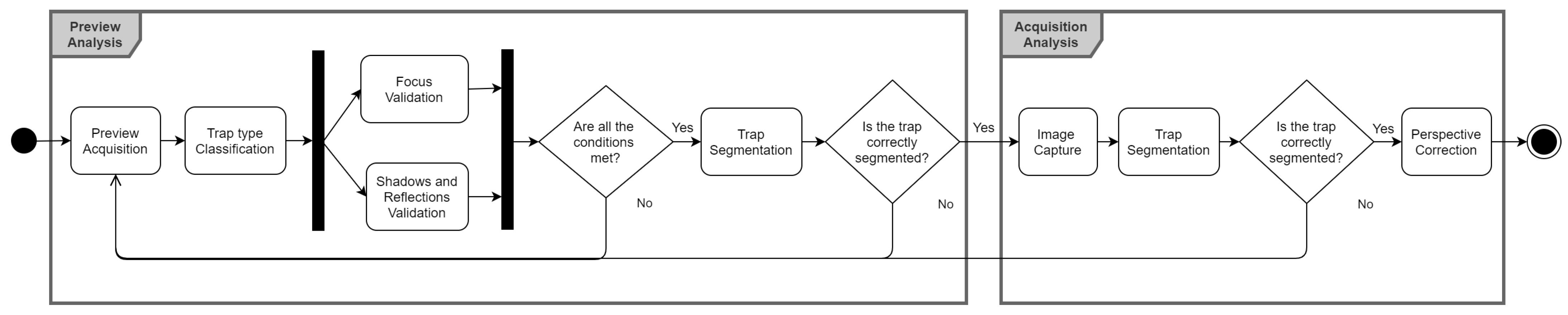
3. System Architecture

A mobile application module was designed in order to allow a hand-held acquisition of insect trap images and therefore the pest monitoring in vineyards. Requirements like the detailed control of image quality and adequacy were taken into account, in order to develop a solution that guides the user through the image acquisition process, by automatically assessing if requirements like image focus, absence of illumination artifacts, or the presence of the whole trap on the image are met.
The application relies on a set of computer vision algorithms that guides the user through the image acquisition process, and automatically acquires the image without the need of the user’s interaction when the quality and adequacy conditions of the image are automatically validated. The proposed methodology can be divided into two main steps: the Preview Analysis and the Acquisition Analysis, responsible for the processing of each camera preview frame and the acquired trap image, respectively (see Figure 1).
In order to automatically acquire a trap image, each preview frame must meet the requirements of four different modules: (i) focus validation; (ii) trap type classification; (iii) shadows and reflection validation; and (iv) trap segmentation. When a set of consecutive frames pass those conditions, an image is automatically acquired, a perspective correction step that relies on the corners of the detect trap segmentation mask being applied. It should be noted that the system is able to acquire images of both delta traps (DT) and chromotropic traps (CT), using almost the same processing flow, with just minor changes on individual steps that will be detailed in the following subsections.
The application validation flow is represented in Figure 1, and is processed sequentially. If any validation step fails, it will not continue to the next step and the process returns to the starting point. Despite being a procedure that is mostly processed sequentially, the focus and shadows/reflections’ validation steps are computed in parallel, in order to take advantage of the smartphones’ multi-thread capabilities and reduce the overall computational time.

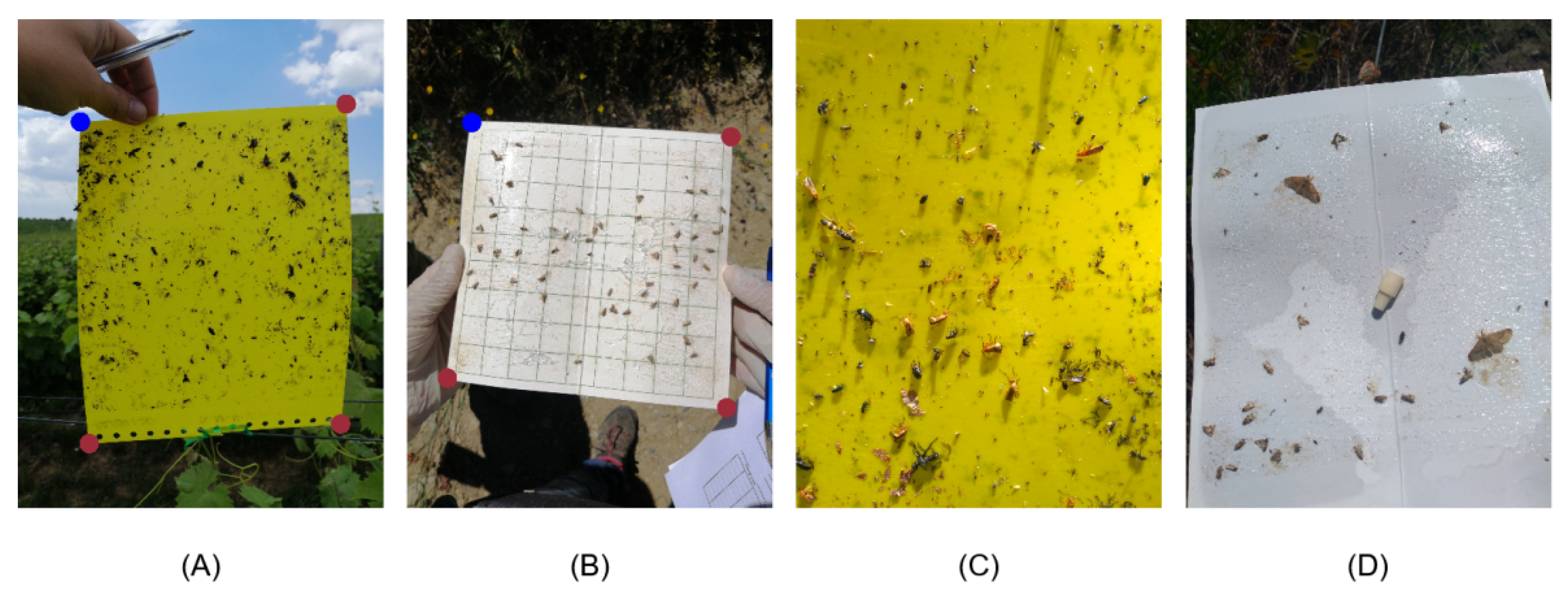
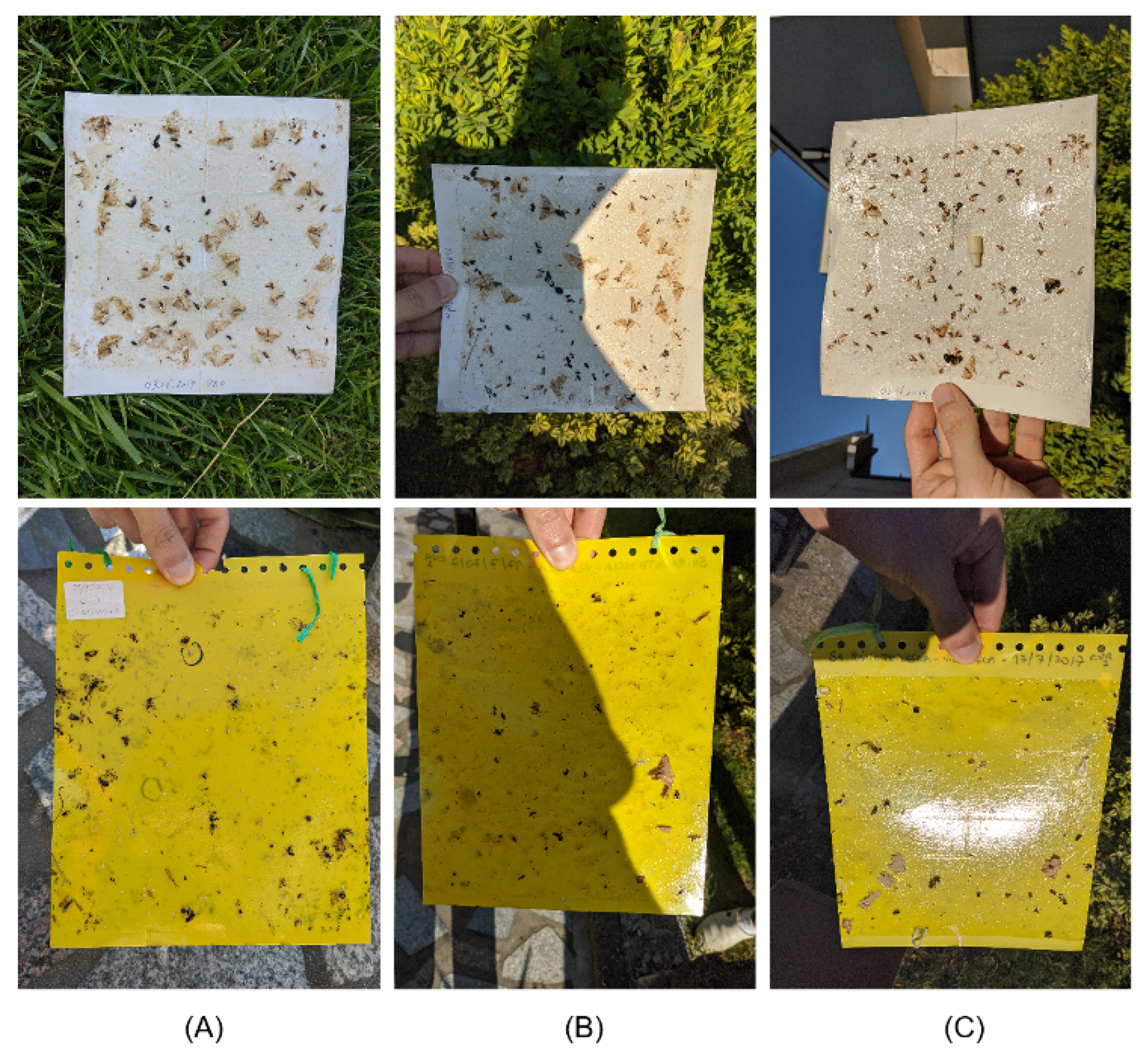
3.1. EyesOnTraps Dataset

In order to develop the automatic approaches for image quality and adequacy assessment, a dataset of 516 images was collected with trap images captured with different smartphones, in controlled and non-controlled environments, as well as simulating scenarios where the acquired images are out of focus, or with shadows and reflections present. In particular, the authors started by collecting a subset in a laboratory setting under well-controlled conditions (see Figure 2) using 28 traps previously collected on the field. This dataset was then complemented by a subset of trap images collected in a non-controlled environment, i.e., in three different vineyards by the target end-users of the system (winegrowers), during their weekly procedure to monitor the deployed traps (see Figure 3). It should be noted that both controlled and non-controlled subsets include DT and CT, with resolutions from 1224 × 1632 px to 2988 × 5312 px. The distribution of the images regarding the acquisition environment and trap type is shown in Table 1.
In order to support the development of the different system functionalities, three different subsets were created and manually labeled. The following sub-sections provides the details about these subsets, namely: (i) Image Focus Subset; (ii) Reflections and Shadows Subset; and (iii) Trap Segmentation Subset.

3.1.1. Image Focus Subset

The image focus subset aims to support the development of the automatic focus assessment step, and consists of a total of 205 images labelled as focused or unfocused (see Table 2). It was achieved by acquiring images of 20 DT and 18 CT, on which each CT results in two images, one for each side of the trap. Figure 2 shows images of DT focused, DT unfocused, CT focused, and CT unfocused, respectively, where the concern of acquiring images with the traps in different perspectives is also illustrated.

3.1.2. Reflections and Shadows Subset

The subset created to develop the the reflections and shadows assessment step consists of a total of 216 images manually labeled in three classes, as depicted in Table 3. In order to build this subset, some previously acquired images captured in an indoor setting were used, and additional images were acquired in a simulated non-controlled environment (outdoors with direct sun light), in order to produce a reasonable amount of images with significant reflections and shadows present.

3.1.3. Trap Segmentation Subset

The trap segmentation dataset includes a portion of the images used for previously described subsets and are representative of controlled and non-controlled environments. After an initial dataset analysis to assess the suitability of each image to be manually annotated in terms of trap location, some images had to be excluded. The exclusion criteria include images on which the borders or corners of the trap were not visible in the image, as well as repeated images of the same trap in similar conditions (perspective and illumination). After applying the referred exclusion criteria to the entire dataset of 516 images, 70 images do not have corners or borders of the trap, and 106 images of the same trap in similar perspectives and illumination conditions were discarded, resulting in the trap segmentation subset that includes a total of 340 images. For each image in the subset, a segmentation mask representing the trap location was manually annotated (see Figure 4).
It should be noted that all images contained in this subset have the four corners of the trap annotated, and will later be used as ground truth when assessing the performance of the proposed trap segmentation approach.

3.2. Image Focus Assessment Pipeline

Determining image focus is a crucial step to ensure that mobile-acquired trap images present the required quality to be further used for pest monitoring purposes. We developed a functional machine learning (ML) pipeline to assess image focus on CT and DT images, the respective development steps being described in the following sub-sections. As part of developing a suitable ML approach for real-life scenarios, we aimed to develop a model suitable for both high-end and low-end mobile devices. Thus, the selected ML model should be lightweight, for instance using the smallest combination of focus metrics while ensuring an acceptable performance, to operate smoothly under the most demanding computational constraints imposed by lower-end smartphones.

3.2.1. Feature Extraction

Prior to the feature extraction step, the images were cropped into a central square with a side equal to 50% of the smaller dimension (width or height) of the mobile-acquired trap image, depending on the image’s orientation. The resulting cropped square is then resized to 360 × 360 px. This pre-processing step aims to remove unnecessary information from the image (e.g., background) and make it more likely to only represent the trap, while the selected resized resolution is similar to the preview frame resolution that will be used on the mobile application. In order to compute the focus metrics that will be used as features by the ML model, the cropped image is converted to grayscale. Following previous works in the area of dermatology [23,24] and microscopy [25], where the use of artificially blurred images greatly enhanced the discriminative power of the focus metrics, in this work, we used a similar approach by applying a median blur filter with a kernel size of 5.
Regarding the feature extraction procedure, the set of focus metrics listed in Table 4 were independently computed for each grayscale and blurred image. It should be noted that many of these absolute focus metrics were previously proposed for focus assessment [26,27]. Additionally, we also followed more recent studies [23,24] by adding a new set of relative features that consists of the difference and the quotient between the obtained focus metrics for the grayscale and artificially blurred image. By merging all these absolute and relative focus metrics, a feature vector with a total of 788 features was obtained, with each metric properly being normalized through scaling (between 0 and 1).

3.2.2. Models Training and Optimization

The focus features detailed in the previous subsection were extracted for each image of the Image Focus Subset. The training, optimization, and selection of the best ML approach was performed using WEKA data mining software [28]. The model was trained using a 10-fold cross-validation strategy designed to optimize its accuracy. Experiments were performed with different classifiers: Linear SVM, Decision Trees, and Random Forests.

3.3. Shadows & Reflections Assessment Pipeline

An ML pipeline was developed to ensure that the acquired images did not present any illumination artifacts such as shadows or reflections, a key factor to ensure the quality and adequacy of the acquired trap images [16,17,18]. The main goal of this module is to avoid the use of trap images without suitable and homogeneous illumination, which might compromise not only posterior automated steps like trap segmentation or perspective correction, but also key tasks like the correct identification of insects for pest monitoring purposes.
In terms of feature extraction, the image is cropped into a central square with side equals to 50% of its smaller dimension (width or height) and resized to a 360 × 360 pixels resolution, as described in Section 3.2.1. Despite the considered metrics being mostly used for focus assessment purposes, many of them actually quantify image characteristics that are also relevant to detect shadows and reflections, such as the presence or relative changes in terms of texture and edges in the image [29,30]. Thus, we considered those same metrics, in order to explore if they also might be suitable for detecting the presence of uneven illumination conditions.
Regarding ML training and optimization, the same procedure detailed in Section 3.2.2 was applied. However, in this case, we have the particularity of having three different classes (as detailed in Section 3.1.2), also being observed through an exploratory analysis of the dataset collected that the presence of shadows and reflections on CT and DT may manifest quite distinctly in the images.
Due to the low number of DT images with reflections, and the specular reflections the different trap types present, an additional combination of experiments was considered, namely: (i) detect good and uneven illumination in both trap types using a single ML model, i.e., consider a 2-class problem by merging shadows and illumination labels in a single class; (ii) detect good and uneven illumination (2-class problem) in CT and DT separately, i.e., having two independent ML models for each trap type; (iii) detect good illumination, shadows and reflection (3-class problem) in both trap types using a single ML model; and (iv) detect good illumination, shadows and reflection (3-class problem) in both trap types separately through two independent ML models.

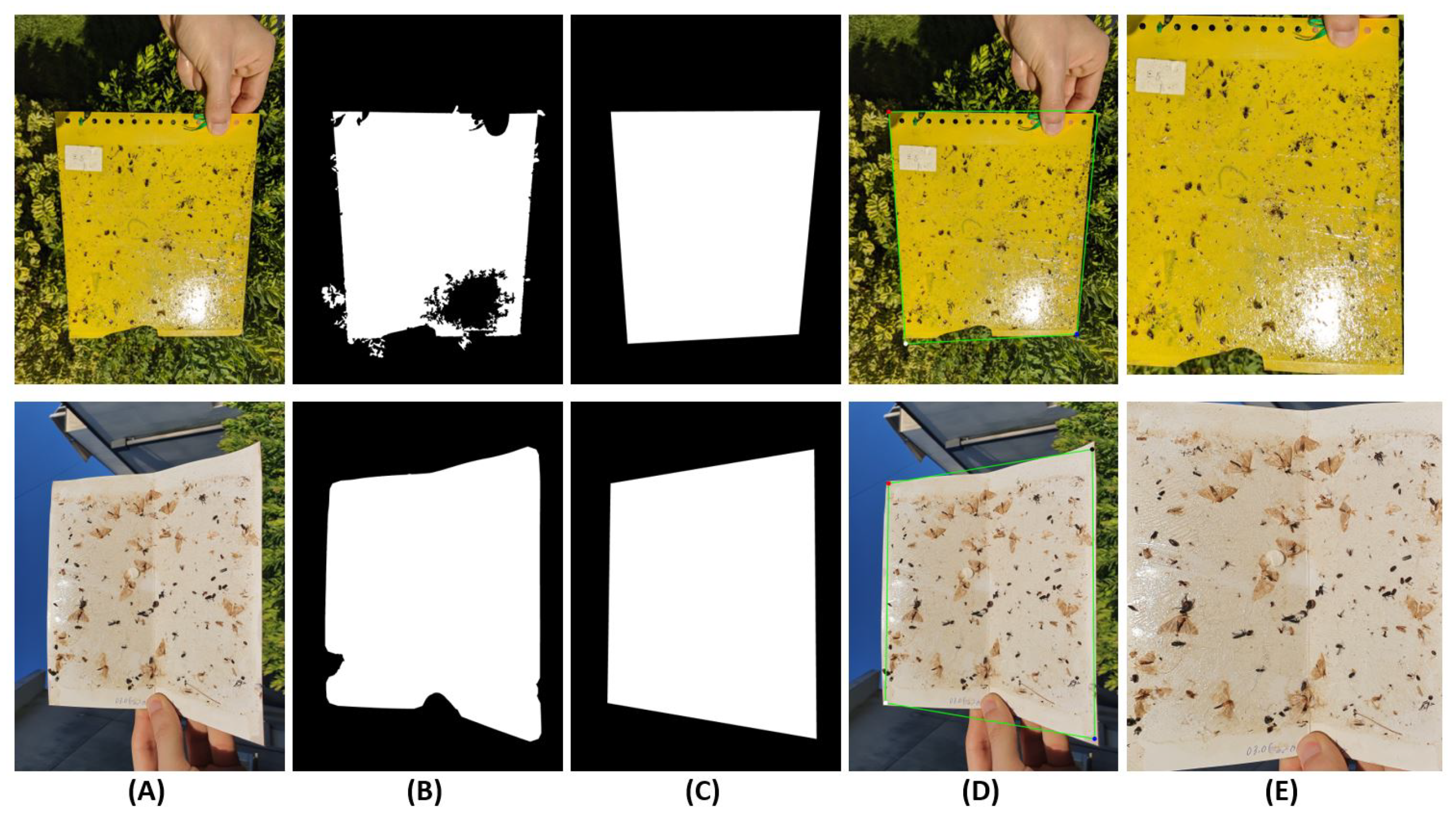
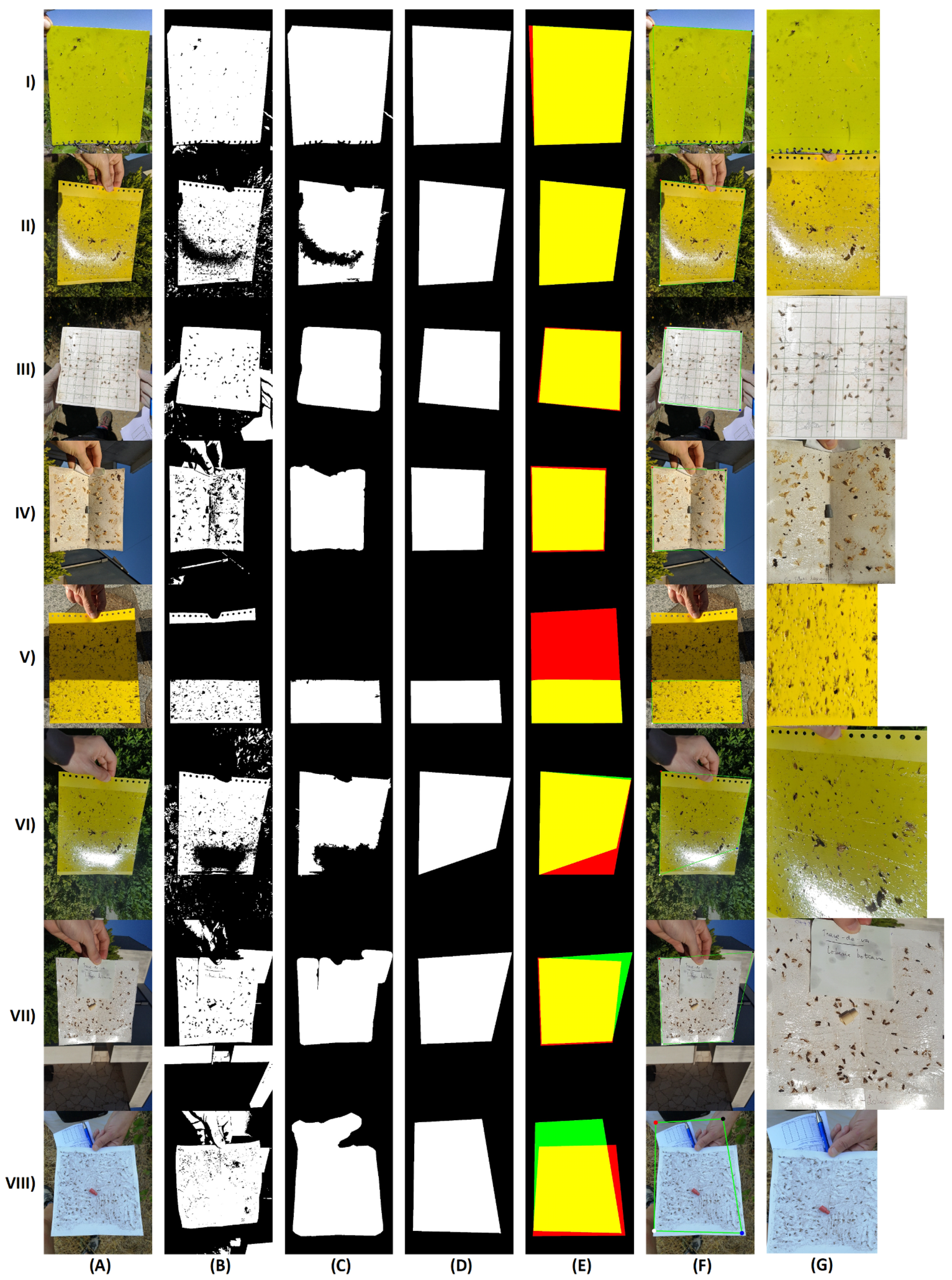
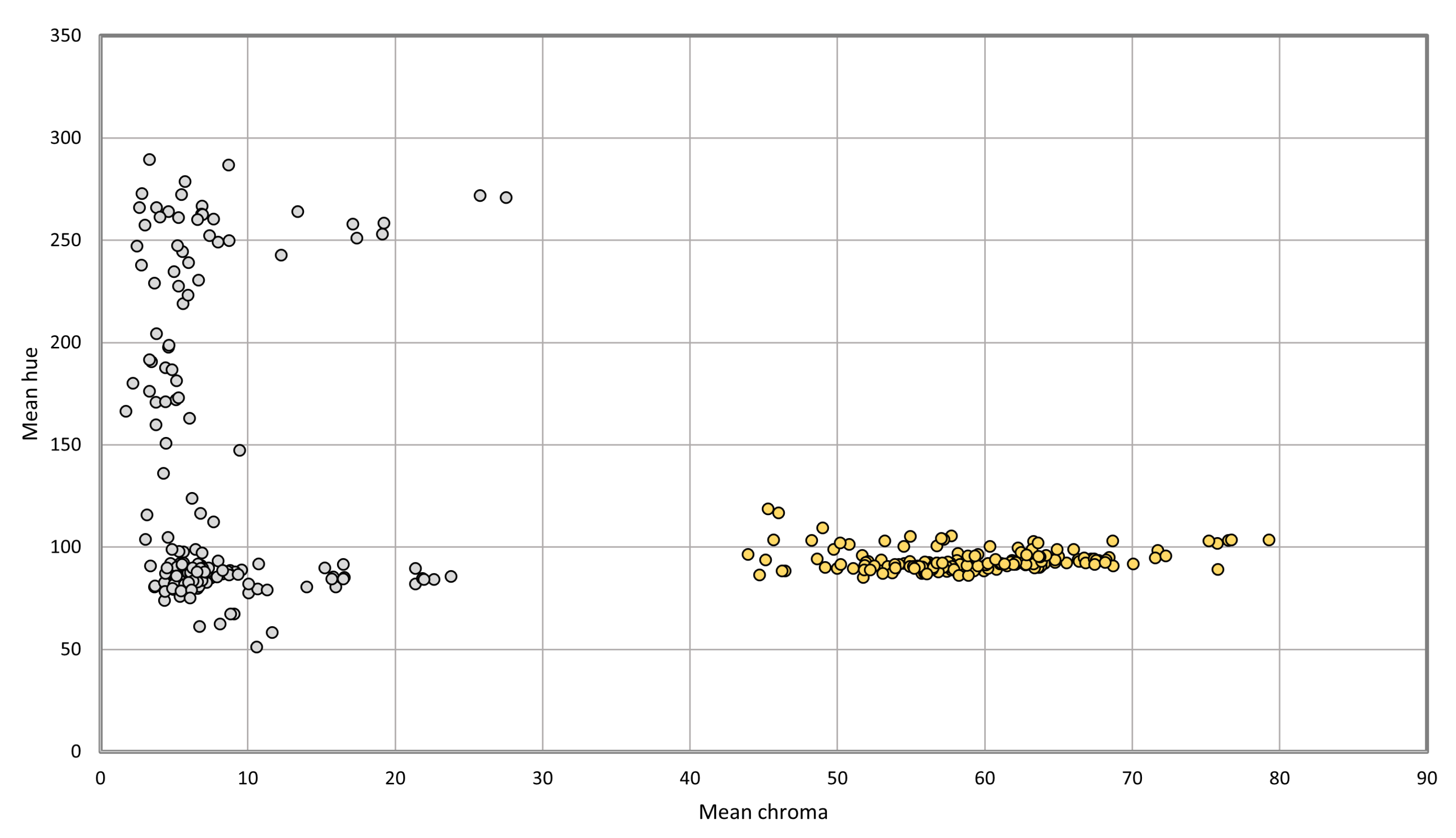
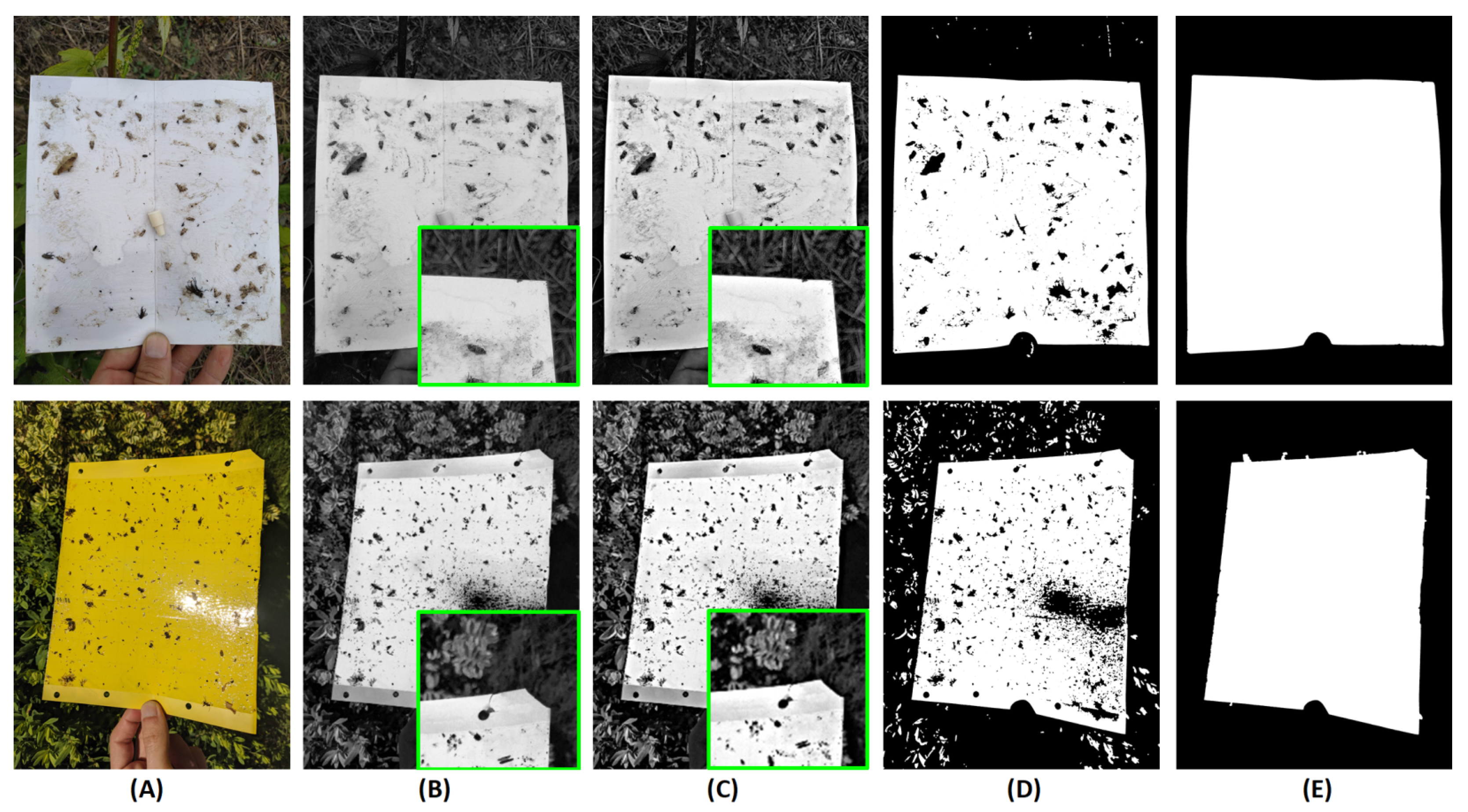
3.4. Trap Type Detection and Segmentation Pipeline

A robust trap segmentation is crucial to ensure that the trap is present and determine its specific location in the image. However, before determining the trap segmentation mask, the proposed approach starts by detecting the trap type on the image, i.e., classifying the image between DT and CT. The simplest and fastest approach found to achieve this was through the use of the L*C*h° (Lightness, Chroma, Hue) color space, due to its particular characteristics of being device independent and designed to match human perception. Thus, the image was converted from RGB to L*C*h° color space and an image crop procedure similar to the one detailed in Section 3.2.1 was applied, resulting in a squared image that only includes trap area. The mean value of Hue and Chroma channels were then extracted for each image, as shown in Figure 5. The data distribution already depicts a clear separation for DT and CT, which highlights the discriminative power of the used values to distinguish between trap type. Nevertheless, a decision tree was created using 10 fold-cross validation, in order to find the optimal threshold.
Depending on the trap type detected, a grayscaled image is generated from the acquired image. This pre-processing step differs based on the trap type, in order to increase the contrast between the trap and the background. In particular, for DT, this is achieved by considering the minimum RGB intensity for each pixel, while, for CT, the trap contrast is increased by subtracting the G channel from the B channel. For both cases, a normalization was applied (see Figure 6B).
To further facilitate the segmentation task, the trap sharpness was also increased via unsharp masking, a procedure that subtracts a smoothed version of the original image in a weighted way, so the intensity values of constant areas remain constant (see Figure 6C).
Particularly, the smoothed image was obtained by blurring the original grayscale image I G r a y using a Gaussian filter with a fixed window radius of 50, a blurred image I B l u r being obtained which is then combined with the I G r a y , according to the weights detailed in Equation (1):
I S h a r p = 1.5 × I G r a y 0.5 × I B l u r
Finally, the algorithm used for trap segmentation was based on Otsu’s Method [31], a well-known histogram shape-based image thresholding routine, very computationally efficient, and thus suitable to run in real time on mobile devices (see Figure 6D). This method assumes that the input image has two classes of pixels and calculates the threshold that minimizes the intra-class variance. In order to smooth the trap border by connecting unconnected blobs on the limits of the trap, a closing morphological operation with an elliptical structuring element of size 9 is applied. The segmentation task terminates with an area filtering step, being only selected the biggest blob as the representative for the trap segmentation mask, and the remaining inner structures inside this mask were removed using a flood fill algorithm (see Figure 6E).

3.5. Trap Perspective Correction Pipeline

Both DT and CT have usually square or rectangular shapes, but, when viewed from different perspectives, they can assume distinct quadrilateral shapes in the image (e.g., trapeziums). In order to standardize the image capture of traps and turn it independent of the perspective selected by the user during the image acquisition process, a perspective correction methodology was used to ensure that the trap in the corrected image will always have a square or rectangular shape. This approach receives as input the segmentation mask previously obtained (see Figure 7B), and, in order to find the four corners of the trap, a polygonal approximation method was applied based on the Douglas–Peucker algorithm [32]. The method recursively approximates the polygon obtained from the convex hull of the trap contours to another polygon with just four vertices, so that the distance between them is less or equal to the specified precision (see Figure 7C). The resulting corners are sorted (see Figure 7D), and used to compute the 3 × 3 perspective transform matrix [33], leading to the desired perspective transformation (see Figure 7E).
Due to the variable dimensions of traps, an additional step is required to ensure the image presents the correct aspect ratio. In order to achieve this, we used a previously proposed technique [34] which assumes that the rectangular trap is projected in a plane perpendicular to the camera’s pinhole. By relating the two concurrent vectors of the plane, we are able to compute the correct aspect ratio of the trap, and consequently apply an image resize step to ensure it (see Figure 7E).

4. Results and Discussion

4.1. Image Focus Assessment Results

Following the methodology described in Section 3.2.2, the weighted classification results for the different ML classifiers, in terms of different performance metrics, are presented in Table 5.
The real-time execution in mobile devices being one major requirement, the trade-off between performance and computational complexity was crucial to select the most suitable model. The Decision Tree model highlighted in Table 5, which achieves a result close to the best classification model, while being the lightest model, since it uses a single focus metric (mean Thresholded Absolute Gradient of the quotient between the blurred and original image), was included in the pipeline.

4.2. Shadows & Reflections Assessment Results

The following tables present the results for the validation of the present of illumination artifacts as detailed in Section 3.3. As previously detailed, we designed a series of experimental combinations to select the most suitable approach, namely: (i) if the ML model should tackle a two-class problem (good and uneven illumination, by merging shadows and illumination labels in a single class) or a 3-class problem (good illumination, shadows and reflection); and (ii) if we should consider a single ML model (i.e., suitable for both trap types) or two independent ML models for each trap type. Table 6 shows the weighted classification results for the single ML model approach, considering both 2-class and 3-class scenarios.
Regarding the experiments with independent ML models for each trap type (considering both 2-class and 3-class scenarios), Table 7 shows the weighted classification results for the independent ML model approach just for CT, while Table 8 shows the weighted classification results for the independent ML model approach just for DT. Considering the trade-off between performance and complexity of the different models, we considered that the best option for our solution would be to use independent ML models for each trap type (highlighted in Table 7 and Table 8). Each of these models will tackle a 2-class classification problem, based on a Decision Tree that remarkably only needs a small number of features to achieve interesting results. In particular, the mean value of Variance for the blurred image is the feature selected for the CT model, while the DT model uses the the difference between the skew values of the Normalized Variance of the original and the blurred image; and the minimum value of normalized variance of the blurred image.

4.3. Trap Type Detection & Segmentation Results

In terms of the proposed approach to detect the trap type present on the image, we achieved a 100% accuracy score using the mean Chroma value channel from the L*C*h° color space. Given the data distribution depicted in Figure 5, this perfect performance was already expected. In particular, an optimal threshold of 37.53 for mean Chroma value was obtained, which was achieved through the train of a Decision Tree model using 10 fold-cross validation.
Regarding the evaluation of the proposed methodology for trap segmentation, we used as a performance metric the Jaccard index (JA) between the obtained segmentation mask (after polygonal approximation) and the respective ground truth annotation. These results are shown in Table 9, where we can see that an overall JA of 96.7% was achieved, a performance that fits the requirements needed to include this approach in our solution. Nevertheless, we noticed that the segmentation performance significantly varies with the conditions in which the images were acquired. Thus, in Table 9, we also detail the segmentation performance for the following subsets: (i) CT image acquired in controlled environment (CT-CtE); (ii) CT image acquired in non-controlled environment (CT-NCtE); (iii) DT image acquired in controlled environment (DT-CtE); and (iv) DT image acquired in a non-controlled environment (DT-NCtE).
Figure 8 presents some examples of segmentation results with high (I–IV) and low (V–VIII) mean JA. It is clear that the proposed approach is capable of properly handling artifacts like reflections (see Figure 8(II)) and structures overlapped to the trap with similar color (see Figure 8(III–IV)). However, the presence of extreme shadows and reflections might greatly compromise the segmentation performance (see Figure 8(V–VI)), as well as overlapped structures with almost identical colors (see Figure 8(VII–VIII)).

4.4. Trap Perspective Correction Results

Regarding the analysis of the the perspective correction results, it should be noted that the performance of this approach is directly related with the successful segmentation of the trap, i.e., the perspective will only be successfully corrected when a good segmentation is achieved through the 4-point polygonal approximation. This is clearly seen in Figure 8: the images I to IV, which present a suitable perspective transformation, have a JA between 0.976 and 0.935, while the images V to VIII, which present an unsuitable perspective transformation, have a JA index value ranging from 0.383 to 0.872. Considering that the mean JA for the entire dataset is 0.967, we can then assume that a perspective transformation was successfully achieved in the vast majority of the dataset, a fact that was confirmed by the authors through the visual analysis of the perspective transform output for each image.
In order to illustrate the suitability of the perspective transform procedure when a good trap segmentation is achieved, in Figure 9, we show three photos acquired with abrupt perspective changes for the same trap. As we can see in the perspective transform result, regardless of the perspective in which the images were acquired, the corrected image is always remarkably similar, which highlights the potential of this approach to standardize the image acquisition process of insect traps. However, it should be noted that images which need demarked perspective corrections (e.g., bottom CT image (A) in Figure 9 will be impacted in terms of image quality, regardless of the successful transformation to the rectangular shape. Image pixelization on the corrected image might be one of the side effects, since the objects in the demarked perspective have less pixels to represent them.

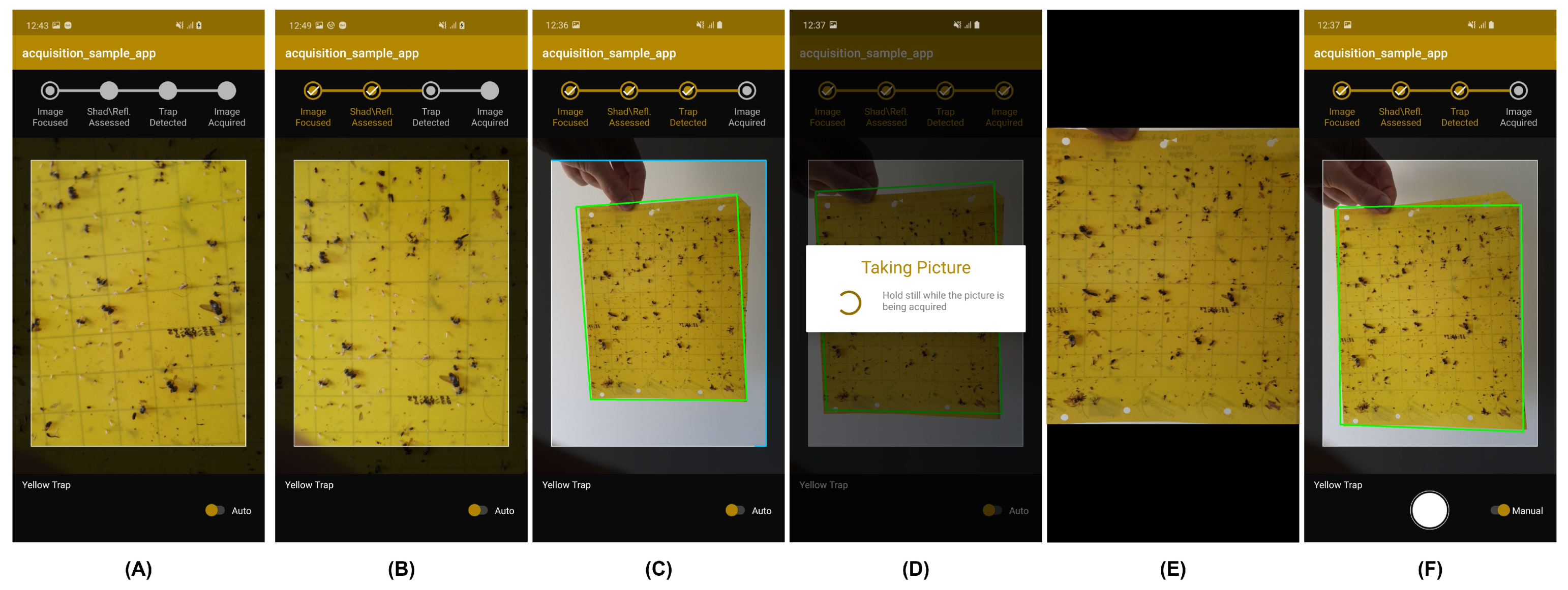
4.5. Mobile Application

Based on the results reported in previous sections, the proposed pipeline was deployed as an Android application, in order to ensure that the mobile-acquired trap images present the required level of adequacy and quality. In particular, the developed application integrated all the previously referred modules in the sequence depicted in Figure 1, providing real-time feedback to the user during preview analysis in terms of: (i) focus assessment; (ii) shadow and reflections assessment; (iii) trap type detection; and (iv) trap segmentation. When a set of consecutive frames passes those conditions (in order to ensure stability), an image is automatically acquired (see Figure 10A–D), the perspective correction procedure being further applied (see Figure 10E).
In addition, if the system is not able to acquire the image automatically, the user may perform the acquisition using the manual mode of the application. However, in the manual acquisition mode, the results of the methods previously described can still be visualized, and the user is responsible to press the camera button for triggering the capture of an image (see Figure 10F).
In order to access the feasibility to execute the propose pipeline in devices with different computational capabilities, acquisitions were performed using a high-end smartphone (Samsung S10) and a low-end smartphone (Samsung S6). The mean and standard deviation times for the preview analysis and the perspective correction procedure applied to the acquired image measured for both devices are detailed in Table 10. The reported values were computed based on 10 runs of each process, for each device and acquiring images of both trap types.
By analyzing these results, it is clear that the processing times for the Preview Analysis are significantly slower for the low-end device. However, the reported processing times can still be considered suitable for the purpose of the designed application. Regarding the perspective correction procedure, which also includes the trap’s segmentation of the acquired image, the demarcated increase in processing time when compared with the Preview Analysis can be explained by the higher resolution of the acquired image used in this step, when compared with the preview image used in the Preview Analysis. Nevertheless, and despite the considerable amount of time required, we consider this process also suitable for both high-end and low-end devices, since it can be performed in a background task, resulting in a lower impact on the usability of the application.

5. Conclusions and Future Work

The work presented here combines the use of a custom AI image acquisition system with Android mobile devices to create further insect pest monitoring technology options for field applications. Our image acquisition system validates the quality and adequacy of the mobile-acquired trap images in real-time, by automatically assessing the focus and illumination of the image, while ensuring that an insect trap is present via a trap type detection procedure coupled to a segmentation step. In order to train and validate these different validation steps, a dataset with a total of 516 images including images of both DT and CT was collected. The dataset was divided into three subsets, such as the image focus subset, the reflections and shadows subset, and the trap segmentation subset, to support the development and validation of the different considered functionalities, being manually annotated for each particular purpose.
The proposed approaches achieved an accuracy of 84% regarding focus assessment, an accuracy of 96% and 80% regarding the shadows and/or reflections on CT and DT traps, respectively, and a Jaccard index value of 97% for the segmentation approach. Furthermore, the proposed pipeline was embedded in an Android application, in order to ensure that the mobile-acquire trap images present the required level of adequacy and quality.
In terms of future work, we plan to perform further tests to validate the solution in a real life scenario, as well as assessing the impact that the perspective correction approach has on an image’s quality, when applied to abrupt trap perspectives. Additionally, we aim to explore effective ways to segment traps with higher levels of deformation (e.g., the existence of bends or folds), without compromising the results attained in the more frequent and simpler scenarios. In order to address this issue, besides the additional adjustments that would be required on the segmentation and following perspective correction steps, the ground truth annotation masks will probably need to be re-annotated with a higher detail and granularity (e.g., increase the number of annotation points in the trap border). The performance of the segmentation process and the trap’s perspective correction should also be further studied in future work, mainly on low-end devices when applied to DT.
As a final note, this work represents only a component of a mobile-based solution for pest prevention in vineyards that is currently being developed. Thus, we aim to integrate this methodology into a decision support tool for winegrowers and taxonomy specialists that allows for: (i) ensuring the adequacy and quality of mobile-acquired images of DT and CT; (i) providing an automated detection and counting of key vector insects, like Lobesia botrana (european grapevine moth), Empoasca vitis (smaller green leafhopper) or Scaphoideus titanus (American grapevine leafhopper); and (iii) improving and anticipating treatment recommendations for the detected pests.

Author Contributions

Conceptualization, L.R. and P.F.; methodology, L.R. and P.F.; software, L.R. and P.F.; validation, L.R. and P.F.; formal analysis, L.R. and P.F.; investigation, P.F. and L.R.; resources, T.N., A.F. and C.C.; data curation, P.F.; writing—original draft preparation, P.F.; writing—review and editing, A.F., C.C., L.R., P.F. and T.N.; visualization, P.F.; supervision, L.R.; project administration, L.R.; funding acquisition, L.R., T.N. and C.C. All authors have read and agreed to the published version of the manuscript.

Funding

This research was funded by European Regional Development Fund (ERDF) in the frame of Norte 2020 (Programa Operacional Regional do Norte), through the project EyesOnTraps+—Smart Learning Trap and Vineyard Health Monitoring, NORTE-01-0247-FEDER-039912.

Institutional Review Board Statement

Not applicable.

Informed Consent Statement

Not applicable.

Data Availability Statement

Not applicable.

Acknowledgments

The authors would like to give a special thanks to the stakeholders of the wine sector that collaborated on the data collection phase, namely Sogevinus Quintas SA, Adriano Ramos Pinto—Vinhos SA and Sogrape Vinhos, SA; and to Direcção Regional de Agricultura e Pescas do Norte (DRAPN) for providing chromotropic traps.

Conflicts of Interest

The authors declare no conflict of interest.

Abbreviations

The following abbreviations are used in this manuscript:
AIArtificial Intelligence
MLMachine Learning
CTChromotropic Traps
DTDelta Traps
CtEControlled Environment
NCtENon-Controlled Environment

References

  1. International Organisation of Vine and Wine (OIV). State of the World Vitivinicultural Sector in 2019; International Organisation of Vine and Wine: Paris, France, 2020. [Google Scholar]
  2. International Organisation of Vine and Wine (OIV). 2019 Statistical Report on World Vitiviniculture; International Organisation of Vine and Wine: Paris, France, 2019. [Google Scholar]
  3. Plants Vital to Human Diets but Face Growing Risks From Pests and Diseases. 2016. Available online: http://www.fao.org/news/story/en/item/409158/icode/ (accessed on 22 March 2021).
  4. Monitoring Whitefly and Thrips—Sticky Traps Plus Scouting Delivers Best Results. Available online: https://www.biobestgroup.com/en/news/monitoring-whitefly-and-thrips-sticky-traps-plus-scouting-delivers-best-results (accessed on 24 November 2020).
  5. Yao, Q.; Xian, D.-X.; Liu, Q.-J.; Yang, B.-J.; Diao, G.-Q.; Tang, J. Automated Counting of Rice Planthoppers in Paddy Fields Based on Image Processing. J. Integr. Agric. 2014, 13, 1736–1745. [Google Scholar] [CrossRef]
  6. Ünlü, L.; Akdemir, B.; Ögür, E.; Şahin, I. Remote Monitoring of European Grapevine Moth, Lobesia botrana (Lepidoptera: Tortricidae) Population Using Camera-Based Pheromone Traps in Vineyards. Turk. J. Agric. Food Sci. Technol. 2019, 7, 652. [Google Scholar] [CrossRef] [Green Version]
  7. García, J.; Pope, C.; Altimiras, F. A Distributed K-Means Segmentation Algorithm Applied to Lobesia botrana Recognition. Complexity 2017, 2017, 5137317. [Google Scholar] [CrossRef] [Green Version]
  8. DTN. DTN Smart Trap for Producer. 2020. Available online: https://www.dtn.com/agriculture/producer/dtn-smart-trap/ (accessed on 24 November 2020).
  9. TRAPVIEW. 2020. Available online: https://www.trapview.com/en/ (accessed on 24 November 2020).
  10. Semios. Precision Agriculture Technology that Helps Growers Worry Less. 2020. Available online: https://semios.com/ (accessed on 24 November 2020).
  11. FARMSENSE. 2020. Available online: https://www.farmsense.io/ (accessed on 24 November 2020).
  12. TARVOS. 2020. Available online: https://tarvos.ag/ (accessed on 24 November 2020).
  13. Scoutbox. 2020. Available online: https://www.agrocares.com/en/products/scoutbox/ (accessed on 24 November 2020).
  14. Fang, Y.; Zhu, H.; Zeng, Y.; Ma, K.; Wang, Z. Perceptual Quality Assessment of Smartphone Photography. In Proceedings of the IEEE/CVF Conference on Computer Vision and Pattern Recognition (CVPR), Seattle, WA, USA, 13–19 June 2020. [Google Scholar]
  15. Robisson, P.; Jourdain, J.B.; Hauser, W.; Viard, C.; Guichard, F. Autofocus measurement for imaging devices. Electron. Imaging 2017, 2017, 209–218. [Google Scholar] [CrossRef] [Green Version]
  16. Tiwari, A.; Singh, P.; Amin, S. A survey on Shadow Detection and Removal in images and video sequences. In Proceedings of the 2016 6th International Conference—Cloud System and Big Data Engineering, Noida, India, 14–15 January 2016; pp. 518–523. [Google Scholar] [CrossRef]
  17. Morgand, A.; Tamaazousti, M. Generic and real-time detection of specular reflections in images. In Proceedings of the 2014 International Conference on Computer Vision Theory and Applications (VISAPP), Lisbon, Portugal, 5–8 January 2014; pp. 274–282. [Google Scholar]
  18. Jiddi, S.; Robert, P.; Marchand, E. Detecting Specular Reflections and Cast Shadows to Estimate Reflectance and Illumination of Dynamic Indoor Scenes. IEEE Trans. Vis. Comput. Graph. 2020. [Google Scholar] [CrossRef] [PubMed] [Green Version]
  19. Al-amri, S.S.; Kalyankar, N.V.; Khamitkar, S.D. Image segmentation by using edge detection. Int. J. Comput. Sci. Eng. 2010, 2, 804–807. [Google Scholar]
  20. Mukherjee, S.; Mukherjee, D. Segmentation of Circular and Rectangular Shapes in an Image Using Helmholtz Principle. In Proceedings of the 2008 Sixth Indian Conference on Computer Vision, Graphics & Image Processing, Bhubaneswar, India, 16–19 December 2008; pp. 657–664. [Google Scholar] [CrossRef]
  21. Guerzhoy, M.; Zhou, H. Segmentation of Rectangular Objects Lying on an Unknown Background in a Small Preview Scan Image. In Proceedings of the 2008 Canadian Conference on Computer and Robot Vision, Windsor, ON, Canada, 28–30 May 2008; pp. 369–375. [Google Scholar] [CrossRef]
  22. Moreira, D.; Alves, P.; Veiga, F.; Rosado, L.; Vasconcelos, M.J.M. Automated Mobile Image Acquisition of Macroscopic Dermatological Lesions. In Proceedings of the 14th International Joint Conference on Biomedical Engineering Systems and Technologies, Online Streaming, 11–13 February 2021. [Google Scholar]
  23. Faria, J.; Almeida, J.; Vasconcelos, M.J.M.; Rosado, L. Automated Mobile Image Acquisition of Skin Wounds Using Real-Time Deep Neural Networks. In Medical Image Understanding and Analysis: Proceedings of the 23rd Conference, MIUA 2019, Liverpool, UK, 24–26 July 2019; Zheng, Y., Williams, B.M., Chen, K., Eds.; Springer International Publishing: Cham, Switzerland, 2020; pp. 61–73. [Google Scholar]
  24. Alves, J.; Moreira, D.; Alves, P.; Rosado, L.; Vasconcelos, M.J.M. Automatic focus assessment on dermoscopic images acquired with smartphones. Sensors 2019, 19, 4957. [Google Scholar] [CrossRef] [PubMed] [Green Version]
  25. Rosado, L.; Silva, P.T.; Faria, J.; Oliveira, J.; Vasconcelos, M.J.M.; da Costa, J.M.C.; Elias, D.; Cardoso, J.S. μSmartScope: Towards a Fully Automated 3D-printed Smartphone Microscope with Motorized Stage. In Biomedical Engineering Systems and Technologies: 10th International Joint Conference, BIOSTEC 2017, Porto, Portugal, 21–23 February 2017; Communications in Computer and Information Science Book Series; Springer: Cham, Switzerland, 2018; Volume 881. [Google Scholar]
  26. Pertuz, S.; Puig, D.; García, M. Analysis of focus measure operators in shape-from-focus. Pattern Recognit. 2013, 46, 1415–1432. [Google Scholar] [CrossRef]
  27. Santos, A.; Ortiz-de Solorzano, C.; Vaquero, J.J.; Peña, J.; Malpica, N.; Del Pozo, F. Evaluation of autofocus functions in molecular cytogenetic analysis. J. Microsc. 1998, 188, 264–272. [Google Scholar] [CrossRef] [PubMed] [Green Version]
  28. Frank, E.; Hall, M.A.; Holmes, G.; Kirkby, R.; Pfahringer, B.; Witten, I.H. Weka: A machine learning workbench for data mining. In Data Mining and Knowledge Discovery Handbook: A Complete Guide for Practitioners and Researchers; Maimon, O., Rokach, L., Eds.; Springer: Berlin, Germany, 2005; pp. 1305–1314. [Google Scholar]
  29. Wang, S.; Zheng, H. Clustering-based shadow edge detection in a single color image. In Proceedings of the 2013 International Conference on Mechatronic Sciences, Electric Engineering and Computer (MEC), Shenyang, China, 20–22 December 2013; pp. 1038–1041. [Google Scholar] [CrossRef]
  30. Xu, L.; Qi, F.; Jiang, R. Shadow Removal from a Single Image. In Proceedings of the Sixth International Conference on Intelligent Systems Design and Applications, Jian, China, 16–18 October 2006; pp. 1049–1054. [Google Scholar] [CrossRef]
  31. Otsu, N. A Threshold Selection Method from Gray-Level Histograms. IEEE Trans. Syst. Man Cybern. 1979, 9, 62–66. [Google Scholar] [CrossRef] [Green Version]
  32. Douglas, D.; Peucker, T. Algorithms for the reduction of the number of points required to represent a digitized line or its caricature. Cartogr. Int. J. Geogr. Inf. Geovis. 1973, 10, 112–122. [Google Scholar] [CrossRef] [Green Version]
  33. Szeliski, R. Computer Vision: Algorithms and Applications, 1st ed.; Springer: Berlin/Heidelberg, Germany, 2010. [Google Scholar]
  34. Zhang, Z.; He, L.-W. Whiteboard scanning and image enhancement. Digit. Signal Process. 2007, 17, 414–432. [Google Scholar] [CrossRef]
Figure 1. Application flow for image quality and adequacy validation.
Agronomy 11 00731 g001
Figure 2. Illustrative images labeled as: (A) focused; and (B) unfocused.
Agronomy 11 00731 g002
Figure 3. Illustrative images labeled as: (A) good illumination; (B) with shadows; (C) with reflections.
Agronomy 11 00731 g003
Figure 4. Illustrative images of: CT (A) and DT (B) images with respective ground truth trap location; (C) excluded image (trap border not visible); and (D) excluded image (not all trap corners appear within the field of view).
Agronomy 11 00731 g004
Figure 5. Data distribution of mean Hue and Chroma values for DT (grey) and CT (yellow).
Agronomy 11 00731 g005
Figure 6. Trap segmentation: (A) original RGB image; (B) grayscale image; (C) sharpening; (D) Otsu’s segmentation; (E) post-processing (morphological operations, area filtering, and hole-filling).
Agronomy 11 00731 g006
Figure 7. Perspective correction methodology: (A) original image; (B) trap segmentation mask; (C) segmentation mask from polygonal approximation; (D) corner points from polygonal approximation; (E) transformed image with corrected perspective.
Agronomy 11 00731 g007
Figure 8. Illustrative images of high JA (I to IV) and low JA (V to VIII) for trap segmentation results: (A) original image; (B) Otsu’s segmentation; (C) post-processing (morphological operations, area filtering and hole-filling); (D) segmentation with polygonal approximation; (E) comparison image between segmentation and ground truth; (F) corner points from polygonal approximation; (G). Transformed image with corrected perspective. (In comparison images: yellow—true positives; red—false negatives; green—false positives; black—true negatives.)
Agronomy 11 00731 g008
Figure 9. Examples of perspective correction results: CT (A) and DT (C) images from the same trap, with overlapped corners from the polygonal approximation process; Respective perspective correction results for CT (B) and DT (D) images.
Agronomy 11 00731 g009
Figure 10. Android application screenshots: (A) unfocused image; (B) focused and good illumination; (C) trap detected; (D) automatic image capture; (E) perspective correction; and (F) manual mode.
Agronomy 11 00731 g010
Table 1. Dataset image distribution regarding acquisition environment and trap type.
Trap Type#Images Controlled Environment#Images Non-Controlled EnvironmentTotal
DT14190231
CT25332285
All394122516
Table 2. Dataset image distribution regarding labelled data for the image focus assessment step.
Trap Type#Images Focused#Images UnfocusedTotal
DT332760
CT7669145
All102103205
Table 3. Dataset image distribution regarding labelled data for the reflections and shadows validation step.
Trap Type#Control Images#Images with Reflections#Images with ShadowsTotal
DT5152278
CT533748138
All1044270216
Table 4. Summary of the features extracted for focus assessment.
GroupFeature NameExtracted Metrics
GradientGaussian Derivativemax, std, min, max, sum, L2norm, skew, kurt
Squared Gradientmax, std, min, max, sum, L2norm, skew, kurt
Thresholded Abs. Grad.max, std, min, max, sum, L2norm, skew, kurt
Gradient Energymax, std, min, max, sum, L2norm, skew, kurt
Tenengradmax, std, min, max, sum, L2norm, skew, kurt
Tenengrad Variancemax, std, min, max, sum, L2norm, skew, kurt
StatisticGray Level Variancemax, std, min, max, sum, L2norm, skew, kurt
Norm. Gray L. Variancemax, std, min, max, sum, L2norm, skew, kurt
Histogram RangeRange (grey, blue, green, red)
Histogram EntropyEntropy (blue, green, red)
LaplacianModified Laplacianmax, std, min, max, sum, L2norm, skew, kurt
Energy of Laplacianmax, std, min, max, sum, L2norm, skew, kurt
Diagonal of Laplacianmax, std, min, max, sum, L2norm, skew, kurt
Variance of Laplacianmax, std, min, max, sum, L2norm, skew, kurt
Laplacian Filtermax, std, min, max, sum, L2norm, skew, kurt
DCTDCT Energy Ratiomax, std, min, max, sum, L2norm, skew, kurt
DCT Reduced Energy Ratiomax, std, min, max, sum, L2norm, skew, kurt
Modified DCTmax, std, min, max, sum, L2norm, skew, kurt
OtherBrenner’s Measuremax, std, min, max, sum, L2norm, skew, kurt
Image Curvaturemax, std, min, max, sum, L2norm, skew, kurt
Image Contrastmax, std, min, max, sum, L2norm, skew, kurt
Spatial Frequencymax, std, min, max, sum, L2norm, skew, kurt
Vollath’s Autocorrelationmax, std, min, max, sum, L1norm, L2norm, skew, kurt
Vollath’s Standard Deviationmax, std, min, max, sum, L1norm, L2norm, skew, kurt
Helmli and Scheres Mean Methodmax, std, min, max, sum, L2norm, skew, kurt
Marziliano MetricsumX, meanX, sumY, meanY
Table 5. Classification results image focus assessment.
ModelAccuracyRecallPrecisionF1#Features
Linear SVM0.8840.8840.8870.882788
Random Forest0.8950.8950.8990.894495
Decision Tree0.8550.8550.8550.8534
Decision Tree0.8430.8430.8430.8431
Table 6. Classification results for shadows and reflections using a single ML model for DT and CT.
#ClassesModelAccuracyRecallPrecisionF1#Features
3-class problemDecision Tree0.8570.8570.8680.8572
3-class problemRandom Forest0.9290.9290.9280.928185
2-class problemRandom Forest0.8940.8940.8940.894587
2-class problemDecision Tree0.8220.8220.8230.8221
Table 7. Classification results for shadows and reflections using an independent ML model for CT.
Train ConditionsModelAccuracyRecallPrecisionF1#Features
3-class problemRandom Forest0.9460.9460.9510.946403
3-class problemDecision Tree0.9570.9570.9570.9573
2-class problemDecision Tree0.9620.9620.9630.9621
Table 8. Classification results for shadows and reflections using an independent ML model for DT.
Train ConditionsModelAccuracyRecallPrecisionF1#Features
3-class problemRandom Forest0.8460.8460.8040.823210
3-class problemDecision Tree0.7950.7950.7950.7702
2-class problemRandom Forest0.8330.8330.8450.832237
2-class problemDecision Tree0.7960.7960.7930.7962
Table 9. Trap segmentation performance results: Mean and STD Jaccard index values between the obtained segmentation mask (after polygonal approximation) and the respective ground truth annotation. CtE—controlled environment, NCtE—non-controlled environment, CT—chromotropic trap; DT—delta trap.
Entire DatasetCT-CtE SubsetCT-NCtE SubsetDT-CtE SubsetDT-NCtE Subset
JA Mean0.9670.9890.9360.9900.936
JA STD0.0760.0290.1080.0120.109
Table 10. Processing times for high-end and low-end mobile devices.
CTDT
High-EndLow-EndHigh-EndLow-End
Preview Analysis Time (ms)mean55615088021784
std36183135195
Perspective Correction Time (ms)mean509114,92221,40944,581
std592157412,0557665
Publisher’s Note: MDPI stays neutral with regard to jurisdictional claims in published maps and institutional affiliations.

