Article

Machine-Learning Approach Using SAR Data for the Classification of Oil Palm Trees That Are Non-Infected and Infected with the Basal Stem Rot Disease

by
Izrahayu Che Hashim
1,
Abdul Rashid Mohamed Shariff
2,3,4,*,
Siti Khairunniza Bejo
2,3,4,
Farrah Melissa Muharam
4,5 and
Khairulmazmi Ahmad
4,6
1
Center of Studies for Surveying Sciences and Geomatics, Department of Built Environment Studies and Technology, Seri Iskandar Campus, Universiti Teknologi MARA, Perak Branch, Seri Iskandar 32610, Perak, Malaysia
2
Department of Biological and Agricultural Engineering, Level 3, Faculty of Engineering, Universiti Putra Malaysia (UPM), Serdang 43400, Selangor, Malaysia
3
Smart Farming Technology Research Centre, Universiti Putra Malaysia, Serdang 43400, Selangor, Malaysia
4
Institute of Plantation Studies, Universiti Putra Malaysia, Serdang 43400, Selangor, Malaysia
5
Department of Agriculture Technology, Faculty of Agriculture, Universiti Putra Malaysia, Serdang 43400, Selangor, Malaysia
6
Department of Plant Pathology, Faculty of Agriculture, Universiti Putra Malaysia (UPM), Serdang 43400, Selangor, Malaysia
*
Author to whom correspondence should be addressed.
Agronomy 2021, 11(3), 532; https://doi.org/10.3390/agronomy11030532
Submission received: 20 December 2020 / Revised: 26 January 2021 / Accepted: 28 January 2021 / Published: 12 March 2021

Abstract

:
Basal stem rot disease (BSR) in oil palm plants is caused by the Ganoderma boninense (G. boninense) fungus. BSR is a major disease that affects oil palm plantations in Malaysia and Indonesia. As of now, the only available sustaining measure is to prolong the life of oil palm trees since there has been no effective treatment for the BSR disease. This project used an ALOS PALSAR-2 image with dual polarization, Horizontal transmit and Horizontal receive (HH) and Horizontal transmit and Vertical receive (HV). The aims of this study were to (1) identify the potential backscatter variables; and (2) examine the performance of machine learning (ML) classifiers (Multilayer Perceptron (MLP) and Random Forest (RF) to classify oil palm trees that are non-infected and infected by G. boninense. The sample size consisted of 55 uninfected trees and 37 infected trees. We used the imbalance data approach (Synthetic Minority Over-Sampling Technique (SMOTE) in these classifications due to the differing sample sizes. The result showed backscatter variable HV had a higher correct classification for the G. boninense non-infected and infected oil palm trees for both classifiers; the MLP classifier model had a robust success rate, which correctly classified 100% for non-infected and 91.30% for infected G. boninense, and RF had a robust success rate, which correctly classified 94.11% for non-infected and 91.30% for infected G. boninense. In terms of model performance using the most significant variables, HV, the MLP model had a balanced accuracy (BCR) of 95.65% compared to 92.70% for the RF model. Comparison between the MLP model and RF model for the receiver operating characteristics (ROC) curve region, (AUC) gave a value of 0.92 and 0.95, respectively, for the MLP and RF models. Therefore, it can be concluded by using only the HV polarization, that both the MLP and RF can be used to predict BSR disease with a relatively high accuracy.

1. Introduction

Oil palm (Elaeis guineensis) from the Palmae family, is a major crop in Indonesia and Malaysia, which are the main export products of these countries in the agricultural sector. Indonesia is the largest producer of palm oil, with a total production of 34,520 million metric tons, equivalent to 58% in the year 2016, whereas Malaysia is the second largest producer of palm oil, with a production of 17,320 million metric tons, equivalent to 29% in the same year [1]. Oil palm trees in SouthEast Asian countries, such as Malaysia, are exposed to various fungi attacks, with the most common fungus being the G. boninense, which results in the Basal Stem Rot (BSR) disease [2]. The G. boninense attack results in a reduction of production yield that can eventually lead to tree mortality [3]. This disease has been one of the major culprits in the palm oil yield reduction throughout most of the production areas in the country [4]. Until now, there has been no effective treatment for the BSR disease and the current sustaining measures can only extend the life of oil palm trees [5,6,7].
In the case of young oil palm trees, the root and stem parts become decayed, the leaves turn yellowish, and the plants die within six months [8]. It is common for young plants grown at sites where old oil palm trees had been cut down for the replanting process, to be infected by the G. boninense, which came from the felled oil palm trees [8]. For mature trees, the infection symptoms on the leaves and fronds are roughly known only when the base of the palm leaves (petiole) is broken, whereas the shoots do not grow, and the leaves become yellowish, which will cause the trees to die within 12 to 36 months [9]. When the occurrence of the disease is more than the rate of 30%, the production of fresh fruit bunches (FFB) decreases or is affected by 26%, while the fruits produced are of poor quality. When the attack occurs more than the rate of 60%, the FFB production is affected by 45% [10]. To regulate the spread of the BSR disease in oil palm estates, the health status of oil palm must crucially be monitored through plantation management. Disease monitoring can be implemented, and oil palm life can be extended to increase productivity [6]. The need for an automated non-destructive approach has led to the creation of a rapidly-specific method suitable for the early detection of diseases, and remote sensing techniques can be used to monitor plant diseases and stress [11]. Today, many researchers have used remote detection techniques for the early detection and mapping of the BSR disease in oil palm plants based on the symptoms of G. boninense infection [12].
Three types of remote sensing techniques were used to study the BSR disease in previous studies. First, the BSR disease was detected using ground-based platform sensors, i.e., hyperspectral imaging spectrometer: [13] reached an overall accuracy (OA) of 97% using multivariate pattern recognition; [14] achieved 82% net accuracy using a Jeffries–Matusita JM distance analysis and maximum likelihood classification; and [15] obtained an OA of 94% using Partial Least Square Discriminant Analysis (PLS-DA). The second technique used airborne hyperspectral platform sensors: [16] obtained 84% precision using the Lagrangian interpolation red edge technique. The third technique used spaceborne optical platform sensors: [17] had used the Multispectral QuickBird image to identify and map the BSR disease with the identification accuracy of 85% and the mapping accuracy 67%, using the Vegetation Index.
Based on previous studies, observation showed that the use of RS sensors in detecting and monitoring the BSR disease were able to detect the disease in oil palm plantations effectively [12]. A remote sensing hyperspectral sensor platform has been used in two different scales: ground-based (in-situ) and airborne sensors. Both showed satisfactory results with acceptable accuracy. However, a limitation of using the ground platform is that the range will be confined to a small area [18], while the airborne platform has some disadvantages, such as in obtaining the permission to encroach in the air, which can be a long process with a high cost, because nowadays airplanes are used as a common airborne platform [19]. Spaceborne optical remote sensing remains the foremost utilized platform because of its advantage in resolution, and each radiometric and spatial measurement. However, owing to clouds and haze that incorporate a regular prevalence in Malaysia, as well as in different countries of South-East Asia, the usage of spaceborne optical remote sensing can result in imaging distortions, since its detection cannot penetrate clouds and haze [20]. In contrast, remote sensing satellites that use RAdio Detection and Ranging (RADAR) technology employ microwaves, which are able to broadcast through most clouds and haze. Hence, the backscattering signals obtained using RADAR remote sensing satellites are less influenced by weather conditions.
Several studies have shown the ability of SAR (Synthetic Aperture Radar) data in monitoring crop conditions and adopting biophysical parameters [21,22,23,24]. Studies showed that backscattering SAR sensitivity to plant conditions depends on SAR sensor parameters, i.e., polarization, incident angle, and wavelength [25,26,27]. In general, SARs with short wavelengths, such as X-band (~3 cm) and C-band (~6 cm), have a lower chance of penetrating the canopy. On the other hand, L-band (~20 cm) and P-band (~100 cm) that have long wavelengths can penetrate the plant cover to the ground surface [28]. The achieved penetration depth depends on the biophysical parameter of the object which causes the spread in the plant layer (e.g., geometry, size and water content, scatter objects) that can increase or weaken the interaction between microwave and distribution-production characteristics [28]. SAR images have the potential not only to distinguish different crop types, but also to monitor crop growth [29,30]. Furthermore, to date, there is still a lack of health monitoring of the oil palm trees by using microwave wavelengths. Therefore, there is a potential to assess the feasibility of SAR data in classifying oil palm trees that are non-infected and infected by G. boninense.
The machine-learning algorithm is one probable method that can be used to classify oil palm trees that are non-infected and infected by G. boninense. ML algorithms use a computation method to find out information directly from the data without depending on the equations that have been designated as a model [31]. In the recent decade, ML algorithms have been used in various applications, such as land cover mapping [32,33,34,35], forest monitoring [36,37,38,39], and agricultural monitoring [40,41,42]. Up to now, machine-learning algorithms have also been used to classify remote sensing data and crop diseases. [43] presented the application of ML algorithm in plant resistance genes discovery and plant diseases classification; [44] have used ML algorithms to classify healthy and unhealthy plant leaves of sorghum, citrus, and cabbage; and [43] contributed a procedure for the early detection and differentiation of sugar beet diseases based on ML algorithms. Nonetheless, the class imbalance of the data poses a challenge to the ML classifiers, since the class imbalance often favors a majority class [45]. To overcome the class imbalance problems, data level approaches are commonly used. Synthetic Minority Oversampling Technique (SMOTE) is the most widely used at the data level to overcome the imbalance problem of various applications in the agricultural field [46,47].
Hence, the aim of this research is to introduce L-band ALOS PALSAR-2 (Japan Aerospace Exploration Agency (JAXA)) dataset to discriminate oil palm trees that are non-infected and infected by G. boninense using ML algorithm. The two objectives required to be achieved by this research are to: (1) identify the potential backscatter variables; and (2) examine the performance of ML classifiers (Multilayer Perceptron (MLP) and Random Forest (RF). In this research, the imbalance approach (Synthetic Minority Over-Sampling Technique (SMOTE) is used to classify oil palm trees that are non-infected and infected by G. boninense.

2. Materials and Methods

2.1. Study Area

The study area is located in the oil palm plantations of Felcra Seberang Perak 10, Phase 1, Parcel 3. It is located in Mukim Pasir Salak, Perak Tengah district, Perak, approximately at latitude 4°06′01″–4°06′44″ N and longitude 100°53′07″–100°53′42″ E (Figure 1). The area size of Parcel 3 is 26 hectares with a total of 3660 trees. Oil palm trees for Phase 1, Parcel 3 were the second generation planted in 2005. The age of the oil palm trees during this study was 13 years old, and 2009 was the plantation’s first year of fruit yield.

2.2. Field Survey Data

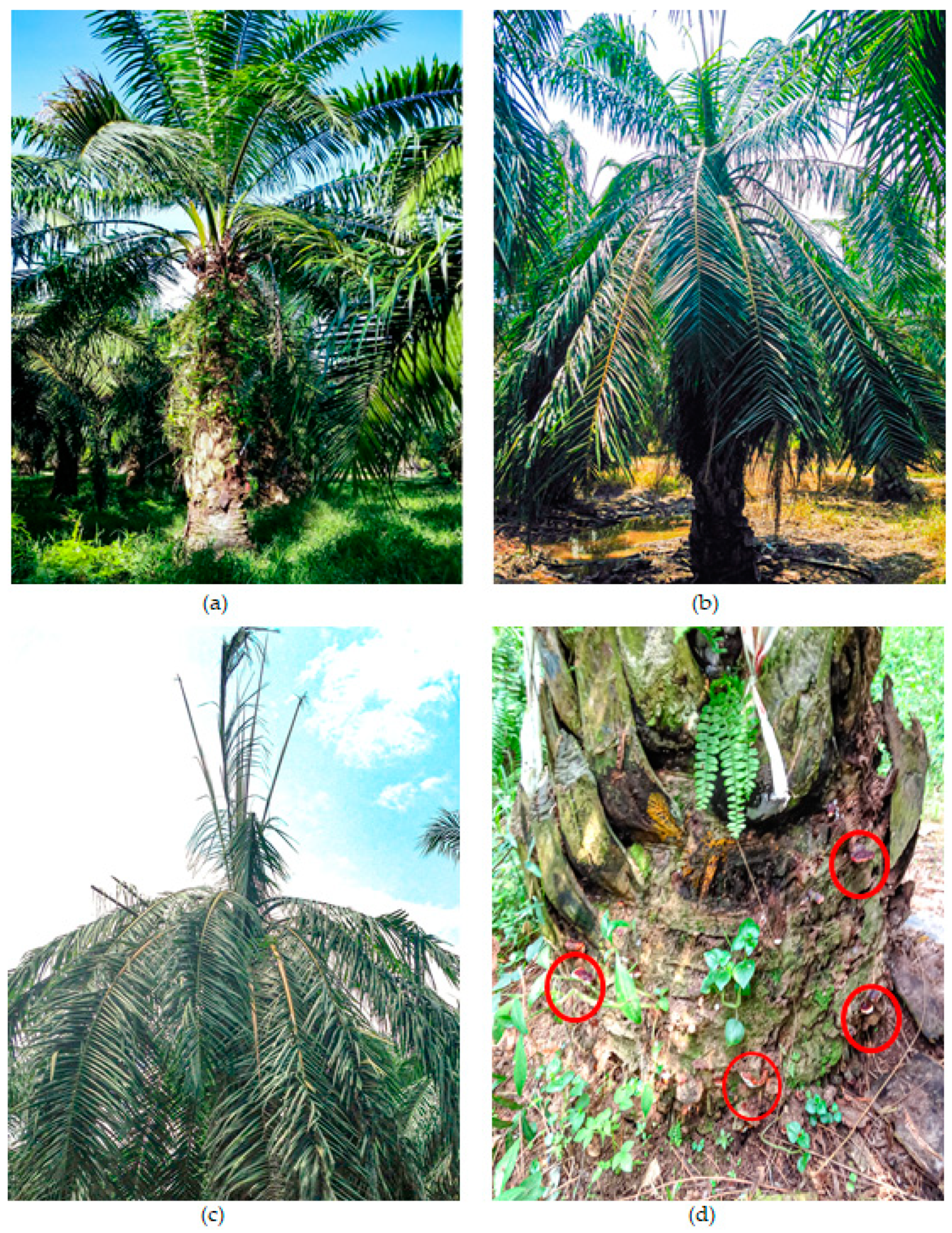
Field data collection was conducted on 20 March 2017. The census of oil palm trees that were non-infected and infected by G. boninense was obtained from the Malaysian Palm Oil Board (MPOB) and the infection status of the BSR disease was identified based on the visual symptoms stated by the expert, as shown in Table 1 and Figure 2. The GPS coordinates of individual trees were recorded using Trimble R6 GPS receiver (Trimble Navigation Limited, Sunnyvale, CA, USA) and the total number of oil palm trees that were non-infected and infected by G. boninense collected for this study were 55 and 37, respectively.

2.3. Dataset Description

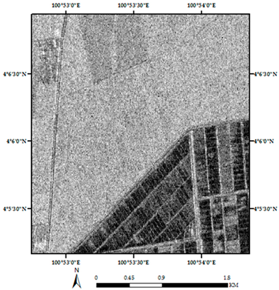
This study used ALOS PALSAR-2 image data archived on 20 March 2017. The scene observed and captured on ALOS PALSAR-2 is a fine beam dual polarization (HH and HV) and a high spatial resolution 10 m, with a pixel size of 6.25 m × 6.25 m and a 24 cm radar wavelength. Table 2 shows the specification of ALOS PALSAR-2 sensor data.

2.4. Data Analysis and Evaluation

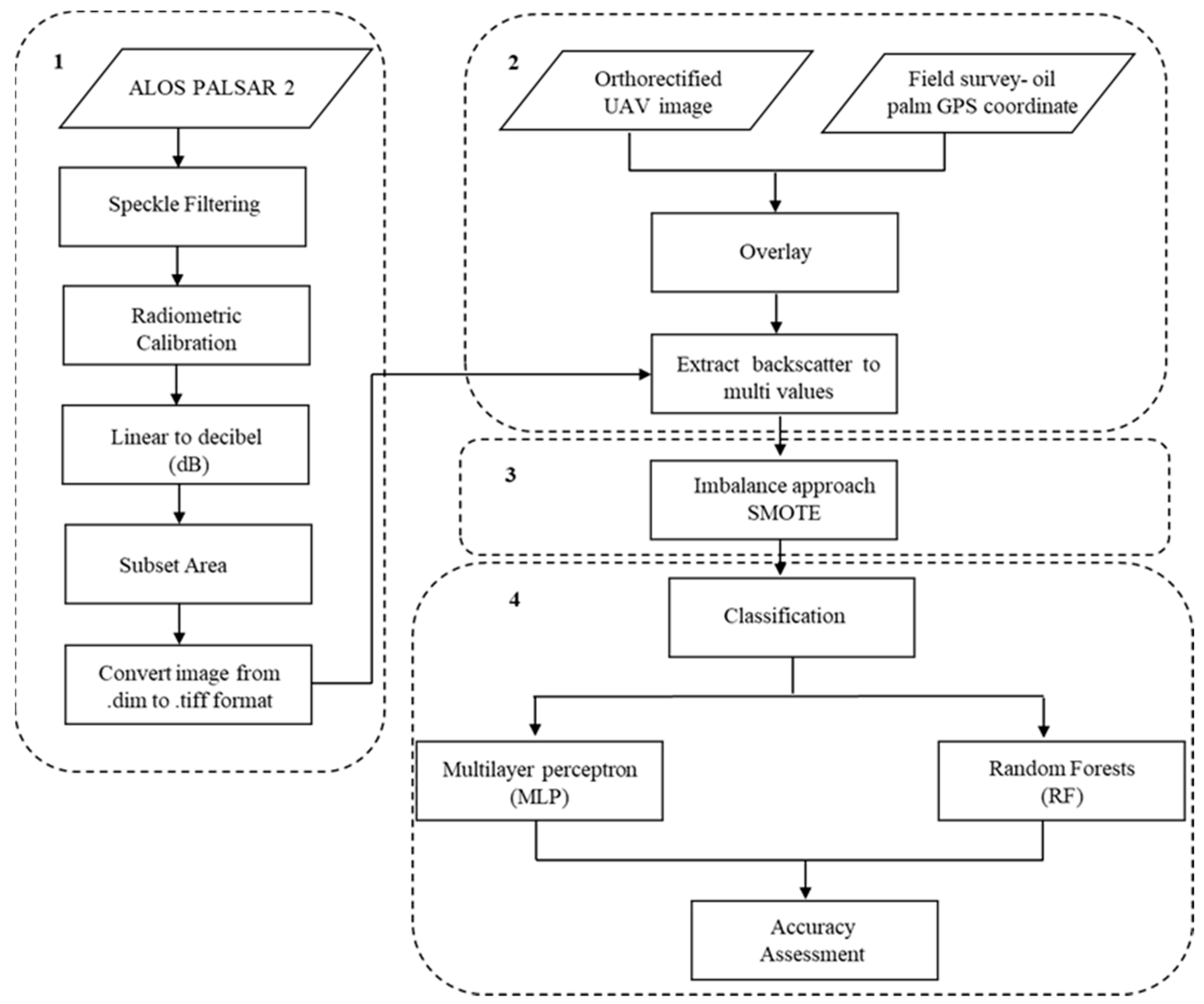
The four main steps involved in this research and the workflow of the processing are shown in Figure 3.

2.4.1. SAR Image Pre-Processing

As shown in Figure 3, ALOS PALSAR-2 data were first subjected to speckle filtering and radiometric correction. Since ALOS PALSAR-2 data are stored in Level 1.5 product, data have been subjected to geometrical correction; thus, terrain correction step was unnecessary for this data. To reduce high frequency noise in ALOS PALSAR-2 data, speckle filtering was applied to the image. Several well-known researchers have developed filtering algorithms for SAR images [48,49,50]. A wide range of filtering techniques was applied to varying researches. Reduction of speckle noise is one of the most important processes to increase the quality of coherent radar images. Image variance or speckle is a granular noise that inherently exists and degrades the quality of active radar and SAR images [51] found that Lee filter is best used for agricultural areas; hence, Lee filtering was adopted in this research. A filter’s Kernel size plays an important role in smoothing the image [52]. To preserve the details of the image, appropriate size should be selected for better results. The 7 × 7 of window filter size was utilized for HH and HV based on high Equivalent Number of Looks (ENL) values, and low Speckle Suppression and Mean Preservation Index (SMPI) value, so it indicates better performance in terms of speckle reduction and means preservation. Radiometric correction was then applied to the image to obtain the sigma naught value in the unit of decibel (dB), as in Equation (1) [53]
σ o = 10 × l o g 10 D N 2 83   d B
where DN is the digital number of the ALOS PALSAR-2 data.
Subsequently, the SAR image was subset into the region of interest, and the data image type was converted from the .dim format to the .tiff format prior to being processed using ArcGIS Desktop software version 10.6.1 (Environmental Systems Research Institute (ESRI), Redland, CA,USA).

2.4.2. Training Data

In the second step, an orthorectified UAV image (3DR Iris + drone with MAPIR Survey 2 camera (MAPIR, Peau Prodiuctions, Inc., San Diego, CA, USA), as a base map was overlaid with the GPS coordinate of each individual tree, which had been recorded using Trimble GPS device during the field survey. Afterwards, the SAR image and coordinate of each tree were overlaid to extract backscattering values. The backscattering value for each oil palm point was extracted from the processed SAR image by using Extract Multi Values tool in ArcGIS. As the SAR image was tested with dual polarization (HH and HV), each digitized point possessed two different backscatter values.

2.4.3. Imbalance Data Approach

In this study, data imbalance was an issue due to the small number of instances in the infected class compared to the non-infected. Therefore, the imbalance approach, SMOTE was applied for the classification of non-infected and infected by G.boninense. The algorithm was chosen because it is of low complexity, has less bias, and requires minimal computation [45,54]. From the SMOTE result, non-infected and infected by G. boninense, was pooled to represent the training and testing datasets with a 70:30 ratio, respectively.

Data Sampling

SMOTE is a technique that oversamples the minority class by generating synthetic examples [55]. SMOTE first randomly selects an example of a minority class and finds the nearest minority class neighbor. The synthetic instance is then created by choosing one of the k nearest neighbors b at random and connecting a and b to form a line segment in space characteristics. The synthetic samples are produced as a convex combination of two selected samples a and b [56]. Finally, the new instances of minority class are synthesized. In this study, SMOTE was executed using an open-source ML program, Waikato Environment for Knowledge Analysis (WEKA) version 3.8.5 [57]. Prior to the classification, the SMOTE parameters were tuned and summarized in Table 3.

2.4.4. Classification

The process of manipulating the backscatter of dual-polarization values can result in more effective classification [58]. Therefore, instead of using the original backscatter (HH and HV) polarization values, a trial was also made to obtain other variables gained from the backscatter of dual polarization values. The backscatter variables generated for this study were (i) range (HH-HV); (ii) average (HH + HV/2); and (iii) simple band ratio (HH/HV), (HV/HH). All six (6) backscatter variables were used in this study, as shown in Table 4. In this study, the variables of backscatter of dual-polarization values were used as the ML inputs as illustrated in Table 5.

Machine Learning Approach

The ML approach could also be used to classify a large number of samples and classify a smaller number of samples [60,61]. Due to the small number of samples, we performed a cross-validation process to evaluate model performance. The K-fold cross-validation function in WEKA was used to split the data into training and testing datasets and obtain an independent evaluation of the model accuracy. Thus, the resulting model was valid and not limited to only one set of data. Ten iterations of cross-validation were performed, where the original data were randomly partitioned into ten subsamples. Two ML methods were used, as described below:
(1) Multilayer Perceptron (MLP). MLP is an artificial neural network feed-forward model that charts input data sets to a set of appropriate outputs. An MLP is the result of multiple layers of nodes being connected to one another [62]. Every node is a neuron (or processing element) with a nonlinear activation function, except for the input nodes. For training the network, MLP utilizes a supervised learning technique called backpropagation [63]. MLP is a modification of the standard linear perception and can distinguish non-linearly separable data.
(2) Random Forests (RF). RF is a type of classification algorithm that contains a group of decision tree stochastics. In RF, the individual bootstrap sample is drawn from the original datasets to train each tree, and each node has a random feature from the original dataset [64]. The dataset is assigned according to the majority vote from the ensemble of trees built by the RF algorithm [65]. Moreover, it has high predictive accuracy, and it works well with an imbalanced dataset and robust against noise [66,67].

Accuracy Assessment

Overall accuracy as an assessment metric will be biased because of the data imbalance problem since it mainly represents the majority class’s accuracy [54]. This analysis, therefore, presented the description of the confusion matrix as an alternative in terms of the success rate of the non-infected and infected G. boninense, along with the balanced classification rate or balanced accuracy (BCR) and the receiver operating characteristics (ROC) curve region (AUC). These metrics were used to evaluate different classifier approaches and measure their performance. Following the classification of Kappa value by [68], we considered the BCR below 40.00% as poor, between 40.00% and 80.00% as moderate and above 80.00% as robust. While, the AUC value of 0.50 is regarded as fail, 0.51−0.69 is considered to be poor, 0.70–0.79 is deemed to be acceptable, 0.80–0.89 is considered excellent, and 0.90–1.00 is regarded as outstanding [69]. Finally, ANOVA and Tukey Honest Significant Difference (HSD) test at p < 0.05 using IBM SPSS Statistics for Windows, version 19 (IBM Corp., Armonk, NY, USA) determined the significance level of the differences between classifiers and backscatter variables.

3. Results

3.1. Sensitivity of Variables of Backscatter Used

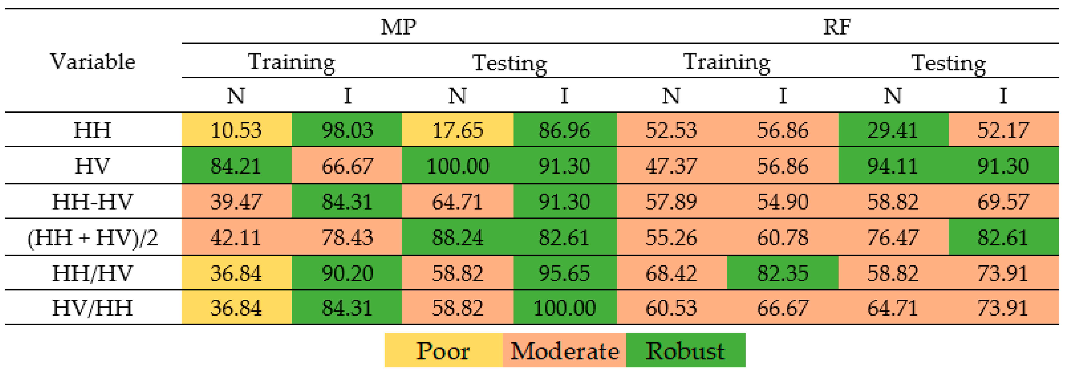
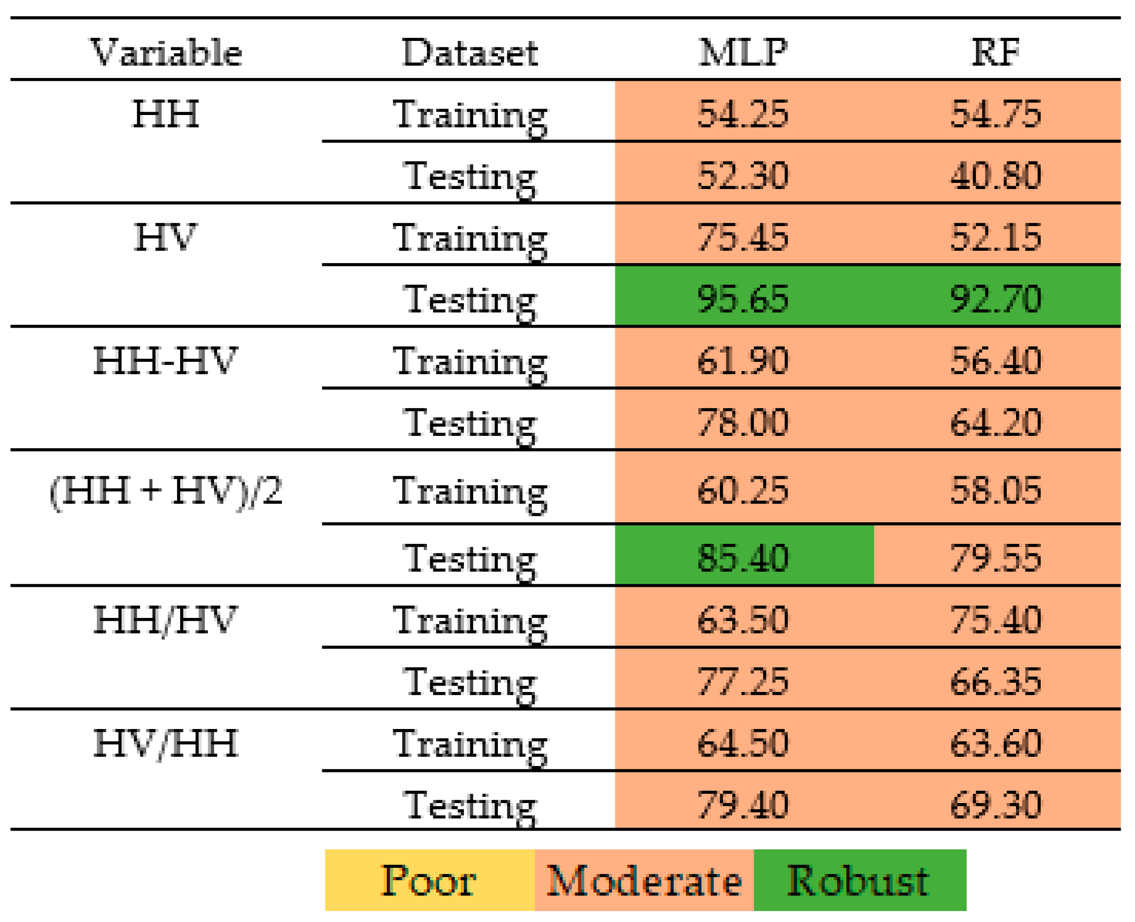
The success rate (%), BCR (%) and AUC of the non-infected and infected by G. boninense are illustrated in a heat map shown in Figure 4, Figure 5 and Figure 6, respectively. Since the accuracy assessment of training and testing datasets was about similar, the result and discussion of success rate, BCR and AUC are focused on the testing dataset. As shown in Figure 4, the MLP model performed better than the RF model, given any backscatter variables. HV had a higher correctly classified the G. boninense non-infected and infected oil palm trees for both classifiers in terms of backscatter variable. The MLP classifier model for the variable HV had a robust success rate with correctly classified 100% for non-infected and 91.30% for infected G. boninense, BCR 95.65% (robust) and AUC 0.92 (outstanding). Meanwhile, the RF classifier model for the variable HV had a robust success rate with correctly classified 94.11% for non-infected and 91.30% for infected G. boninense, BCR 92.70% (robust) and AUC 0.95 (outstanding).
Contrary to the HH variable, we correctly classified the G. boninense non-infected and infected oil palm trees for both classifiers. The MLP classifier model for the variable HH had a poor and robust success rate with correctly classified 17.65% for non-infected and 86.96% for infected G. boninense, BCR 52.30% (moderate) and AUC 0.49 (fail). Meanwhile, the RF classifier model for the variable HH had a poor to moderate success rate with correctly classified 29.41% for non-infected and 52.17% for infected G. boninense, BCR 40.80% (moderate) and AUC 0.44 (poor).
However, the manipulation results of the variables obtained in this study only reached higher from average variables ((HH + HV)/2). The MLP classifier model for the variable HH + HV)/2 had a robust success rate with correctly classified 88.24% for non-infected and 82.61% for infected G. boninense, BCR 85.40% (robust) and AUC 0.88 (excellent). Meanwhile, the RF classifier model for the variable HH + HV)/2 had a moderate to robust success rate with correctly classified 76.47% for non-infected and 82.61% for infected G. boninense, BCR 79.55% (moderate) and AUC 0.85 (excellent).
The ANOVA (Table 6) test demonstrated that there is no statistically significant difference between backscatter variables. However, a Tukey post hoc (Table 7) test showed that the HH and HV were statistically significant (p = 0.03) and there was no statistically significant difference between the other backscatter variables. The Tukey’s HSD (Table 8) test depicted the mean comparison of BCR (%) highest for HV = 70.65% and lowest for HH = 50.53%.

3.2. Effects of Classifiers on the Model Performance

Based upon the results in the study, the MLP model performed slightly better than the RF model, given any backscatter variables, with BCR ranging from 52.30 to 95.65% (moderate to robust), AUC = 0.49–0.92 (fail to outstanding), non-infected success rate = 17.65–100% (poor to robust) and infected success rate = 82.61–100% (robust) compared to 40.80 to 92.70% (moderate to robust), AUC = 0.44–0.95 (fail to outstanding), non-infected success rate = 29.41–94.11% (poor to robust) and infected success rate = 52.17–100% (moderate to robust).
From the results obtained, the excellent variable selection also plays a role in determining the performance model. Results for the HV polarized backscatter variables were found to be better than other backscatter variables based on the results of the success rate, balanced accuracy (BCR) and the receiver operating characteristics (ROC) curve region, (AUC) for both classifiers.
The ANOVA also concluded that there is no statistically significant difference in model performance (p = 0.271). The Tukey’s HSD test depicted the mean comparison of BCR (%) slightly higher for MLP model = 70.65% than RF model = 64.44%.

4. Discussion

4.1. Sensitivity of Variables of Backscatter Used

The current study was to identify the potential backscatter variables for the classification of the BSR disease in oil palm plants. Several studies have shown the efficiency of backscattering of SAR data sensitivity to plant conditions [25,26,27]. The radar backscattering from crops is sensitive to the crop canopy structure and the underlying soil condition [70]. As regards the polarization response, cross-polarized backscatter is found to be more sensitive than co-polarized backscatter. This is attributed to the depolarization due to multiple reflection of incoming signals inside the plant canopy. This is consistent with conclusions in the literature as mentioned above that HV polarization is more sensitive compared to HH polarization.
This study discovered the potential to assess the feasibility of backscatter variables from SAR data in classifying oil palm trees that are non-infected and infected by G. boninense and revealed prediction accuracy. The backscatter of HV polarization has greater success in correctly classifying G. boninense non-infected and infected oil palm trees for both classifiers. The MLP classifier model for the HV polarization has a robust success rate with correctly classifying 100% of the non-infected and 91.30% of the infected G. boninense, BCR 95.65% (robust) and AUC 0.92 (outstanding). Meanwhile, the RF classifier model for the HV polarization had a robust success rate with correctly classifying 94.11% of the non-infected and 91.30% of the infected G. boninense, BCR 92.70% (robust) and AUC 0.95 (outstanding).

4.2. Effects of Classifiers on the Model Performance

Based upon the BCR, AUC, success rate of non-infected and infected by G. boninense as well as the ANOVA, both the MLP-based models and the RF-based models have almost similar performance in classifying the oil palm trees. We need a thorough understanding of the output of these methods in order to make maximum use of each classification system.
There are two factors we can consider when choosing an algorithm. (1) Performance; when deciding the algorithm to use for classification or regression, the algorithm’s overall output is a significant determinant. Both MLP and RF are able to distinguish linear and nonlinear relationships and MLP systems have more significant potential for this [71]. (2) Robustness; when evaluating performance it is necessary to look at the robustness of the application rather than the consistency of the fitting [72]. Although the data were generated from the same database, they do not work well with new data. Such a condition is considered “overfitting” [73]. In this situation, the respective delegate does not comply with the existing protocol robustness, reflecting its generality. In this scenario, we reduce the chance of over generalization. These can be minimized by restricting the number of models that can be suggested by an algorithm. To do so, both MLP and RF can be used with advantages and disadvantages. In MLP, the number of hidden neurons and layers has a significant effect on the complexity of the model, as well as the amount of regularization used when optimizing the weights. RF allows us to change the size and number of trees, or the size and depth of individual trees, to fit the issue. Additionally, each of these methods can manage uncertainty and overfitting. MLP are stereotyped as being especially sensitive to inputs, which may contribute to tendencies towards deviations [74].
Many previous studies involved the comparison of these classifiers. Another research study deals with the prediction of carbon and nitrogen in the soil and how different fields have different amounts of these two elements [75]. The research compares MLP, RF and Gradient Boosted Machines (GBM) to see better results. The findings indicate that the results differed according to the kinds of data used. The RF model outperformed other models in most situations. Another research done based on the comparison of MLP and RF in predicting building energy usage, which is a numerical prediction rather than a category classification case [76]. The study found MLP performed significantly better than RF.
In reality, both techniques help with various aspects of applications. ML has found that no single algorithm can be useful in every situation. Thus, no single algorithm always performs better, and the results of an algorithm will differ significantly depending on the application and the size of the dataset. Hence, one can compare various learning algorithms’ outputs for a particular problem to find the best algorithm. It is also useful to construct ensembles of multiple models generated with different approaches to combine their strengths, thus reducing their weaknesses.

5. Conclusions

In this study, the backscatter values of oil palm trees were extracted using ALOS PALSAR-2 image data and divided into two level status: non-infected and infected by G. boninense. Six (6) backscatter variables were used, namely HH, HV, range (HH-HV), average (HH + HV/2), simple band ratio (HH/HV), and simple band ratio (HV/HH) to generate ML models for the prediction of the BSR disease. Two classifier models were used; MLP and RF. In terms of model performance, given any backscatter variables, the MLP model had a balanced accuracy (BCR) ranging from 52.30% to 95.65% compared to 40.80% to 92.70% for the RF model. Comparison between the MLP model and RF model for the receiver operating characteristics (ROC) curve region, (AUC) gave a range of 0.49–0.92 and 0.44–0.95, respectively, for the MLP and RF models.
Regarding the polarization response, certain variables such as the fact HV that captures the phenomena under study better, stand out more significantly. The cross-polarized backscatter (HV) was found to be more sensitive to crop canopy structure than co-polarization backscatter (HH), which is more susceptible to the surface. Due to that, the results of the success rate, a balanced accuracy (BCR) and the receiver operating characteristics (ROC) curve region, (AUC) become low if it involves HH polarization as a variable. Using the most significant variables, HV, the MLP model had a balanced accuracy (BCR) of 95.65% compared to 92.70% for the RF model. Comparison between MLP model and RF model for the receiver operating characteristics (ROC) curve region, (AUC) gave a value of 0.92 and 0.95, respectively, for the MLP and RF models.
In conclusion, by using only the HV polarization, both the MLP and RF can be used to predict BSR disease with a relatively high accuracy. The major benefit derived from this study is the potential of using SAR data and the imbalanced data approach to classify oil palm trees infected by G. boninense using ML techniques. In the future, studies with samples of different severity levels will be used to analyse backscatter characteristics and identify oil palm trees that have been infected with BSR disease.

Author Contributions

Conceptualization, I.C.H. and A.R.M.S.; methodology, I.C.H. and A.R.M.S.; software, I.C.H. and A.R.M.S.; validation, A.R.M.S.; formal analysis, I.C.H.; investigation, I.C.H.; resources, A.R.M.S., S.K.B.; F.M.M. and K.A.; data curation, I.C.H.; writing—original draft preparation, I.C.H.; writing—review and editing, A.R.M.S., and F.M.M.; supervision, A.R.M.S. All authors have read and agreed to the published version of the manuscript.

Funding

This research received no external funding.

Data Availability Statement

Restrictions apply to ALOS PALSAR-2 data. Data were obtained from the Japanese Space Agency (JAXA).

Acknowledgments

Thanks and appreciation to the Ministry of Higher Education Malaysia and Universiti Teknologi Mara, Perak Branch, for providing a scholarship and study leave to Izrahayu Che Hashim, which made this research possible. We would express our gratitude to Universiti Putra Malaysia for providing the research’s support and facilities. We also would express our appreciation to Japan Aerospace Exploration Agency (JAXA) for the ALOS PALSAR-2 data. Our appreciation and thanks to all agencies that provided the field site and the census for oil palms, including Felcra Berhad Seberang Perak 10 and Malaysian Palm Oil Board (MPOB).

Conflicts of Interest

The authors declare no conflict of interest.

References

  1. Varga, S. Essential Palm Oil Statistics 2017. Palm Oil Anal. 2017, 1, 4–26. [Google Scholar]
  2. Hushiarian, R.; Yusof, N.A.; Dutse, S.W. Detection and control of Ganoderma boninense: Strategies and perspectives. Springerplus 2013, 2, 1–12. [Google Scholar] [CrossRef] [Green Version]
  3. Roslan, A.; Idris, A.S. Economic Impact of Ganoderma Incidence on Malaysian Oil Palm Plantation–a Case Study in Johor. Oil Palm Ind. Econ. J. 2012, 12, 24–30. [Google Scholar]
  4. Lai, O.-M.; Tan, C.-P.; Akoh, C.C. Palm Oil: Production, Processing, Characterisation, and Uses; AOCS Press: Urbana, IL, USA, 2012; ISBN 9780981893693. [Google Scholar]
  5. Mohammed, C.L.; Rimbawanto, A.; Page, D.E. Management of basidiomycete root- and stem-rot diseases in oil palm, rubber and tropical hardwood plantation crops. For. Pathol. 2014, 44, 428–446. [Google Scholar] [CrossRef]
  6. Priwiratama, H.; Susanto, A. Utilization of Fungi for the Biological Control. of Insect Pests and Ganoderma Disease in the Indonesian Oil Palm Industry. J. Agric. Sci. Technol. 2014, 4, 103–111. [Google Scholar]
  7. Santoso, H.; Tani, H.; Wang, X. Random Forest classification model of basal stem rot disease caused by Ganoderma boninense in oil palm plantations. Int. J. Remote Sens. 2017. [Google Scholar] [CrossRef]
  8. Singh, G. Ganoderma—The scourge of oil palm in the coastal area. In Proceedings of the Ganoderma workshop, Bangi, Selangor, Malaysia, 11 September 1990; Palm Oil Research Institute of Malaysia: Kuala Lumpur, Malaysia, 1991; pp. 7–35. [Google Scholar]
  9. Turner, P.D. Oil Palm Diseases and Disorders; Oxford Univ. Press: Kuala Lumpur, Malaysia, 1981; ISBN 0195804686. [Google Scholar]
  10. Rahmahwati, R.; Zulkilfli, A.M.; Ramle, M. Factors Affecting Yield Achieved by Participants of the Quality Oil Palm Seedlings Assistance Scheme in Sabah and Sarawak. Oil Palm Ind. Econ. J. 2019, 19, 44–56. [Google Scholar]
  11. Khaled, A.Y.; Abd Aziz, S.; Bejo, S.K.; Nawi, N.M.; Seman, I.A.; Onwude, D.I. Early detection of diseases in plant tissue using spectroscopy–applications and limitations. Appl. Spectrosc. Rev. 2018, 53, 36–64. [Google Scholar] [CrossRef]
  12. Khosrokhani, M.; Khairunniza-Bejo, S.; Pradhan, B. Geospatial technologies for detection and monitoring of Ganoderma basal stem rot infection in oil palm plantations: A review on sensors and techniques. Geocarto Int. 2018, 33, 260–276. [Google Scholar] [CrossRef]
  13. Liaghat, S.; Ehsani, R.; Mansor, S.; Shafri, H.Z.M.; Meon, S.; Sankaran, S.; Azam, S.H.M.N. Early detection of basal stem rot disease (Ganoderma) in oil palms based on hyperspectral reflectance data using pattern recognition algorithms. Int. J. Remote Sens. 2014, 35, 3427–3439. [Google Scholar] [CrossRef]
  14. Shafri, H.Z.M.; Anuar, M.I.; Seman, I.A.; Noor, N.M. Spectral discrimination of healthy and ganoderma-infected oil palms from hyperspectral data. Int. J. Remote Sens. 2011, 32, 7111–7129. [Google Scholar] [CrossRef]
  15. Lelong, C.C.D.; Roger, J.M.; Brégand, S.; Dubertret, F.; Lanore, M.; Sitorus, N.A.; Raharjo, D.A.; Caliman, J.P. Evaluation of oil-palm fungal disease infestation with canopy hyperspectral reflectance data. Sensors 2010, 10, 734–747. [Google Scholar] [CrossRef] [PubMed]
  16. Shafri, H.Z.M.; Hamdan, N. Hyperspectral imagery for mapping disease infection in oil palm plantation using vegetation indices and red edge techniques. Am. J. Appl. Sci. 2009, 6, 1031–1035. [Google Scholar] [CrossRef] [Green Version]
  17. Santoso, H.; Gunawan, T.; Jatmiko, R.H.; Darmosarkoro, W.; Minasny, B. Mapping and identifying basal stem rot disease in oil palms in North Sumatra with QuickBird imagery. Precis. Agric. 2011, 12, 233–248. [Google Scholar] [CrossRef]
  18. Xie, Y.; Sha, Z.; Yu, M. Remote sensing imagery in vegetation mapping: A review. J. Plant Ecol. 2008, 1, 9–23. [Google Scholar] [CrossRef]
  19. Kakaes, K.; Greenwood, F.; Lippincot, M.; Dosemagen, S.; Meier, P.; Wich, S. Drones and Aerial Observation: New Technologies for Property Rights, Human Rights, and Global Development A Primer; New America: Washington, DC, USA, 2015. [Google Scholar]
  20. Al-Wassai, F.A.; Kalyankar, N.V. Image Fusion Technologies in Commercial Remote Sensing Packages. arXiv 2013, arXiv:1307.2440. [Google Scholar]
  21. Wang, D.; Su, Y.; Zhou, Q.; Chen, Z. Advances in research on crop identification using SAR. In Proceedings of the 2015 Fourth International Conference on Agro-Geoinformatics (Agro-Geoinformatics), Istanbul, Turkey, 20–24 July 2015; pp. 312–317. [Google Scholar] [CrossRef]
  22. Chakraborty, M.; Manjunath, K.R.; Panigrahy, S.; Kundu, N.; Parihar, J.S. Rice crop parameter retrieval using multi-temporal, multi-incidence angle Radarsat SAR data. ISPRS J. Photogramm. Remote Sens. 2005, 59, 310–322. [Google Scholar] [CrossRef]
  23. Shao, Y.; Fan, X.; Liu, H.; Xiao, J.; Ross, S.; Brisco, B.; Brown, R.; Staples, G. Rice monitoring and production estimation using multitemporal RADARSAT. Remote Sens. Environ. 2001, 76, 310–325. [Google Scholar] [CrossRef]
  24. Moran, M.S.; Inoue, Y.; Barnes, E.M. Opportunities and limitations for image-based remote sensing in precision crop management. Remote Sens. Environ. 1997, 61, 319–346. [Google Scholar] [CrossRef]
  25. Huang, W.; Sun, G.; Ni, W.; Zhang, Z.; Dubayah, R. Sensitivity of Multi-Source SAR Backscatter to Changes in Forest aboveground Biomass. Remote Sens. 2015, 7, 9587–9609. [Google Scholar] [CrossRef] [Green Version]
  26. Patel, P.; Srivastava, H.S.; Panigrahy, S.; Parihar, J.S. Comparative evaluation of the sensitivity of multi-spolarised multi-frequency SAR backscatter to plant density. Int. J. Remote Sens. 2006, 27, 293–305. [Google Scholar] [CrossRef]
  27. Srivastava, H.S.; Patel, P.; Navalgund, R.R. Application Potentials of Synthetic Aperture Radar Interferometry for Land-Cover Mapping and Crop-Height Estimation. Curr. Sci. 2006, 91, 783–788. [Google Scholar]
  28. Krapivin, V.F.; Varotsos, C.A.; Soldatov, V.Y. New Ecoinformatics Tools in Environmental Science: Applications and Decision-Making; Springer: Vienna, Austria, 2015; ISBN 9783319139784. [Google Scholar]
  29. Silva, W.F.; Rudorff, B.F.T.; Formaggio, A.R.; Paradella, W.R.; Mura, J.C. Simulated multipolarized MAPSAR images to distinguish agricultural crops. Sci. Agric. 2012, 69, 201–209. [Google Scholar] [CrossRef] [Green Version]
  30. Holmes, M.G. Monitoring vegetation in the future: Radar. Bot. J. Linn. Soc. 1992, 108, 93–109. [Google Scholar] [CrossRef]
  31. Chang, C.-W.; Lee, H.-W.; Liu, C.-H. A Review of Artificial Intelligence Algorithms Used for Smart Machine Tools. Inventions 2018, 3, 41. [Google Scholar] [CrossRef] [Green Version]
  32. Brodley, C.E.; Friedl, M.A. Decision tree classification of land cover from remotely sensed data. Remote Sens. Environ. 1997, 61, 399–409. [Google Scholar] [CrossRef]
  33. Qian, Y.; Zhou, W.; Yan, J.; Li, W.; Han, L.; Qian, Y.; Zhou, W.; Yan, J.; Li, W.; Han, L. Comparing Machine Learning Classifiers for Object-Based Land Cover Classification Using Very High Resolution Imagery. Remote Sens. 2014, 7, 153–168. [Google Scholar] [CrossRef]
  34. Chen, Y.; Dou, P.; Yang, X. Improving Land Use/Cover Classification with a Multiple Classifier System Using AdaBoost Integration Technique. Remote Sens. 2017, 9, 1055. [Google Scholar] [CrossRef] [Green Version]
  35. Guidici, D.; Clark, M. One-Dimensional Convolutional Neural Network Land-Cover Classification of Multi-Seasonal Hyperspectral Imagery in the San Francisco Bay Area, California. Remote Sens. 2017, 9, 629. [Google Scholar] [CrossRef] [Green Version]
  36. Stojanova, D.; Panov, P.; Gjorgjioski, V.; Kobler, A.; Džeroski, S. Estimating vegetation height and canopy cover from remotely sensed data with machine learning. Ecol. Inform. 2010, 5, 256–266. [Google Scholar] [CrossRef]
  37. Cho, M.A.; Mathieu, R.; Asner, G.P.; Naidoo, L.; van Aardt, J.; Ramoelo, A.; Debba, P.; Wessels, K.; Main, R.; Smit, I.P.J.; et al. Mapping tree species composition in South African savannas using an integrated airborne spectral and LiDAR system. Remote Sens. Environ. 2012, 125, 214–226. [Google Scholar] [CrossRef]
  38. Dalponte, M.; Frizzera, L.; Ørka, H.O.; Gobakken, T.; Næsset, E.; Gianelle, D. Predicting stem diameters and aboveground biomass of individual trees using remote sensing data. Ecol. Indic. 2018, 85, 367–376. [Google Scholar] [CrossRef]
  39. Lee, J.; Im, J.; Kim, K.; Quackenbush, L. Machine Learning Approaches for Estimating Forest Stand Height Using Plot-Based Observations and Airborne LiDAR Data. Forests 2018, 9, 268. [Google Scholar] [CrossRef] [Green Version]
  40. Shekoofa, A.; Emam, Y.; Shekoufa, N.; Ebrahimi, M.; Ebrahimie, E. Determining the most important physiological and agronomic traits contributing to smaise grain yield through machine learning algorithms: A new avenue in intelligent agriculture. PLoS ONE 2014, 9, e97288. [Google Scholar] [CrossRef] [Green Version]
  41. Lillo-Saavedra, M.F.; Gonzalo-Martín, C.; García-Pedrero, A.; Rodriguéz-Esparragón, D. A random forest and superpixels approach to sharpen thermal infrared satellite imagery. In Remote Sensing for Agriculture, Ecosystems, and Hydrology XIX; Neale, C.M., Maltese, A., Eds.; SPIE: Bellingham, DC, USA, 2007; Volume 10421, p. 104210H. [Google Scholar]
  42. Liakos, K.G.; Busato, P.; Moshou, D.; Pearson, S.; Bochtis, D. Machine learning in agriculture: A review. Sensors 2018, 18, 1–29. [Google Scholar] [CrossRef] [Green Version]
  43. Rumpf, T.; Mahlein, A.K.; Steiner, U.; Oerke, E.C.; Dehne, H.W.; Plümer, L. Early detection and classification of plant diseases with Support Vector Machines based on hyperspectral reflectance. Comput. Electron. Agric. 2010, 74, 91–99. [Google Scholar] [CrossRef]
  44. Ur Rahman, H.; Ch, N.J.; Manzoor, S.; Najeeb, F.; Siddique, M.Y.; Khan, R.A. A Comparative Analysis of Machine Learning Approaches for Plant Disease Identification. Adv. Life Sci. 2017, 4, 120–126. [Google Scholar]
  45. Thabtah, F.; Hammoud, S.; Kamalov, F.; Gonsalves, A. Data imbalance in classification: Experimental evaluation. Inf. Sci. 2020, 513, 429–441. [Google Scholar] [CrossRef]
  46. Chemchem, A.; Alin, F.; Krajecki, M. Combining SMOTE sampling and machine learning for forecasting wheat yields in France. In Proceedings of the IEEE 2nd International Conference on Artificial Intelligence and Knowledge Engineering, AIKE, Sardinia, Italy, 3–5 June 2019; Institute of Electrical and Electronics Engineers Inc.: Piscataway, NJ, USA, 2019; pp. 9–14. [Google Scholar]
  47. Ma, H.; Huang, W.; Jing, Y.; Yang, C.; Han, L.; Dong, Y.; Ye, H.; Shi, Y.; Zheng, Q.; Liu, L.; et al. Integrating growth and environmental parameters to discriminate powdery mildew and aphid ofwinter wheat using bi-temporal Landsat-8 imagery. Remote Sens. 2019, 11, 846. [Google Scholar] [CrossRef] [Green Version]
  48. Lee, J. Sen Digital Image Enhancement and Noise Filtering by Use of Local Statistics. IEEE Trans. Pattern Anal. Mach. Intell. 1980, PAMI-2, 165–168. [Google Scholar] [CrossRef] [PubMed] [Green Version]
  49. Frost, V.S.; Stiles, J.A.; Shanmugan, K.S.; Holtzman, J.C. A Model for Radar Images and Its Application to Adaptive Digital Filtering of Multiplicative Noise. IEEE Trans. Pattern Anal. Mach. Intell. 1982, PAMI-4, 157–166. [Google Scholar] [CrossRef] [PubMed]
  50. Kuan, D.T.; Sawchuk, A.A.; Strand, T.C.; Chavel, P. Adaptive Noise Smoothing Filter for Images with Signal-Dependent Noise. IEEE Trans. Pattern Anal. Mach. Intell. 1985, PAMI-7, 165–177. [Google Scholar] [CrossRef] [PubMed]
  51. Ozdarici, A.; Akyurek, Z. A Comparison of Sar Filtering Techniques on Agricultural Area Identification. In Proceedings of the ASPRS 2010 Annual Conference, San Diego, CA, USA, 26–30 April 2010; pp. 26–30. [Google Scholar]
  52. Mahdavi, S.; Salehi, B.; Moloney, C.; Huang, W.; Brisco, B. Speckle filtering of Synthetic Aperture Radar images using filters with object-size-adapted windows. Int. J. Digit. Earth 2018, 11, 703–729. [Google Scholar] [CrossRef]
  53. Rosenqvist, A.; Shimada, M.; Ito, N.; Watanabe, M. ALOS PALSAR: A pathfinder mission for global-scale monitoring of the environment. IEEE Trans. Geosci. Remote Sens. 2007, 45, 3307–3316. [Google Scholar] [CrossRef]
  54. Ryan Hoens, T.; Chawla, N.V. Imbalanced datasets: From sampling to classifiers. Imbalanced Learn. Found. Algorithms Appl. 2013, 43–59. [Google Scholar] [CrossRef]
  55. Chawla, N.V.; Bowyer, K.W.; Hall, L.O.; Kegelmeyer, W.P. SMOTE: Synthetic minority over-sampling technique. J. Artif. Intell. Res. 2002, 16, 321–357. [Google Scholar] [CrossRef]
  56. He, H.; Garcia, E.A. Learning from imbalanced data. IEEE Trans. Knowl. Data Eng. 2009, 21, 1263–1284. [Google Scholar] [CrossRef]
  57. Frank, E.; Hall, M.; Holmes, G.; Kirkby, R.; Pfahringer, B.; Witten, I.H.; Trigg, L. Weka-A Machine Learning Workbench for Data Mining. In Data Mining and Knowledge Discovery Handbook; Springer: Boston, MA, USA, 2009; pp. 1269–1277. [Google Scholar]
  58. Sarker, M.L.R.; Nichol, J.; Ahmad, B.; Busu, I.; Rahman, A.A. Potential of texture measurements of two-date dual polarization PALSAR data for the improvement of forest biomass estimation. ISPRS J. Photogramm. Remote Sens. 2012, 69, 146–166. [Google Scholar] [CrossRef]
  59. Omar, H.; Hamzah, K.A.; Ismail, M.H. The use of spolarised L-Band alos palsar for identifying forest cover in Peninsular Malaysia. In Proceedings of the 33rd Asian Conference on Remote Sensing, Pattaya, Thailand, 26–30 November 2012; Volume 1, pp. 263–272. [Google Scholar]
  60. Vabalas, A.; Gowen, E.; Poliakoff, E.; Casson, A.J. Machine learning algorithm validation with a limited sample size. PLoS ONE 2019, 14, e0224365. [Google Scholar] [CrossRef]
  61. Husin, N.A.; Khairunniza-Bejo, S.; Abdullah, A.F.; Kassim, M.S.M.; Ahmad, D.; Aziz, M.H.A. Classification of Basal Stem Rot Disease in Oil Palm Plantations Using Terrestrial Laser Scanning Data and Machine Learning. Agronomy 2020, 10, 1624. [Google Scholar] [CrossRef]
  62. Marius, P.; Balas, V.E.; Mastorakis, N.E.; Popescu, M.-C.; Balas, V.E. Multilayer Perceptron and Neural networks. WSEAS Trans. Circuits Syst. 2009, 8, 579–588. [Google Scholar]
  63. Stańczyk, U. Rough set and artificial neural network approach to computational stylistics. Smart Innov. Syst. Technol. 2013, 13, 441–470. [Google Scholar] [CrossRef]
  64. Immitzer, M.; Atzberger, C.; Koukal, T. Tree Species Classification with Random Forest Using very High Spatial Resolution 8-Band WorldView-2 Satellite Data. Remote Sens. 2012, 4, 2661–2693. [Google Scholar] [CrossRef] [Green Version]
  65. Berhane, T.; Lane, C.; Wu, Q.; Autrey, B.; Anenkhonov, O.; Chepinoga, V.; Liu, H. Decision-Tree, Rule-Based, and Random Forest Classification of High-Resolution Multispectral Imagery for Wetland Mapping and Inventory. Remote Sens. 2018, 10, 580. [Google Scholar] [CrossRef] [PubMed] [Green Version]
  66. Breiman, L. Random Forests. Mach. Learn. 2001, 45, 5–32. [Google Scholar] [CrossRef] [Green Version]
  67. Rodriguez-Galiano, V.F.; Ghimire, B.; Rogan, J.; Chica-Olmo, M.; Rigol-Sanchez, J.P. An assessment of the effectiveness of a random forest classifier for land-cover classification. ISPRS J. Photogramm. Remote Sens. 2012, 67, 93–104. [Google Scholar] [CrossRef]
  68. Jensen, J.R. Introductory digital image processing: A remote sensing perspective. Introd. Digit. image Process. Remote Sens. Perspect. 1996, 2, 65. [Google Scholar] [CrossRef]
  69. Hosmer, D.W.; Lemeshow, S. Assessing the Fit of the Model; Wiley: Hoboken, NJ, USA, 2000; pp. 143–202. [Google Scholar]
  70. Lopez-Sanchez, J.M.; Cloude, S.R.; Ballester-Berman, J.D. Rice phenology monitoring by means of SAR polarimetry at X-band. IEEE Trans. Geosci. Remote Sens. 2012, 50, 2695–2709. [Google Scholar] [CrossRef]
  71. You, H.; Ma, Z.; Tang, Y.; Wang, Y.; Yan, J.; Ni, M.; Cen, K.; Huang, Q. Comparison of ANN (MLP), ANFIS, SVM, and RF models for the online classification of heating value of burning municipal solid waste in circulating sfluidised bed incinerators. Waste Manag. 2017, 68, 186–197. [Google Scholar] [CrossRef] [PubMed]
  72. McPhail, C.; Maier, H.R.; Kwakkel, J.H.; Giuliani, M.; Castelletti, A.; Westra, S. Robustness Metrics: How Are They Calculated, When Should They Be Used and Why Do They Give Different Results? Earth’s Future 2018, 6, 169–191. [Google Scholar] [CrossRef]
  73. Ying, X. An Overview of Overfitting and its Solutions. J. Phys. Conf. Ser. 2019, 1168, 022022. [Google Scholar] [CrossRef]
  74. Dunne, R.A. A Statistical Approach to Neural Networks for Pattern Recognition; John Wiley & Sons, Inc.: Hoboken, NJ, USA, 2007; ISBN 9780470148150. [Google Scholar]
  75. Nawar, S.; Mouazen, A. Comparison between Random Forests, Artificial Neural Networks and Gradient Boosted Machines Methods of On-Line Vis-NIR Spectroscopy Measurements of Soil Total Nitrogen and Total Carbon. Sensors 2017, 17, 2428. [Google Scholar] [CrossRef]
  76. Ahmad, M.W.; Mourshed, M.; Rezgui, Y. Trees vs Neurons: Comparison between random forest and ANN for high-resolution prediction of building energy consumption. Energy Build. 2017, 147, 77–89. [Google Scholar] [CrossRef]
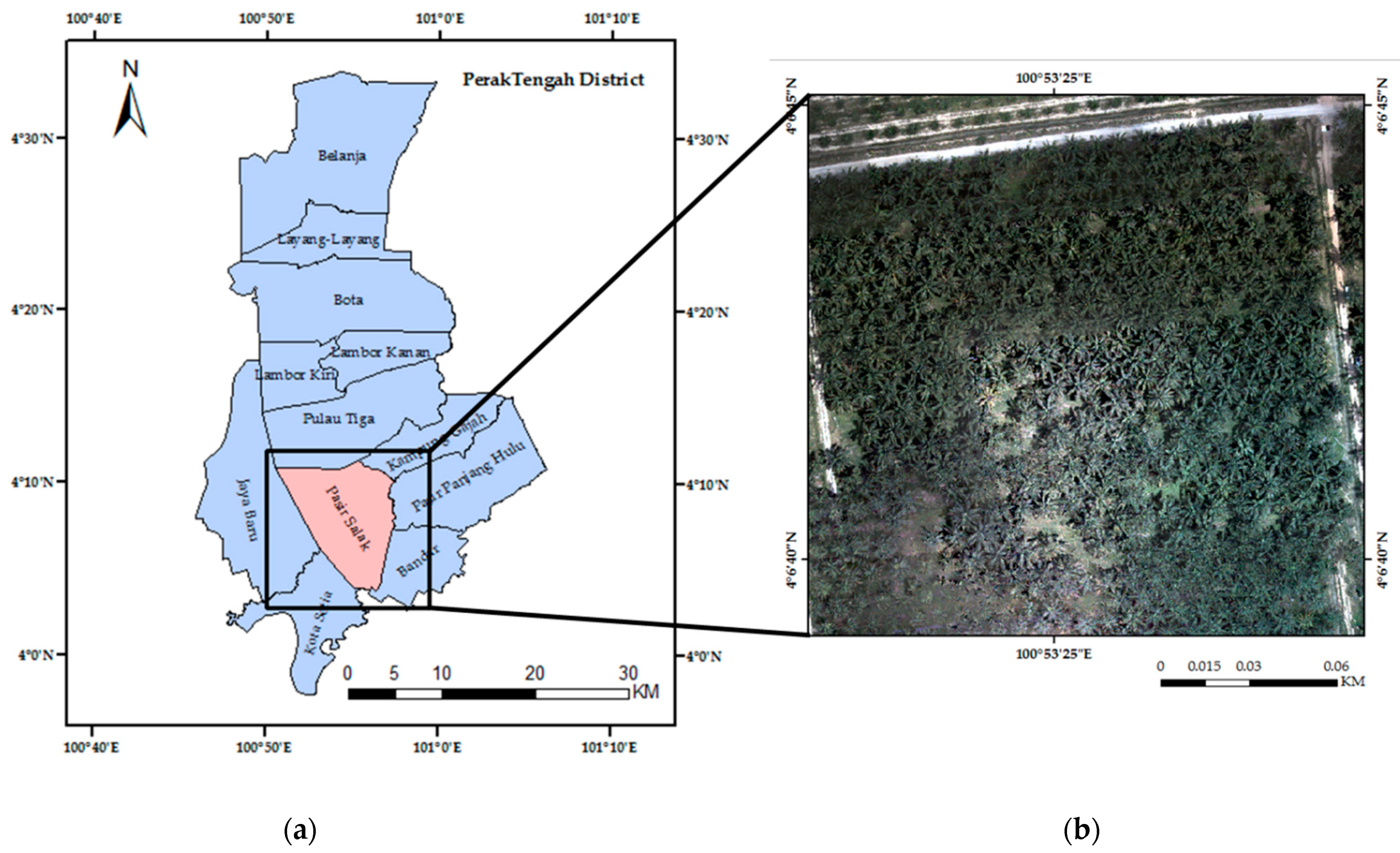
Figure 1. The Perak Tengah district, Perak, (a) Mukim Pasir Salak, (b) the image of the study area. The sample selection of oil palm trees with non-infected and infected by G. boninense is random based on census obtained from Malaysian Palm Oil Board (MPOB).
Agronomy 11 00532 g001
Figure 2. Oil palm trees in Felcra Seberang Perak 10, Phase 1, Parcel 3—(a) tree non-infected by G. boninense; (b) tree infected by G. boninense: showing foliar symptom such as the lower parts of leaves have formed like skirting; (c) tree infected by G. boninense: showing multiple unopened spears; (d) tree infected by G. boninense: showing the fruiting bodies and decay of the palm bole.
Agronomy 11 00532 g002
Figure 3. Research workflow—(1) SAR image pre-processing; (2) extraction of all pixel values for oil palm trees based on census data; (3) imbalanced data approach; and (4) classification of trees that were non-infected and infected by G.boninense in the study area.
Agronomy 11 00532 g003
Figure 4. The success rate (%) of non-infected (N) and infected (I) by G. boninense for variables of backscatter used.
Agronomy 11 00532 g004
Figure 5. The balanced accuracy (BCR) rate (%) of multilayer perceptron (MLP) and random forests (RF) classifier according to backscatter variables.
Agronomy 11 00532 g005
Figure 6. The area under the curve (AUC) of the MLP and RF classifier according to backscatter variables.
Agronomy 11 00532 g006
Table 1. Category and description of infection status of the oil palm trees.
CategoryDescription
Non-infectedHealthy palm, no foliage symptom (0%), no fruiting body
InfectedFoliage symptom more than 25%, produce fruiting bodies
Table 2. Details specification and image view of ALOS PALSAR-2.
ALOS PALSAR-2 SpecificationALOS PALSAR-2 Image View
Observation ModeStrip Map/High Resolution
Calibration Factor−83 Agronomy 11 00532 i001
Spatial Resolution10 m
Pixel Spacing6.25 m (2 looks)
Observation width70 km
Product Processed Level1.5
Range Resolution9.1 m
Azimuth Resolution5.3 m
PolarizationHH, HV (Fine Beam Dual Polarization)
Wavelength0.242 m (24 cm)
Off Nadir angle36.6°
Incident angle at centre scene40.55°
Table 3. Summary of the parameters used for the imbalance approach.
TechniqueParameter
SMOTEnearestNeighbors = 5
percentage = 100
Table 4. Variables used to classify trees that were non-infected and infected by G. boninense (Adapted from [59]).
VariableDescription
HHPixels values of original backscattering (dB) from HH polarization
HVPixels values of original backscattering (dB) from HV polarization
HH-HVRange generation by subtraction HH to HV polarizations (unitless)
(HH + HV)/2Average of HH and HV polarization (unitless)
HH/HVSimple ratio generation by dividing HH to HV polarizations (unitless)
HV/HHSimple ratio generation by dividing HV to HH polarizations (unitless)
Table 5. Descriptive statistics of variables gained from the backscatter of dual polarization values.
VariableDatasetStatusnMeanSDMinMax
HHTrainingNon-Infected38−11.372.42−16.70−4.91
Infected51−11.811.60−17.06−8.95
TestingNon-Infected17−11.132.31−15.78−6.49
Infected23−11.661.54−15.57−9.19
HVTrainingNon-Infected38−19.312.10−23.63−15.05
Infected51−17.422.38−22.25−11.51
TestingNon-Infected17−21.013.24−28.84−17.55
Infected23−16.102.12−21.43−10.99
HH-HVTrainingNon-Infected387.943.352.4516.32
Infected515.612.711.1513.00
TestingNon-Infected179.884.722.432.43
Infected234.602.15−1.598.07
(HH + HV)/2TrainingNon-Infected38−15.341.53−18.83−13.07
Infected51−14.641.51−19.44−12.05
TestingNon-Infected17−16.071.54−19.20−13.85
Infected23−13.941.56−18.65−18.65
HH/HVTrainingNon-Infected380.600.150.230.85
Infected510.690.120.411.02
TestingNon-Infected170.550.160.290.87
Infected230.720.130.581.15
HV/HHTrainingNon-Infected381.800.581.184.33
Infected511.500.280.962.45
TestingNon-Infected171.991.991.163.46
Infected231.410.200.870.87
Table 6. ANOVA for the effect of classifiers and backscatter variables on BCR (%).
SourceSum of SquaresdfMean SquareFSig.
Classifiers231.8821231.8821.2740.271
Backscatter Variables1797.4785359.4962.6540.057
Corrected Total2029.3606
Table 7. Multiple comparisons of backscatter variables on BCR (%) obtained from Tukey’s honest significant difference (HSD) test.
(I) Backscatter Variables(J) Backscatter VariablesMean Difference (I–J)Std. ErrorSig.95% Confidence Interval
Lower BoundUpper Bound
HHHV28.468.230.03−54.61−2.31
HH-HV14.608.230.51−40.7511.55
(HH + HV)/220.298.230.19−46.445.86
HH/HV20.108.230.19−46.256.05
HV/HH18.688.230.26−44.837.48
HVHH28.468.230.032.3154.61
HH-HV13.868.230.56−12.2940.01
(HH + HV)/28.188.230.91−17.9834.33
HH/HV8.368.230.91−17.7934.51
HV/HH9.798.230.84−16.3635.94
HH-HVHH14.608.230.51−11.5540.75
HV13.868.230.56−40.0112.29
(HH + HV)/2−5.698.230.98−31.8420.46
HH/HV−5.508.230.98−31.6520.65
HV/HH−4.088.231.00−30.2322.08
(HH+HV)/2HH20.298.230.19−5.8646.44
HV−8.188.230.91−34.3317.98
HH-HV5.698.230.98−20.4631.84
HH/HV0.198.231.00−25.9626.34
HV/HH1.618.231.00−24.5427.76
HH/HVHH20.108.230.19−6.0546.25
HV−8.368.230.91−34.5117.79
HH-HV5.508.230.98−20.6531.65
(HH + HV)/2−0.198.231.00−26.3425.96
HV/HH1.438.231.00−24.7327.58
HV/HHHH18.688.230.26−7.4844.83
HV−9.798.230.84−35.9416.36
HH-HV4.088.231.00−22.0830.23
(HH + HV)/2−1.618.231.00−27.7624.54
HH/HV−1.438.231.00−27.5824.73
Table 8. Mean comparison of BCR (%) obtained from Tukey’s HSD test according to classifiers and backscatter variables.
GroupMean (%)
ClassifiersMLP70.65
RF64.44
Backscatter VariablesHH50.53
HV78.99
HH-HV65.13
(HH + HV)/270.81
HH/HV70.63
HV/HH69.20
Publisher’s Note: MDPI stays neutral with regard to jurisdictional claims in published maps and institutional affiliations.