Prediction of Rice Yield in East China Based on Climate and Agronomic Traits Data Using Artificial Neural Networks and Partial Least Squares Regression

Abstract

Rice yield is not only influenced by factors of varieties and managements, but also by environmental factors. In this study, agronomic trait data of rice and climate data in eastern China were collected, and rice yields were predicted using a variety of algorithms, including the non-linear tool of feed-forward backpropagation neural networks (FFBN) and the linear model of partial least squares regression (PLSR). The results showed that both the agronomic traits and the climate data were significantly related with rice yield. The PLSR model showed that covariates occurred among the parameters, and modifications should be considered for climate data-based modelling. The FFBN model demonstrated better prediction performance than that of PLSR, in which the relation coefficient (R²) and root mean square error (RMSE) were 0.611 vs. 0.374 and 0.578 vs. 0.865 ton/ha using climate data, respectively; and 0.742 vs. 0.689 and 0.556 vs. 0.608 using agronomic trait data, respectively. When using fused data the R² and RMSE improved to 0.843 vs. 0.746 and 0.440 vs. 0.549, respectively. The optimum architecture of the FFBN consisted of one hidden layer with 29 neurons. Therefore, the FFBN algorithm is an effective option for the prediction of rice yield in complex systems of rice production.

1. Introduction

Rice (Oryza sativa L.) is a staple food for almost half of the world’s population [1], and 3.5 billion people depend on it for more than one-fifth of their daily calorie intake [2]. In China, rice accounts for 40% of the total calorie intake [3]. Thus, predicting the yield of the rice crop is important for food security. Rice grows in a wide range of environments and is productive in many situations where other crops would fail [2]. Both agricultural management and environmental factors play important roles in the yields of crops. Predicting the yield is not only highly important in field planning, decision making, stockholding, and risk management, but also provides a reference for agronomic policymakers to meet the challenge of national food security issues [4]. Therefore, effective and economical models are needed to predict the rice yield.

Field measurements, which are time consuming and expensive, are often used to evaluate the rice yield. However, the result of the rice yield from the harvest does not allow timely coping strategies to be implemented by policymakers. Therefore, many models have been created to solve this problem. Crop growth models based on biophysical parameters, which consist of genotypes, weather, soil conditions, and crop management approaches, have been applied not only to estimate the yield, but also to provide suggestions for crop yield management [4]. Prediction models using various data sources, such as remote sensing data, climate data, soil data, and agronomy traits, have been successfully used to predict the rice yield, and experimental data from remote systems and environmental data from local climate stations can be used for the prediction [5]. Son et al. used Moderate Resolution Imaging Spectroradiometer (MODIS)Normalized Difference Vegetation Index (NDVI) data to effectively predict the rice yield [4]. Agronomy traits were used to predict the yield of safflower [6] and sesame [7]. Online soil data and satellite images were also used to examine the variation of wheat yield [8], in which three different models were used to compare the responses of the crop yield to soils and land management [9].

In recent decades, various yield prediction models, including linear and non-linear models, have been developed. Linear and quadratic regression models have been applied to examine the response of crop yield to NDVI and Enhanced Vegetation Index (EVI) [10,11,12,13,14]. However, linear models are unstable in complex crop production systems. Therefore, many studies have applied non-linear models that can reliably estimate yield. Various algorithms, such as machine learning (ML) algorithms, random forests (RFs), decision trees, artificial neural networks (ANNs), and support vector machines (SVMs), have been applied to modeling non-linear relationships among variables [15,16,17,18]. ML showed a good performance for large and complex multi-dimensional datasets, and was able to learn the trends and patterns of data based on large amounts of data. These algorithms have been applied in many fields [19,20,21,22,23,24,25]. A recent study has shown that WOFOST-GTC, an improved model based on the World Food Studies model, is also suitable for estimating winter rapeseed production and oil quality under different scenarios [26]. Using an ANN to predict the adsorption in a rotating package bed (RPB), Li et al. found that ANN models have superior performance, accurate prediction, and more generalized ability than multiple nonlinear regression models [21]. The performance of ANN models in predicting ajowan production was found to be better than that of multiple linear regression [27]. Artificial neural network-based methods, widely used for predicting crop yields, have been used with high accuracy in different fields. However, the modeling effects of linear and non-linear algorithms, and the contributions of parameters to the rice yield, remain unclear in the main rice production areas of China.

In this study, back propagation neural networks (BPNNs) and partial least squares regression (PLSR) were applied to predict the rice yield in eastern China. The objectives of the study were: (1) to assess the performance of models applied to rice production with different databases, and (2) to optimize the prediction models, including the models of BPNN and PLSR, to guide applications in practice.

2. Materials and Methods

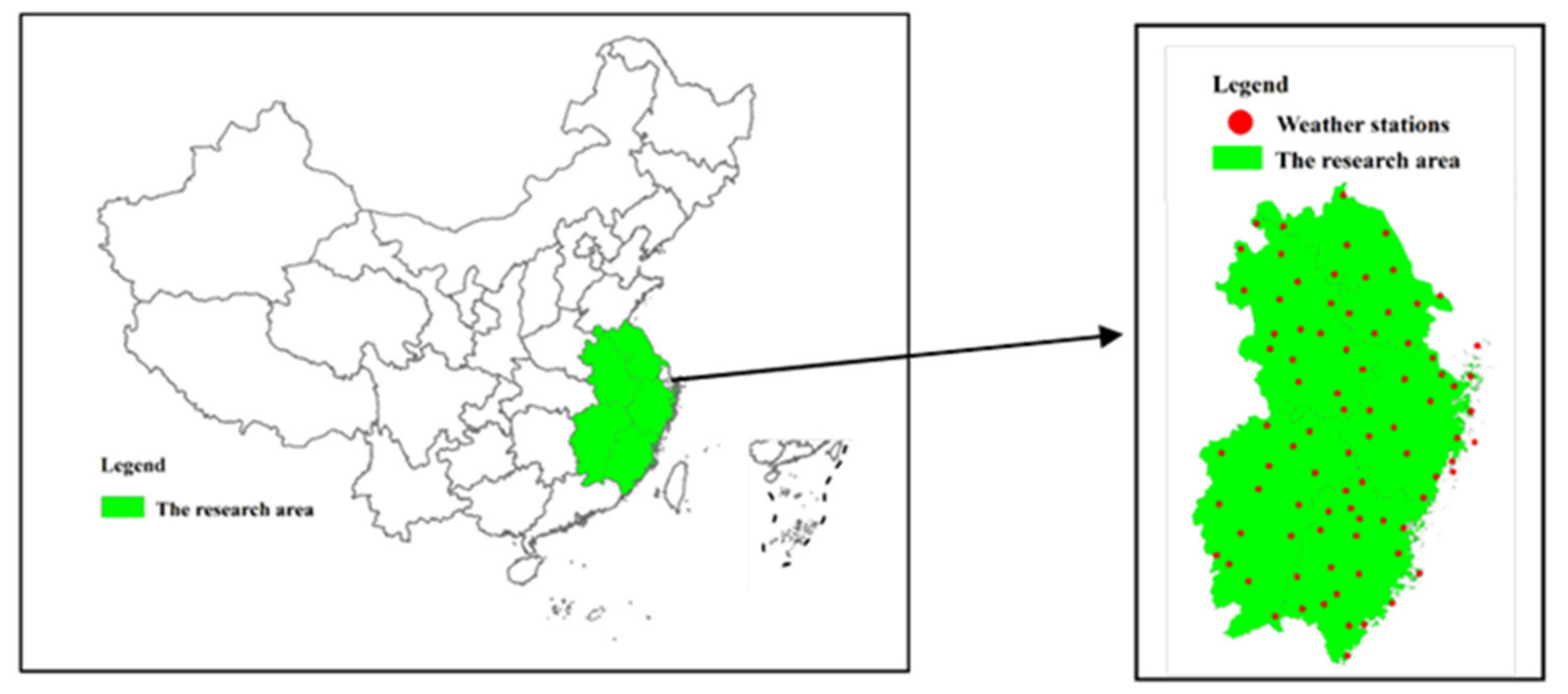
2.1. Data Collection

The main research area was in eastern China, where rice is mainly cultivated (Figure 1) with the typical paddy soil (anthrosol). A dataset including 979 records, consisting of weather and seed data, was used to build the prediction models. The database was randomly divided into training and testing sets, in which the training set contained 70% of the dataset, and the testing set contained the remaining 30%.

Weather data (daily temperature, daily precipitation, wind speed, sunshine duration, ground surface temperature, pressure, evaporation, solar radiation, and relative humidity) were acquired from the Greenhouse data share platform (http://data.sheshiyuanyi.com). The location of each weather station was entered in a geographic information system and overlaid with a map of China (Figure 1).

The seed’s agronomic trait data were obtained from the China seed industry big data platform (http://202.127.42.145). In the study area, the suitable rice varieties and specific agronomic traits were collected to form the dataset for building the prediction models. The agronomic traits are shown in

Table 1. Statistics of collected data.

	Variables	Synonym	Min	Max	Mean	Std
Agronomic Traits	Plant height (cm)	PH	75.10	143.5	106.9	14.43
	Effective panicle number (ten thousands/hm2)	EPN	160.5	441.0	276.2	49.67
	Filled grains per panicle (grains)	FGPP	73.90	273.70	143.60	43.21
	Seed set rate (%)	SSR	0.66	0.95	0.84	0.05
	Growth period (day)	GP	105.1	179.5	133.1	15.22
ClimateData	Ground surface temperature (°C)	GST	17.25	23.53	20.18	1.54
	Pressure of the station (hPa)	PRS	983.3	1015.5	999.4	9.31
	Relative humidity (%)	RHU	69.32	81.35	75.56	2.87
	Temperature (°C)	TEM	15.24	20.40	17.71	1.40
	Wind speed (m/s)	WIN	1.37	3.30	2.15	0.45
	Evaporation (mm)	EVP	1.63	3.60	2.53	0.38
	Precipitation (mm)	PRE	2.47	6.86	4.45	1.06
	Solar radiation (MJ/m2)	SR	9.83	22.03	13.71	2.26
	Sunshine duration (hour)	SSD	4.04	6.20	4.84	0.49
Rice Yield	Rice yield (ton/ha)	YIELD	5.07	11.30	8.48	1.11

.

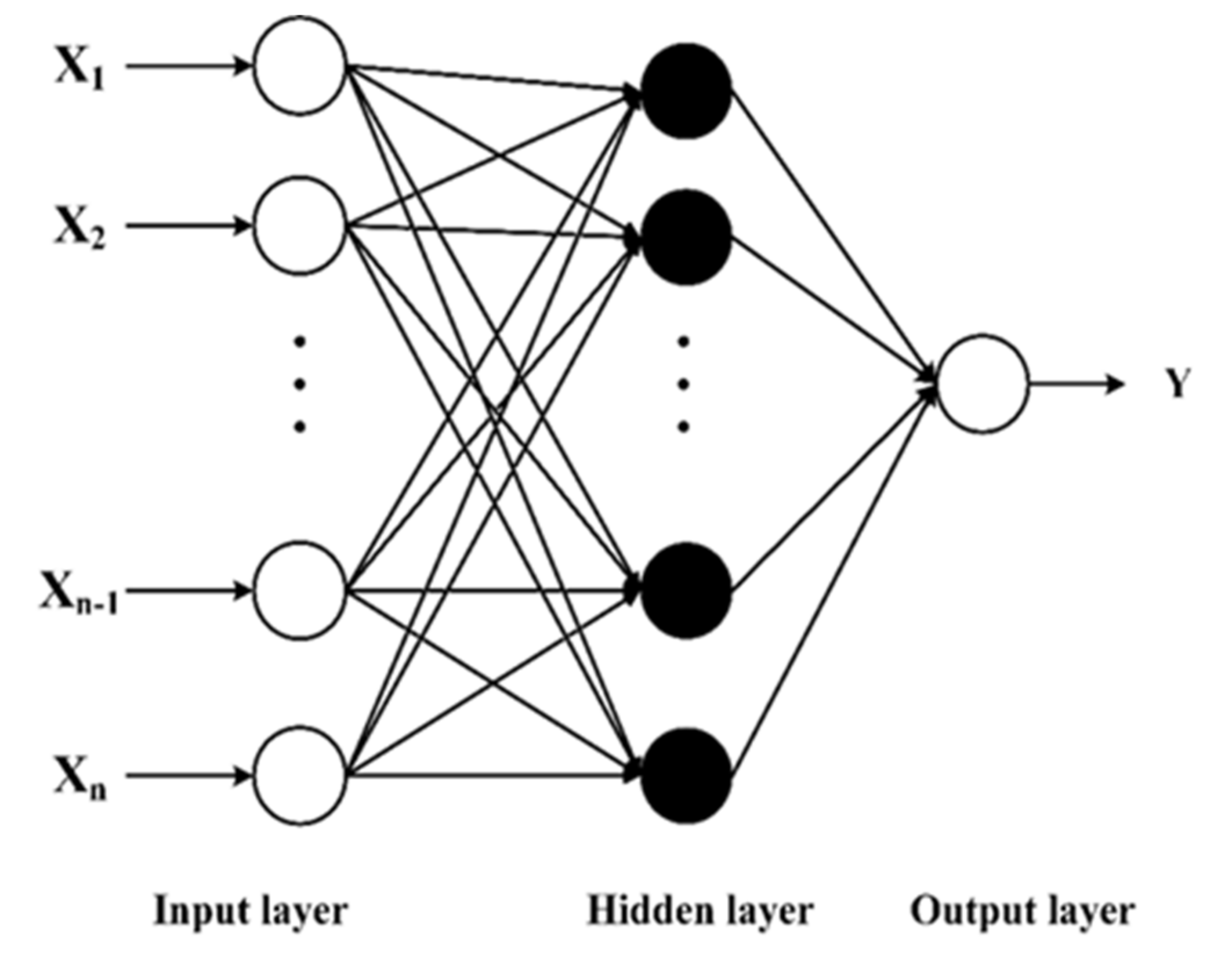
2.2. Feed-Forward Backpropagation Neural Network (FFBN)

The data collected for model construction are shown in Table 1. Because data were over 2 orders of magnitude, to overcome the influence of dimensions on the results, they were normalized into the interval of [−1,1] using Equation (1):

$${ \mathrm{X}}^{*}=\frac{2\mathrm{X}-{\mathrm{X}}_{\max -}{\mathrm{X}}_{\min }}{{\mathrm{X}}_{\max }-{\mathrm{X}}_{\min }}.$$

(1)

where X* is the normalized value, X is the observed value, X_max is the maximum value of X, X_min is the minimum value of X.

The tansig function was selected as the active function of neurons in the FFBN (Figure 2) (Equation (2)):

$$\mathrm{f}\left(\mathrm{x}\right)=\frac{2}{1+{\mathrm{e}}^{-2\mathrm{x}}}-1.$$

(2)

The number of neurons in the hidden layer, as proposed by Kolmogorov, is:

N = 2 m + 1

(3)

where N is the neuron number in the hidden layer, and m is the neuron number in the input layer.

However, it is difficult to determine a model’s optimal number of neurons based only on theory. To obtain the best neural network, the number of neurons of the network must be adjusted [21]. Based on modeling accuracy and generalization, we chose a network structure with similar prediction accuracy between the training and testing sets as the optimal architecture. Furthermore, the testing set with higher prediction accuracy was preferred [28].

2.3. Partial Least Squares Regression (PLSR)

Partial least square regression is a bilinear factor model, widely used in chemistry, economics, and pharmaceutical sciences. It has good performance when applied to a matrix X with many noisy and collinear factors. In this study, we used PLSR to predict the rice yield (matrix Y) using the climate and agronomic traits (matrix X).

The optimum factor number of the PLSR was determined by Equations (4)–(6):

$$S_{S\mathrm{S},h}={\displaystyle \sum }_{\mathrm{i}=1}^{\mathrm{n}}{\left({\mathrm{y}}_{\mathrm{i}}-{\widehat{y}}_{\mathrm{hi}}\right)}^2$$

(4)

$${\mathrm{S}}_{\mathrm{PRESS},\mathrm{h}}={\displaystyle \sum }_{\mathrm{i}=1}^{\mathrm{n}}{\left({\mathrm{y}}_{\mathrm{i}}-{\widehat{y}}_{\mathrm{h}\left(-\mathrm{i}\right)}\right)}^2$$

(5)

$${\mathrm{Q}}_{\mathrm{h}}{}^2=1-\frac{{\mathrm{S}}_{\mathrm{PRESS},\mathrm{h}}}{{\mathrm{S}}_{\mathrm{SS},\mathrm{h}}}$$

(6)

where $y_i$ is the raw data, ${\widehat{y}}_{hi}$ is the fitted value of the i-th sample point after using all sample points and taking the h component from regression modeling. ${\widehat{y}}_{h\left(-i\right)}$ represents deleting sample point i when modeling, taking the h component from regression modeling, and then using this model to calculate the fitted value of $y_i$. When ${\mathrm{Q}}_{\mathrm{h}}{}^2\ge 0.0975$, adding a new component significantly improves the predictive ability of the built model, otherwise the added new component has no significant meaning [29].

2.4. Model Evaluations

The relation coefficient (R²) and the root mean square error (RMSE) were used to evaluate the model performances.

$${ \mathrm{R}}^2=1-\frac{{{\displaystyle \sum }}_{\mathrm{i}=1}^{\mathrm{n}}{\left({\mathrm{y}}_{\mathrm{i}}-\widehat{{\mathrm{y}}_{\mathrm{i}}}\right)}^2}{{{\displaystyle \sum }}_{\mathrm{i}=1}^{\mathrm{n}}{\left({\mathrm{y}}_{\mathrm{i}}-\overline{{\mathrm{y}}_{\mathrm{i}}}\right)}^2}$$

(7)

$$\mathrm{RMSE}=\sqrt{\frac{{{\displaystyle \sum }}_{\mathrm{i}=1}^{\mathrm{n}}{\left({\mathrm{y}}_{\mathrm{i}}-\widehat{{\mathrm{y}}_{\mathrm{i}}}\right)}^2}{\mathrm{n}}}$$

(8)

where ${\mathrm{y}}_{\mathrm{i}}$ is the actual data, $\widehat{{\mathrm{y}}_{\mathrm{i}}}$ is the predicted data of the model, $\mathrm{n}$ is the number of samples.

MATLAB 2018a (MathWorks, Natick, MA, USA) was used for data analysis and model building.

3. Results and Discussion

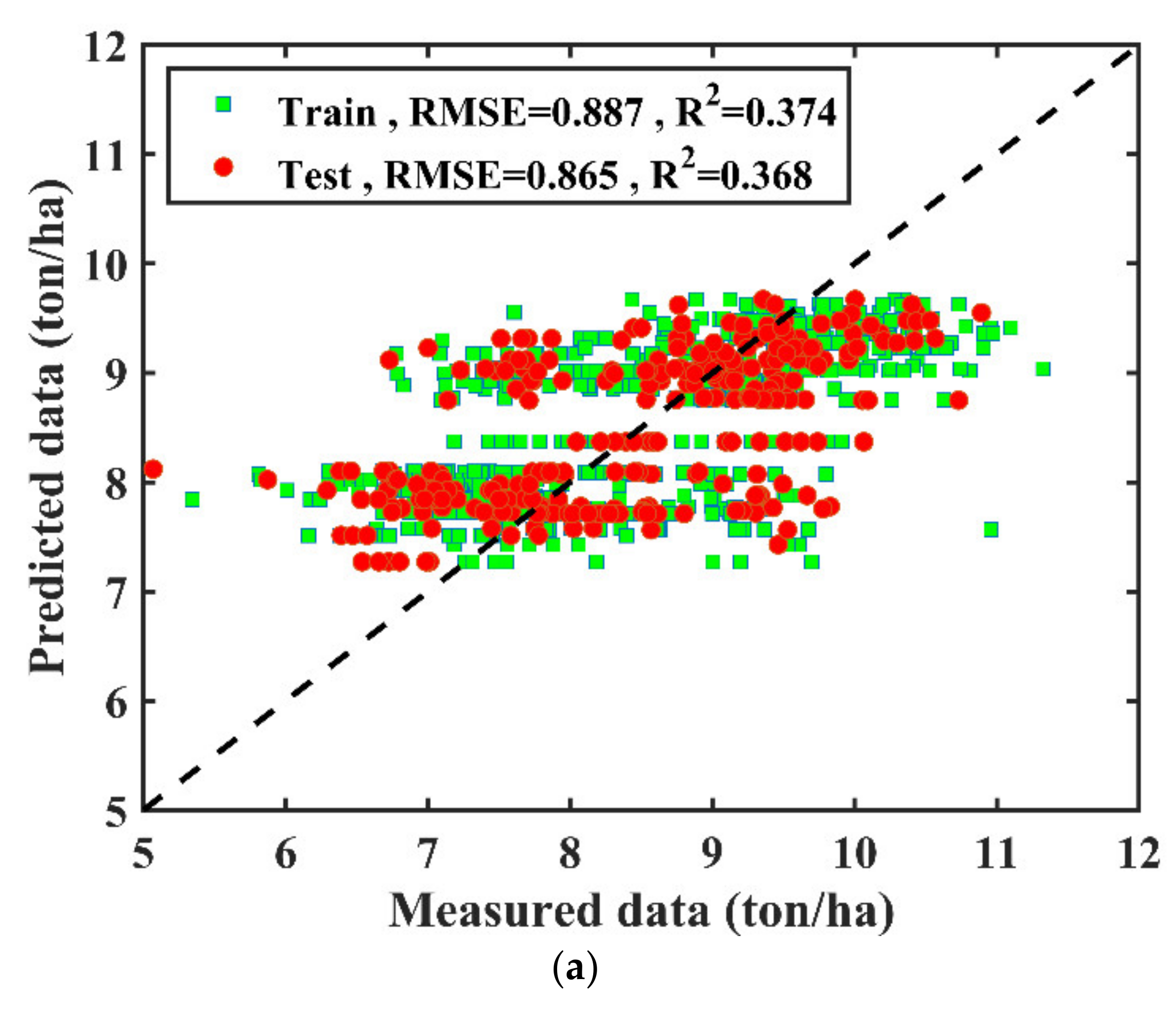
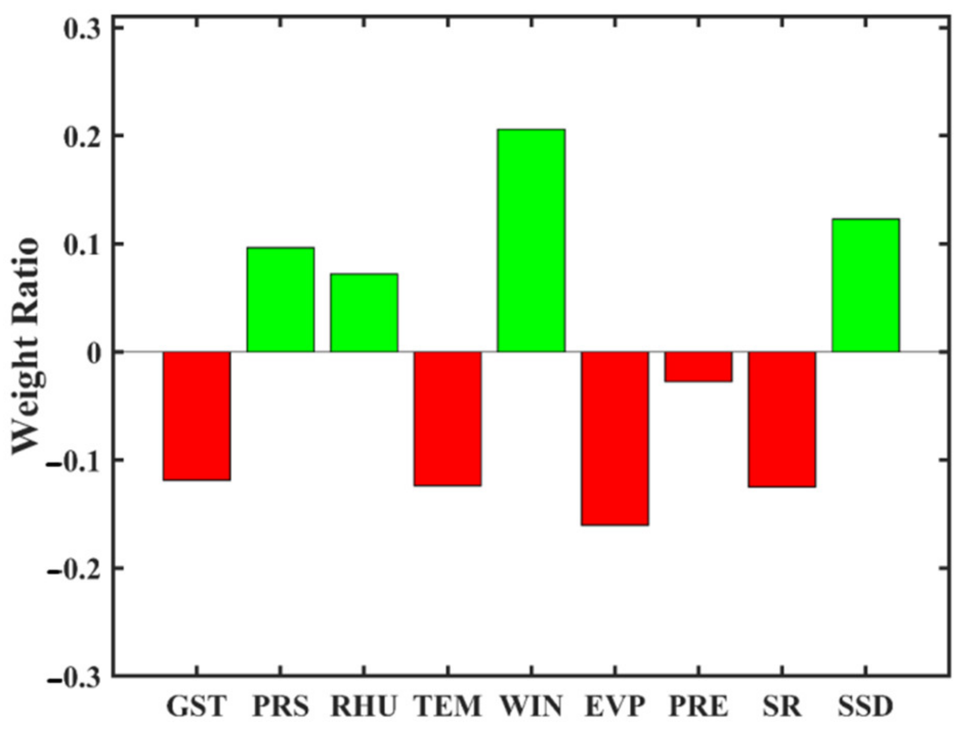
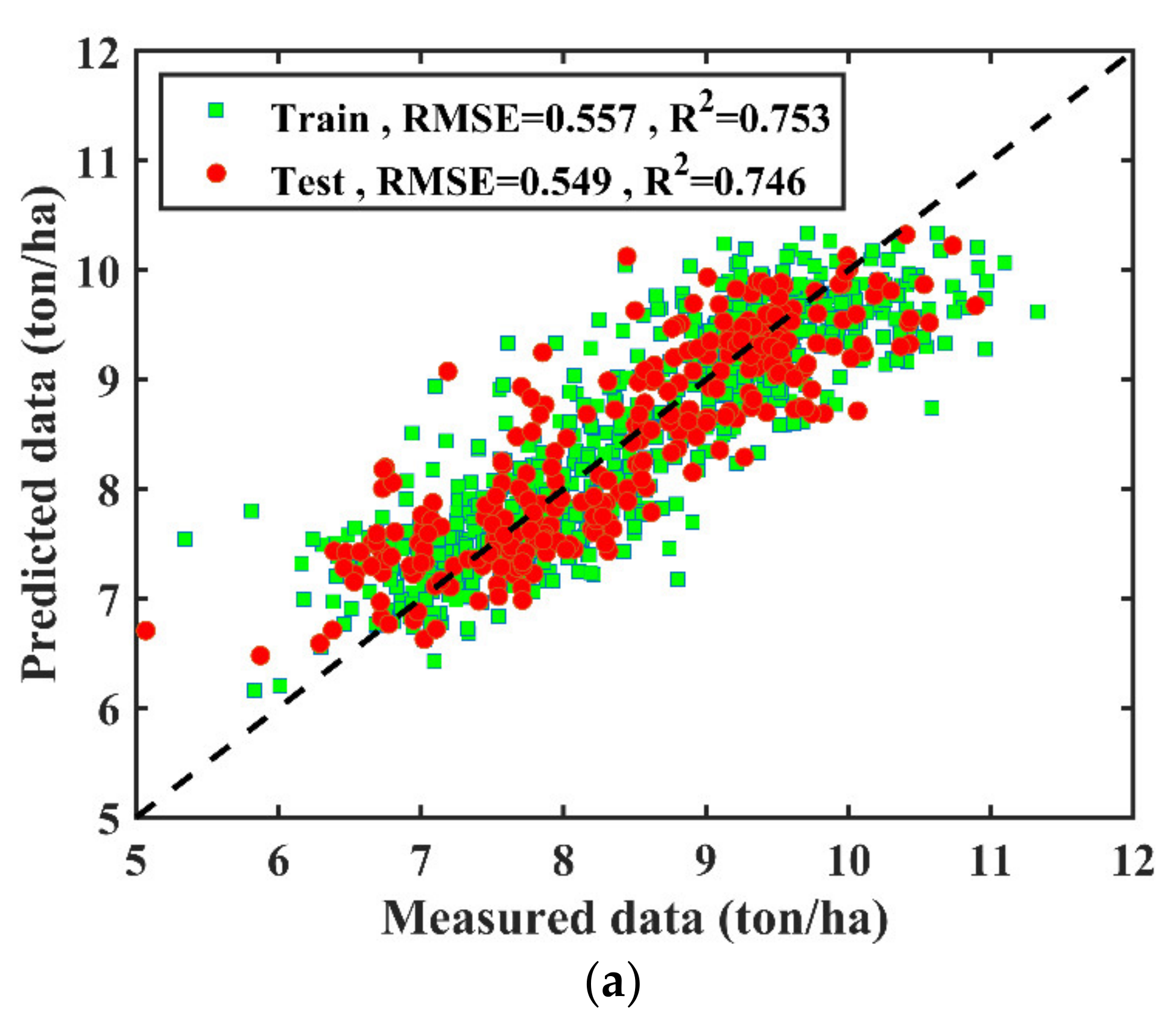
3.1. Climate Data Based Modeling

The scatter plots of the predicted values using PLSR and BPNN, and the observed data, are shown in Figure 3. In PLSR modeling, the R² was 0.374 for the training dataset and 0.368 for testing dataset, whereas the R² of the FFBN model was 0.611 and 0.578 for training and testing datasets, respectively. The RMSE of FFBN was therefore smaller than that of the PLSR model. Both models showed a significant relationship between measured and predicted values, indicating that the climate parameters contributed to the rice yield, and better prediction performance of FFBN was observed.

Rice yields have not only been predicted by linear models (multiple regression) in east Madhya [30] and at Kharagpur Lower Gangetic Plain in India [31,32,33], but also by nonlinear models (ANN and RF) [34,35]. PLSR and BPNN models were first applied in rice yield prediction; although similar R² values were obtained in these predictions, total prediction accuracy was improved in this study.

From PLSR modeling, it was found that GST, TEM, EVP, PRE, and SR showed negative correlation with rice yield, and the weight ratio of EVP was the largest; PRS, RHU, WIN, and SSR showed positive correlation with rice yield, and the weight ratio of WIN was the largest (Figure 4). This demonstrates that different climate parameters played significantly different roles in the prediction. Soil fertility should play a role in the modelling, but the qualification of soil properties was time-consuming and costly, which represents a challenge, particularly in areas with the same soil types. In addition, the roles might be changed for different regions, for example, rainfall could be the most important parameter in India [31].

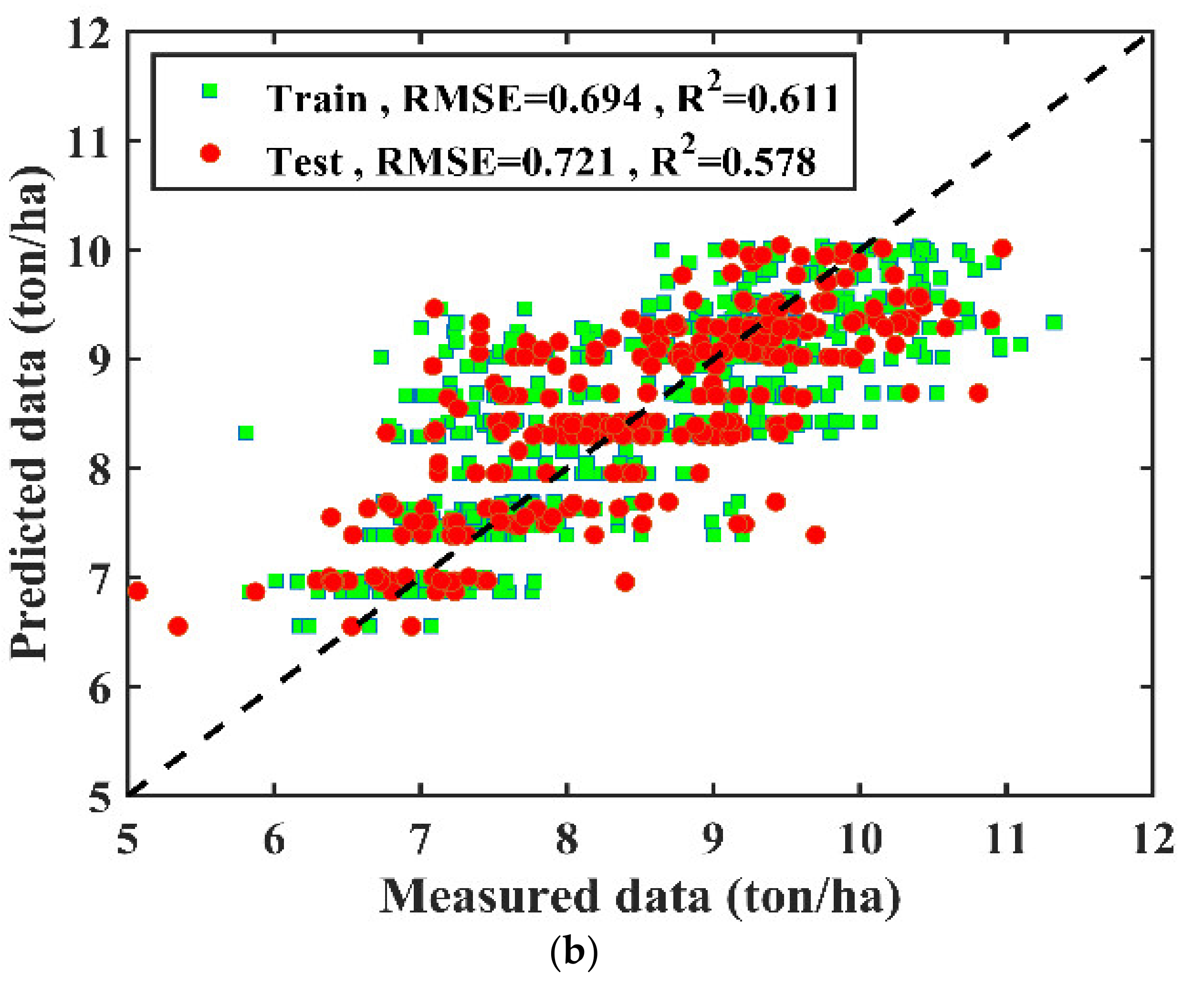
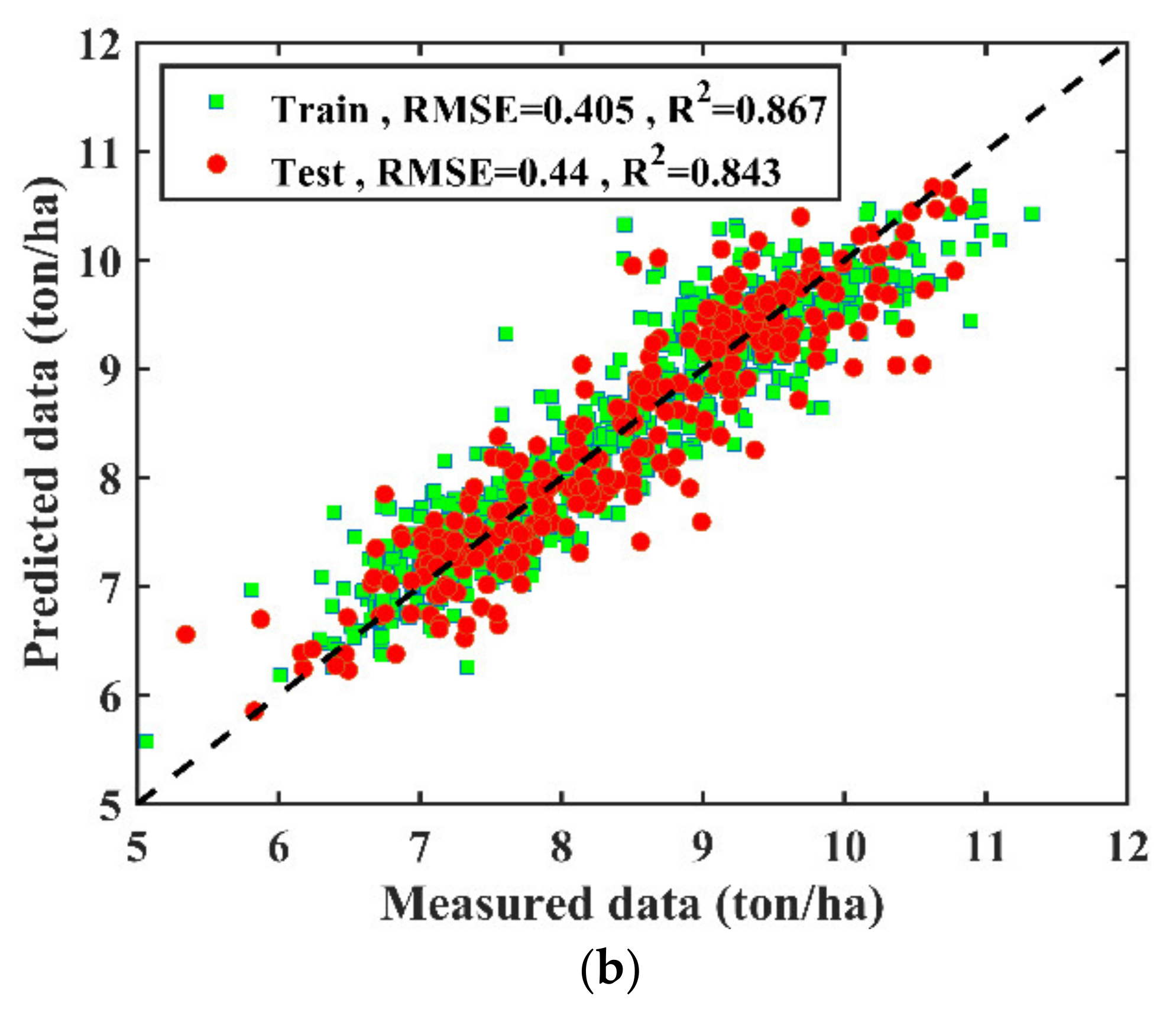
3.2. Agronomic Trait-Based Modeling

The scatter plots of the predictions of the PLSR and BPNN models, and the observed data, are demonstrated in Figure 5. In PLSR modeling, the R² was 0.707 for the training dataset and 0.689 for the testing dataset; the R² of the FFBN model was 0.750 and 0.742 for training and testing datasets, respectively; and the RMSE of PLSR and FFBN in the testing set was 0.608 and 0.556 ton/ha, respectively. Both models showed significant relationships between measured and predicted values. In addition, both models, particularly the PLSR model, were significantly improved using the agronomic trait data compared to using the climate data. This indicates a greater contribution was made by agronomic traits to the prediction, and better prediction performance of FFBN was also observed.

From PLSR modeling, it was found that all of the agronomic traits showed a positive correlation with rice yield, and the weight ratio of FGPP was the largest, whereas PH was the smallest (Figure 6).

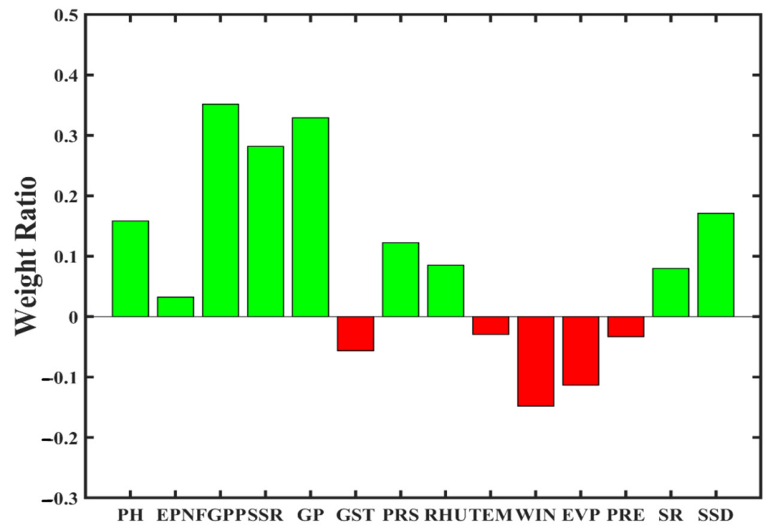
3.3. Climate and Agronomic Traits Data Fused Modelling

To improve the accuracy of the model, climate and agronomic trait data were fused to train the PLSR and FFBN model (Figure 7). In PLSR modeling, the R² was 0.753 for the training dataset and 0.746 for the testing dataset, and the R² of the FFBN model was 0.867 and 0.843 for the training and testing datasets, respectively; the RMSE of PLSR and FFBN in the testing set was 0.440 and 0.549 ton/ha, respectively. Both models, particularly the FFBN model, were significantly improved using the fused data. In addition, the FFBN model showed better prediction performance, which demonstrated that the nonlinear model performed better than the linear model in a complicated system.

Phenology and climate data have also been integrated into rice yield modeling using a variety of algorithms, including multiple linear regression, SVMs, and RFs [36]. The PLSR model in this study indicated a significantly improved performance compared to that of conventional multiple linear regression models, and the FFBN model also demonstrated significant improvements in R² and RMSE compared to those of other nonlinear ML models.

From data-fused PLSR modeling, it was found that the contributions of agronomic traits remained similar in the prediction, in which the largest change was that the weight ratio of EPN was found to be considerably smaller (Figure 8). However, it was found that significant changes occurred for the contributions of climate parameters. The contributions of PRS, RHU, and SSD remained positive, and GST, TEM, EVP, and PRE remained negative, whereas the contributions of WIN and SR reversed. Notably, WIN reversed from the most positive into the most negative parameter, which indicates significant interactions occurred among climate parameters and agronomic traits. Therefore, the covariates from climate parameters and agronomic traits functioned in the prediction. Although climate parameters can be used to directly predict rice yield, impacts should be considered regarding the covariates, and modifications should be considered in applications.

4. Conclusions

The rice yield was well predicted by nonlinear FFBN and linear PLSR models using climate data and agronomic trait data. The agronomic trait data indicated larger contributions to the predictions than the climate data, and data fusion further improved the prediction capability of the models. The FFBN model showed better prediction performance using the optimum neural network architecture of one hidden layer with 29 neurons. The climate factors of wind speed and evaporation, and the agronomic traits of filled grains per panicle and growth period, made significant contributions to the predictions. Covariates occurred among agronomic traits and climate parameters, and the contributions of climate parameters were significantly impacted by the covariates. Although climate data could be used for rice prediction, proper modifications should be made to improve the reliability and accuracy of the modelling.

References

1. FAO. Global Climate Changes and Rice Food Security; FAO: Rome, Italy, 2004. [Google Scholar]
2. Center, A.R. CGIAR Research Program 3.3: GRiSP-A Global Rice Science Partnership. 2010. Available online: https://cgspace.cgiar.org/handle/10947/5312 (accessed on 3 February 2021).
3. Cheng, S.H.; Zhuang, J.Y.; Fan, Y.Y.; Du, J.H.; Cao, L.Y. Progress in research and development on hybrid rice: A super-domesticate in China. Ann. Bot. 2007, 100, 959–966. [Google Scholar] [CrossRef]
4. Son, N.-T.; Chen, C.F.; Chen, C.R.; Guo, H.Y.; Cheng, Y.S.; Chen, S.L.; Lin, H.S.; Chen, S.H. Machine learning approaches for rice crop yield predictions using time-series satellite data in Taiwan. Int. J. Remote Sens. 2020, 41, 7868–7888. [Google Scholar] [CrossRef]
5. Hossain, M.A.; Uddin, M.N.; Hossain, M.A.; Jang, Y.M. Predicting rice yield for Bangladesh by exploiting weather conditions. In Proceedings of the 2017 International Conference on Information and Communication Technology Convergence (ICTC), Jeju Island, Korea, 18–20 October 2017; pp. 589–594. [Google Scholar]
6. Abdipour, M.; Younessi-Hmazekhanlu, M.; Ramazani, S.H.R. Artificial neural networks and multiple linear regression as potential methods for modeling seed yield of safflower (Carthamus tinctorius L.). Ind. Crops Prod. 2019, 127, 185–194. [Google Scholar] [CrossRef]
7. Emamgholizadeh, S.; Parsaeian, M.; Baradaran, M. Seed yield prediction of sesame using artificial neural network. Eur. J. Agron. 2015, 68, 89–96. [Google Scholar] [CrossRef]
8. Pantazi, X.E.; Moshou, D.; Alexandridis, T.; Whetton, R.L.; Mouazen, A.M. Wheat yield prediction using machine learning and advanced sensing techniques. Comput. Electron. Agric. 2016, 121, 57–65. [Google Scholar] [CrossRef]
9. Park, S.J.; Hwang, C.S.; Vlek, P.L.G. Comparison of adaptive techniques to predict crop yield response under varying soil and land management conditions. Agric. Syst. 2005, 85, 59–81. [Google Scholar] [CrossRef]
10. Dabrowska-Zielinska, K.; Kogan, F.; Ciolkosz, A.; Gruszczynska, M.; Kowalik, W. Modelling of crop growth conditions and crop yield in Poland using AVHRR-based indices. Int. J. Remote Sens. 2002, 23, 1109–1123. [Google Scholar] [CrossRef]
11. Fang, H.; Liang, S.; Hoogenboom, G.; Teasdale, J.; Cavigelli, M. Corn-yield estimation through assimilation of remotely sensed data into the CSM-CERES-Maize model. Int. J. Remote Sens. 2008, 29, 3011–3032. [Google Scholar] [CrossRef]
12. Bala, S.K.; Islam, A.S. Correlation between potato yield and MODIS-derived vegetation indices. Int. J. Remote Sens. 2009, 30, 2491–2507. [Google Scholar] [CrossRef]
13. Mkhabela, M.S.; Bullock, P.; Raj, S.; Wang, S.; Yang, Y. Crop yield forecasting on the Canadian Prairies using MODIS NDVI data. Agric. For. Meteorol. 2011, 151, 385–393. [Google Scholar] [CrossRef]
14. Son, N.T.; Chen, C.F.; Chen, C.R.; Minh, V.Q.; Trung, N.H. A comparative analysis of multitemporal MODIS EVI and NDVI data for large-scale rice yield estimation. Agric. For. Meteorol. 2014, 197, 52–64. [Google Scholar] [CrossRef]
15. Boser, B.E.; Guyon, I.M.; Vapnik, V.N. A training algorithm for optimal margin classifiers. In Proceedings of the Fifth Annual Workshop on Computational Learning Theory, Pittsburgh, PA, USA, 27–29 July 1992; pp. 144–152. [Google Scholar]
16. Breiman, L. Random forests. Mach. Learn. 2001, 45, 5–32. [Google Scholar] [CrossRef] [Green Version]
17. Liakos, K.G.; Busato, P.; Moshou, D.; Pearson, S.; Bochtis, D. Machine learning in agriculture: A review. Sensors 2018, 18, 2674. [Google Scholar] [CrossRef] [Green Version]
18. Mountrakis, G.; Im, J.; Ogole, C. Support vector machines in remote sensing: A review. ISPRS J. Photogramm. Remote Sens. 2011, 66, 247–259. [Google Scholar] [CrossRef]
19. Du, C.; Tang, D.; Zhou, J.; Wang, H.; Shaviv, A. Prediction of nitrate release from polymer-coated fertilizers using an artificial neural network model. Biosyst. Eng. 2008, 99, 478–486. [Google Scholar] [CrossRef]
20. Kung, H.-Y.; Kuo, T.-H.; Chen, C.-H.; Tsai, P.-Y. Accuracy analysis mechanism for agriculture data using the ensemble neural network method. Sustainability 2016, 8, 735. [Google Scholar] [CrossRef] [Green Version]
21. Li, W.; Wei, S.; Jiao, W.; Qi, G.; Liu, Y. Modelling of adsorption in rotating packed bed using artificial neural networks (ANN). Chem. Eng. Res. Des. 2016, 114, 89–95. [Google Scholar] [CrossRef]
22. Liu, Z.-W.; Liang, F.-N.; Liu, Y.-Z. Artificial neural network modeling of biosorption process using agricultural wastes in a rotating packed bed. Appl. Therm. Eng. 2018, 140, 95–101. [Google Scholar] [CrossRef]
23. Pham, B.T.; Nguyen, M.D.; Bui, K.-T.T.; Prakash, I.; Chapi, K.; Bui, D.T. A novel artificial intelligence approach based on Multi-layer Perceptron Neural Network and Biogeography-based Optimization for predicting coefficient of consolidation of soil. Catena 2019, 173, 302–311. [Google Scholar] [CrossRef]
24. Zhao, B.; Su, Y.; Tao, W. Mass transfer performance of CO2 capture in rotating packed bed: Dimensionless modeling and intelligent prediction. Appl. Energy 2014, 136, 132–142. [Google Scholar] [CrossRef]
25. De Freitas, E.C.S.; de Paiva, H.N.; Neves, J.C.L.; Marcatti, G.E.; Leite, H.G. Modeling of eucalyptus productivity with artificial neural networks. Ind. Crops Prod. 2020, 146. [Google Scholar] [CrossRef]
26. Gilardelli, C.; Stella, T.; Frasso, N.; Cappelli, G.; Bregaglio, S.; Chiodini, M.E.; Scaglia, B.; Confalonieri, R. WOFOST-GTC: A new model for the simulation of winter rapeseed production and oil quality. Field Crops Res. 2016, 197, 125–132. [Google Scholar] [CrossRef]
27. Niazian, M.; Sadat-Noori, S.A.; Abdipour, M. Modeling the seed yield of Ajowan (Trachyspermum ammi L.) using artificial neural network and multiple linear regression models. Ind. Crops Prod. 2018, 117, 224–234. [Google Scholar] [CrossRef]
28. Meshram, S.G.; Singh, V.P.; Kisi, O.; Karimi, V.; Meshram, C. Application of artificial neural networks, support vector machine and multiple model-ann to sediment yield prediction. Water Resour. Manag. 2020, 34, 4561–4575. [Google Scholar] [CrossRef]
29. Abdi, H. Partial least squares regression and projection on latent structure regression (PLS Regression). Wiley Interdiscip. Rev. Comput. Stat. 2010, 2, 97–106. [Google Scholar] [CrossRef]
30. Giri, A.K.; Bhan, M.; Agrawal, K.K. Districtwise wheat and rice yield predictions using meteorological variables in eastern Madhya Pradesh. J. Agrometeorol. 2017, 19, 366–368. [Google Scholar]
31. Dhekale, B.S.; Nageswararao, M.M.; Nair, A.; Mohanty, U.C.; Swain, D.K.; Singh, K.K.; Arunbabu, T. Prediction of kharif rice yield at Kharagpur using disaggregated extended range rainfall forecasts. Theor. Appl. Climatol. 2018, 133, 1075–1091. [Google Scholar] [CrossRef]
32. Rakhee; Singh, A.; Kumar, A. Weather based fuzzy regression models for prediction of rice yield. J. Agrometeorol. 2018, 20, 297–301. [Google Scholar]
33. Biswas, R.; Bhattacharyya, B. Rice yield prediction in lower Gangetic Plain of India through multivariate approach and multiple regression analysis. J. Agrometeorol. 2019, 21, 101–103. [Google Scholar]
34. Das, B.; Nair, B.; Reddy, V.; Venkatesh, P. Evaluation of multiple linear, neural network and penalised regression models for prediction of rice yield based on weather parameters for west coast of India. Int. J. Biometeorol. 2018, 62, 1809–1822. [Google Scholar] [CrossRef]
35. Kim, J.; Lee, J.; Sang, W.G.; Shin, P.; Cho, H.; Seo, M.C. Rice yield prediction in South Korea by using random forest. Korean J. Agric. For. Meteorol. 2019, 21, 75–84. [Google Scholar]
36. Guo, Y.; Fu, Y.; Hao, F.; Zhang, X.; Wu, W.; Jin, X.; Robin Bryant, C.; Senthilnath, J. Integrated phenology and climate in rice yields prediction using machine learning methods. Ecol. Indic. 2021, 120. [Google Scholar] [CrossRef]
Figure 1. Location of the study area and climate stations in China.
Agronomy 11 00282 g001
Figure 2. The basic structure of applied neural networks.
Agronomy 11 00282 g002
Figure 3. (a) Performance of partial least squares regression (PLSR) model with optimized PLS factor of 2 for training and testing sets using climate data; (b) performance of feed-forward backpropagation neural network (FFBN) model with optimized number of neurons of 13 in the hidden layer for training and testing sets using climate data.
Agronomy 11 00282 g003aAgronomy 11 00282 g003b
Figure 4. Weight ratio of climate parameters from the PLSR model for training and testing sets using climate data. GST, ground surface temperature (°C); PRS, pressure of the station (hPa); RHU, relative humidity (%); TEM, temperature (°C); WIN, wind speed (m/s); EVP, evaporation (mm); PRE, precipitation (mm); SR, solar radiation (MJ/m2); SSD, sunshine duration (hour); YIELD, rice yield (ton/ha).
Agronomy 11 00282 g004
Figure 5. (a) Performance of PLSR model with optimized PLS factor of 4 for training and testing sets using agronomic traits data; (b) Performance of FFBN model with optimized neurons of 10 in hidden layer for train and test set using agronomic traits data.
Agronomy 11 00282 g005
Figure 6. Weight ratio from PLSR model for training and testing sets using agronomic trait data. PH, plant height (cm); EPN, effective panicle number (ten thousands/hm2); FGPP, filled grains per panicle (grains); SSR, seed set rate (%); GP, growth period (day).
Agronomy 11 00282 g006
Figure 7. (a) Performance of the PLSR model with optimized PLS factor of 4 for training and testing sets using fused data; (b) performance of the FFBN model with optimized number of neurons of 29 in the hidden layer for training and testing sets using fused data.
Agronomy 11 00282 g007aAgronomy 11 00282 g007b
Figure 8. Weight ratio from the PLSR model for training and testing sets using fused climate data and agronomic trait data. GST, ground surface temperature (°C); PRS, pressure of the station (hPa); RHU, relative humidity (%); TEM, temperature (°C); WIN, wind speed (m/s); EVP, evaporation (mm); PRE, precipitation (mm); SR, solar radiation (MJ/m2); SSD, sunshine duration (hour); YIELD, rice yield (ton/ha); PH, plant height (cm); EPN, effective panicle number (ten thousands/hm2); FGPP, filled grains per panicle (grains); SSR, seed set rate (%); GP, growth period (day).
Agronomy 11 00282 g008