Emulators of a Physical Model for Estimating Leaf Wetness Duration

Abstract

Leaf wetness duration (LWD) has rarely been measured due to lack of standard protocol. Thus, empirical and physical models have been proposed to resolve this gap. Although the physical model provides robust performance in diverse conditions, it requires many variables. The empirical model requires fewer variables; nevertheless, its performance is specific to a given condition. A universal LWD estimation model using fewer variables is thus needed to improve LWD estimation. The objective of this study was to develop emulators of the LWD estimation physical model for use as universal empirical models. It is assumed that the Penman–Monteith (PM) model determines LWD and can be employed as a physical model. In this study, a simulation was designed and conducted to investigate the characteristics of the PM model and to build the emulators. The performances of the built emulators were evaluated based on a case study of LWD data obtained in South Korea. It was determined that a machine learning algorithm can properly emulate the PM model in LWD estimations based on the simulation. Moreover, the poor performances of some emulators that use wind speed may have been due to the limitation of wind speed measurement. The accuracy of the anemometer is thus critical to estimating LWD using physical models. A deep neural network using relative humidity and air temperature was found to be the most appropriate emulator of those tested for LWD estimation.

1. Introduction

Leaf wetness (LW) and leaf wetness duration (LWD) are important parameters in plant disease epidemiology [1]. LWD is the extent of time in which free water exists on the surface of plant tissue. Many studies have reported that LW and plant diseases resulting from bacteria and fungi are strongly correlated in temperatures that are favorable to infection [2,3]. This relation has been widely used to predict the development of plant diseases and to support decision making in agriculture management [4,5,6].

As LWD is a non-standard meteorological variable approved by the World Meteorological Organization (WMO), it is not widely measured. Hence, several methods have been proposed to estimate LWD using the standard meteorological variables. Moreover, many physical and empirical models have been suggested to estimate LWD using these variables [7,8,9,10,11]. Physical and empirical models have respective positive and negative aspects. The physical models have the advantage of being applied in diverse geographical areas and environmental conditions. When the many input variables that are required in the physical model are available, the physical models can accurately estimate LWD. However, these input variables, which include cloud cover, albedo, and net radiation, are frequently inaccessible. Additionally, the results of these models are very sensitive to input variable changes [12].

Some empirical models, e.g., the relative humidity (RH)-threshold-based model, dew point depression model, classification and regression tree model, and neural network model, have been proposed to overcome the limitations of the physical models [13,14,15,16]. The empirical model inherently fits the dataset used in developing that model. Thus, to estimate LWD in other regions, the model should be calibrated by using a dataset obtained from the region of interest. Hence, the empirical model provides a limited LWD estimation when the observed LWD data are unavailable owing to a lack of calibration.

If the meteorological and LW data that represent various environmental conditions are available, the empirical model provides robust performance under different environmental conditions. This model can be developed by using such datasets. In reality, however, these datasets are difficult to obtain on account of several factors, such as a lack of standard protocols for measuring LW as well as insufficient availability of LW and LWD data. Nonetheless, LW data can be generated by the physical models using meteorological data. If the meteorological data can represent the characteristics of the diverse environmental conditions, the generated LW data can have similar characteristics. The empirical model developed by the generated LW and meteorological data may provide consistent performance for estimating LW and LWD in many regions in the world. Furthermore, the efficiency of the empirical model may be high since the required input data in the empirical model can be customized by users. Hence, the empirical model can improve the accessibility of LWD data in regions where the data are scarce. The empirical model based on the generated data is considered an emulator of the physical model because the data are generated by the physical model.

In this paper, emulators of the physical model for LWD estimation are proposed as universal empirical models. The Penman–Monteith (PM) model is employed as the physical model for LWD estimation. The possible ranges of the input variables in the PM model for cultivating vegetation are investigated. Combinations of the input variables are selected based on these possible ranges, and the LW data are generated through their combination. LW estimation is a binary classification problem. Several machine learning (ML) algorithms are employed for modeling the relation between the input variable and LW. A simulation study is designed and conducted to investigate the PM model characteristics and to build the emulators. The performances of the built emulators are evaluated based on a case study of LWD data obtained in South Korea. The emulators built in this study will enhance our ability to estimate LW and LWD. Particularly, the emulators may be a good alternative to estimating LWD in regions with scarce data. In addition, the simulation results will improve our application of the PM model for LWD estimation.

The remainder of this paper is organized as follows. In Section 2, the theoretical background of this study, including the PM model, ML algorithms, and evaluation measures, is described. The design and results of the simulation for developing emulators using generated data are presented in Section 3. As the emulators are developed based on generated data, the performances of emulators should be evaluated based on real-world data. In Section 4, the case study for assessing the performances of emulators based on real-world data and its results are described. Finally, in Section 5, the discussion and conclusions are presented.

2. Theoretical Background

2.1. Penman–Monteith Model for LW Estimation

The PM model predicts the occurrence of wetness on a leaf surface based on latent heat flux (LE), which can indicate moisture condensation in air on a free surface [17]. This model can predict LW in any place where the required meteorological observations are accessible because it is based on the physical mechanism of the LW occurrence. Sentelhas et al. [18] showed that the PM model provides good performance and has high applicability owing to low spatial variation in different environments. In addition, data on the air temperature at the leaf level are not required to predict LW. Moreover, any vegetation type can be applicable in the PM model, unlike other LW estimation models based on a physical mechanism. This factor is also a limitation of the PM model that requires additional modification for vegetation characteristics. The PM model can predict LW on a mock leaf for each interval of time [19]. Therefore, the PM model was employed as a universal LWD estimation model in the current study. The equation of LE in the PM model is given in Equation (1).

$$\mathrm{LE}=-\frac{s{R}_n+\left[1200\left(e_s-e_a\right)/\left(r_a+r_b\right)\right]}{s+\gamma }$$

(1)

where s, $R_n$, $e_s$, $e_a$, $\gamma$, $r_b$, and $r_a$ are the slope of the saturation vapor pressure curve (hPa), net radiation of the mock leaf (W/m²), saturated vapor pressure at the weather station air temperature (hPa), actual air vapor pressure (hPa), modified psychrometer constant (0.64 kPa/K is adopted here), boundary layer resistance for heat transfer, and boundary layer resistance for wind speed (WS, m/s), respectively. $R_n$ can be calculated by Equation (2) [20,21].

$$R_n=\frac{\left(ns-nl\right)}{24}$$

(2)

$$ns=100\left(1-ab\right)\mathrm{SW}$$

(3)

$$nl=\left(4.901\mathrm{e}-07\right)\frac{R_s}{R_{so}} \left(0.34-0.14{\left(\frac{e_a}{10}\right)}^{0.5}\right){\left(T+237.3\right)}^4$$

(4)

where ns, nl, SW, T, ab, and $\frac{R_s}{R_{so}}$ are the net short-wave radiation (W/m²), net long-wave radiation (W/m²), short-wave radiation (W/m²), air temperature (°C), albedo (or canopy reflection), and relative short-wave radiation (RSR), which is the ratio of solar radiation ($R_s$) to clean-sky solar radiation ($R_{so}$) and is limited to being ≤1, respectively. Moreover, $e_s$, $e_a$, and s are given by Equations (5)–(7), respectively [20].

$$e_s=6.108\exp \left(\frac{17.27T}{T+237.2}\right)$$

(5)

$$e_a=6.108\exp \left(\frac{17.27T_d}{T_d+237.2}\right)$$

(6)

$$s=\frac{4098\left(0.6108\exp \left(\frac{17.27T}{T+237.2}\right)\right)}{{\left(T+237.3\right)}^2}$$

(7)

where $T_d$ is the dew point temperature (°C). $T_d$ is converted using the relative humidity (RH) by Equation (8) [20].

$$T_d={\left(\frac{\mathrm{RH}}{100}\right)}^{0.125}\left(112+0.9T\right)+0.1T-112$$

(8)

here, ${\mathrm{r}}_{\mathrm{b}}$ can be calculated by Equation (9).

$${\mathrm{r}}_{\mathrm{b}}=307{\left(\frac{\mathrm{D}}{\mathrm{WS}}\right)}^{0.5}$$

(9)

where D is the effective dimension of the mock leaf (m). ${\mathrm{r}}_{\mathrm{a}}$ is given by Equation (10).

$${\mathrm{r}}_{\mathrm{a}}=\frac{\ln \left[\left(Z_s-d\right)/\left(Z_0\right)\right]}{0.4{\mathrm{WS}}^{*}}$$

(10)

where $Z_s$, d, $Z_0$, and ${\mathrm{WS}}^{*}$ are the height of the wetness sensor (m), displacement height (0.5 Z_c), roughness length (0.13 Z_c), and friction velocity (m/s), respectively. Z_c is the crop height. For LE estimates at the weather station, where the wetness sensor is at the same level as the T, RH and WS sensors, the boundary layer resistance for WS is not required in Equation (1). In the current study, Equation (1) is used to predict LE since the levels of T, RH and WS sensors are different. When LE is greater than zero, LW is predicted at the specific time.

2.2. Candidate ML Algorithms of the PM Emulator for LW Prediction

The ML algorithm can be a good alternative for emulating the PM model for LW estimation. It is a binary classification problem because the ML algorithm has been broadly employed as the solution to the classification problem [22,23,24]. In the current study, the extreme learning machine (ELM), random forest (RF), support vector machine (SVM), and deep neural network (DNN) were tested for use in the candidate algorithms of the PM emulator. Since these models showed good performance in estimating LW and LWD in other studies [14,25,26], they were expected to produce good performances for emulating the PM model. Brief descriptions of these algorithms are presented in the following subsections.

2.2.1. Extreme Learning Machine

ELM is a single-layer feed-forward network with input weights and biases that are randomly created [27]. Unlike traditional neural networks, the ELM can be trained in a single iteration owing to adoption of the randomized input weight and bias. It can be expressed by the following equation:

$$Y=\mathbf{H}\mathsf{\beta }$$

(11)

where Y, β, and H are the labels, the weight matrix between the hidden layer and the output layer, and the output vector of the hidden layer, respectively. It is called nonlinear feature mapping.

$$H={\mathrm{f}}_{\mathrm{a}}\left(XW+B\right)$$

(12)

where ${\mathrm{f}}_{\mathrm{a}}\left(·\right)$, W, B, and X are the activation function, input weight matrix, hidden layer bias, and input feature, respectively. The sigmoid function (${\mathrm{f}}_{\mathrm{a}}\left(\mathrm{x}\right)=\frac{1}{1+\exp (-x)}$) is used as the activation function in the ELM. As the weights (W) and bias (B) are randomly generated, and the activation function (${\mathrm{f}}_{\mathrm{a}}\left(·\right)$) is known in the ELM, H is a deterministic variable from the dataset. Hence, only β needs to be found in the ELM.

In the ELM, finding the appropriate output weight set is an important task, as it is in a traditional artificial neural network. Finding the weights in the ELM can be considered as fitting a linear regression model using ordinary least squares. Ridge regression is employed to attenuate the multi-collinearity in the dataset by adding a norm of parameters in the parameter estimation of the regression model [28]. The ELM model also adopts this methodology in finding the output weights. The ELM attempts to achieve better generalization performance by reaching not only the smallest training error but also the smallest norm of output weights. This minimization problem can take the form of ridge regression or regularized least squares as follows [29]:

$$\min \frac{1}{2}\Vert \mathsf{\beta }{\Vert }^2+\frac{C}{2}\Vert \mathbf{H}\mathsf{\beta }-Y{\Vert }^2$$

(13)

where the first term of the objective function is an l₂ norm regularization term that controls the complexity of the model. The second term indicates the training error associated with the learned model. C > 0 is a tuning parameter. The ELM gradient equation can be analytically solved, and the closed-form solution can be written as the following:

$$\widehat{\mathsf{\beta }}={\left(H^{T}H+\frac{1}{C}I\right)}^{-1}{H}^{T}Y$$

(14)

where I is an identity matrix.

2.2.2. Random Forest

RF has been frequently employed as a classifier in classification problems [30,31]. RF was proposed by Breiman [32] and uses bagging to build a number of decision trees. Thus, the RF consists of several simple decision trees. Each decision tree in the RF is grown using randomly selected samples. Subsequently, the nodes in each tree use randomly selected input features. The RF has two major characteristics: (1) randomness and (2) ensemble learning.

Random sampling of the entire dataset and the random selection of features led to RF randomness in this study. Every decision tree that was a simple classifier was built with randomness. The features in the dataset were randomly sampled and replaced to create a subset that was used to train one decision tree. At each node, the optimal split rule was determined using the randomly selected feature from the candidate features. Approximately two-thirds of the data were selected as the training subset. The features were also randomly selected without being replaced. The dataset that was not included in the training subset was deemed out-of-bag, and it assessed the appropriateness of the decision trees and the importance of the features.

The ensemble learning method in the RF means that all individual decision trees in the collection of decision trees (called an ensemble) contribute to the final prediction. A training subset is created after the random selection step. The classification and regression tree, although not pruned, was used in this study to construct a single decision tree. To grow K number of trees in the ensemble, this process (resampling a subset and training an individual tree) was repeated K times. The final predicted label was the most frequent label among the predicted labels of all individual trees. The “Ranger” library in the R package was used to construct the RF model [33].

2.2.3. Support Vector Machine

SVM is applied as a classifier for several classification problems in various fields [34]. SVM was developed for solving classification problems based on mathematics, unlike other machine learning algorithms, such as ELM, RF, and the gradient boosting machine (GBM). For example, for linear classification problems, every procedure in the SVM can be proved on a mathematical basis. SVM was developed for building classifiers that maximize the margin, that is, the distance between any two groups. The distance between two groups is determined by the distance between the support vectors, that is, the nearest vector to another group. In the current study, ν-SVM was employed for the SVM algorithm [35]. To find the hyperplane for maximizing the margin between the support vectors, the following optimization problem with its constraints had to be solved.

$$\min \tau \left(W,\xi ,\rho \right)=\frac{1}{2}\Vert W{\Vert }^2-\nu \rho +\frac{1}{2}{{\displaystyle \sum }}_{i=1}^n{\xi }_i$$

(15)

$$\mathrm{subject} \mathrm{to} y_i\left(\mathbf{\Theta }\left(X_i\right)W+b\right)\ge \rho -{\xi }_i,i=1,\dots ,n$$

(16)

$${\xi }_i\ge 0, \rho \ge 0$$

(17)

where $\nu$, ${\xi }_i$, and $\mathbf{\Theta }\left(·\right)$ are the respective regularization constant ranging from 0 to 1, the slack variable for the ith data point, and the kernel function that is the radial basis function ($\Theta \left(x_i,x_j\right)=\exp \left(-\frac{\Vert x_i-x_j{\Vert }^2}{2l^2}\right)$). The ν-SVM for the LW prediction model was implemented using the “e1071” library in R.

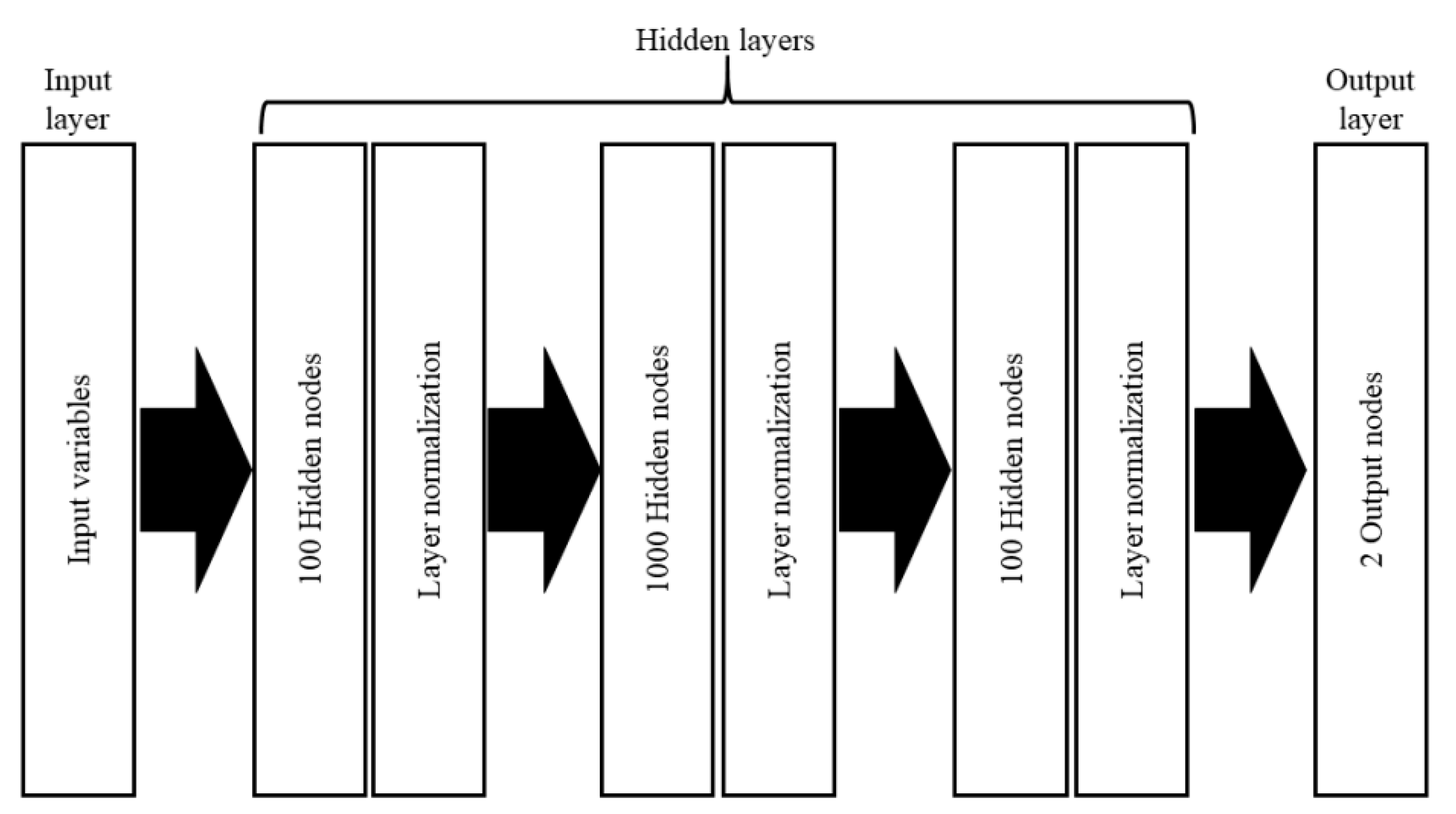
2.2.4. Deep Neural Network

DNN is a multiple-hidden layer feed-forward network. The main difference between a shallow neural network (ELM in this study) and DNNs is the number of hidden layers in the network. The deep hidden layer of the DNN allows for the emulation of a complex function relation between the input and output with the extraction of the complicated feature structure. In this study, the sigmoid function was used for the activation function of the DNN model. Four hidden layers were adopted for the employed DNN model, and each of these hidden layers had a different number of nodes. The structure of the DNN model was manually optimized. Although there are many methods for optimizing hyperparameters [36,37], they are not employed in the current study due to the limited computation resources. In addition, layer normalization was adopted after the second, third, and fourth hidden layers. Layer normalization improves the accuracy of the trained DNN model [38]. The Adam algorithm with a mini-batch was used to train the DNN model [39]. The “Pytorch” library in Python was used to implement the DNN model and train the DNN algorithm [40].

2.3. Input Variable Sets for Emulators Based on the PM Model

A primary goal of emulators based on the PM model is to increase the accessibility of LWD data. To this end, the number of required variables in the LWD estimation should be smaller than those in the PM model. In terms of the PM model used in this study, it required eight variables, including meteorological (RH, WS, T, and SW), instrumental ($Z_s$), and environmental variables (D, ab, and RSR). Although SW is one of the important meteorological variables in the occurrence mechanism of LW, it is frequently unobserved in weather sites and stations. It is a priori to restrict use of SW in the emulator of LW estimation for increasing the LW estimation accessibility. Hence, SW was not used in the tested emulators in this study.

In addition, calculating ab and RSR is difficult for the hourly temporal scale that is needed in LW estimation. These two variables were thus not considered in the emulator input variable. RH, WS, T, $Z_s$, and D were employed for the input variable of the emulators. As $Z_s$ (instrument height that is equivalent to crop height), and D (effective dimension of the mock leaf) can be easily obtained from the target vegetation type, they were selected as the input variables. Hence, the combinations of RH, WS, and T with $Z_s$ and D became the input variable sets of the emulators. For reference, the same input variable sets that were used in the PM model were also tested. They indicated the maximum capacity of the emulators. Thus, eight variable sets were employed for the input variable sets of the emulators in the current study. They are summarized in

Table 1. Input variable sets for the tested emulators.

Model #	Input Variables
1 (M1)	RH, WS, T, SW, $Z_s$, D, ab, RSR
2 (M2)	RH, WS, T, $Z_s$, D
3 (M3)	RH, WS, $Z_s$, D
4 (M4)	RH, T, $Z_s$, D
5 (M5)	WS, T, $Z_s$, D
6 (M6)	RH, $Z_s$, D
7 (M7)	WS, $Z_s$, D
8 (M8)	T, $Z_s$, D

.

2.4. Evaluation Measures

To evaluate the performances of the proposed LW prediction models, accuracy (ACC), recall, precision, and F1 score (F) were employed and calculated as follows:

$$\mathrm{ACC}=\frac{TP+TN}{TP+TN+FP+FN}$$

(18)

$$\mathrm{Recall}=\frac{TP}{TP+FN}$$

(19)

$$\mathrm{Precision}=\frac{TP}{TP+FP}$$

(20)

$$\mathrm{F}=2\frac{\mathrm{Precision}·\mathrm{Recall}}{\mathrm{Precision}+\mathrm{Recall}}$$

(21)

where TP, TN, FP, and FN indicate the numbers of true positive (correct estimation for wetness), true negative (correct estimation for dryness), false positive (incorrect estimation for wetness), and false negative (incorrect estimation for dryness), respectively. The root mean square error (RMSE), Pearson correlation (Cor), mean absolute error (MAE) and mean bias (MBE) were employed as evaluation criteria for the LWD. The RMSE and MAE are presented as follows:

$$\mathrm{RMSE}=\sqrt{\frac{1}{m}{\displaystyle \sum }_{i=1}^m{\left(E_i-O_i\right)}^2}$$

(22)

$$\mathrm{MAE}=\frac{1}{m}{\displaystyle \sum }_{i=1}^m\left|E_i-O_i\right|$$

(23)

where $E_i$, $O_i$, and m are the ith LWD estimation, ith LWD observation, and the number of datasets, respectively. The Pearson correlation can be calculated as follows:

$$\mathrm{Cor}=\frac{{{\displaystyle \sum }}_{i=1}^n\left(E_i-\overline{E}\right)\left(O_i-\overline{O}\right)}{\sqrt{{{\displaystyle \sum }}_{i=1}^n{\left(E_i-\overline{E}\right)}^2}\sqrt{{{\displaystyle \sum }}_{i=1}^n{\left(O_i-\overline{O}\right)}^2}}$$

(24)

where $\overline{E}$ and $\overline{O}$ are means of LWD estimation and observation, respectively. The MBE is given as follows:

$$\mathrm{MBE}=\frac{1}{n}{\displaystyle \sum }_{i=1}^n\left(E_i-O_i\right)$$

(25)

where $E_i$, $O_i$, and n are ith LWD estimation, ith LWD observation, and dataset number, respectively.

3. Simulation Study for Building Emulators Using Generated Data

Because ML algorithms emulate a PM model, LW data that are generated by the PM model should be used to train the ML algorithms instead of the observed LW datasets. Thus, the emulators were basically built based on the simulation conducted in this study. The simulation study was designed and carried out for building the emulators of the PM model. Subsequently, a sensitivity analysis for the PM model was performed based on the simulation. Finally, the performances of the emulators were evaluated. Detailed information on the simulation design, as well as the results of the sensitivity analysis and performance evaluation, is presented in the following subsections.

3.1. Simulation Design

The training and test datasets for the ML algorithms consisted of the LW data generated by the PM model. As LW data are determined in accordance with the input variable values, the ranges of these values should represent various environmental conditions to retain the generality of the emulators in LW estimation. Hence, determining the range of input variables in the PM model is critical to successfully building the emulators. In the current study, the ranges for the meteorological variables were considered under the meteorological conditions in which agricultural vegetation can be cultivated. The values of RH, T, SW, and WS ranged from 10 to 100%, −5 to 35 °C, 0 to 300 W/m², and 0.01 to 14 m/s, respectively. These ranges covered almost all meteorological conditions in which agricultural vegetation can be cultivated. For the environmental and instrumental variables, the ranges of $Z_s$, D, ab, and RSR were 0.5 to 10 m, 0.02 to 0.4 m, 0.1 to 0.2, and 0.5 to 1, respectively. These ranges represented the characteristics of vegetation widely cultivated in agricultural fields. The specific values of the input variables used in the LW generation are presented in

Table 2. Ranges of input variable values for the Penman–Monteith (PM) model in the simulation study.

Variables	Values
Relative humidity (RH, %)	10, 20, 30, 40, 50, 60, 70, 71, 72, 73, 74, 75, 76, 77, 78, 79, 80, 81, 82, 83, 84, 85, 86, 87, 88, 89, 90, 91, 92, 93, 94, 95, 96, 97, 98, 99, 100
Air temperature (T, °C)	−5, −4, −3, −2, −1, 0, 1, 2, 3, 4, 5, 6, 7, 8, 9, 10, 11, 12, 13, 14, 15, 16, 17, 18, 19, 20, 21, 22, 23, 24, 25, 26, 27, 28, 29, 30, 31, 32, 33, 34, 35
Short wave (SW, W/m2)	0, 10, 20, 30, 40, 50, 60, 70, 80, 90, 100, 200, 300
Wind speed (WS, m/s)	0.01, 0.5, 1, 1.5, 2, 2.5, 3, 3.5, 4, 4.5, 5, 6, 8, 10, 12, 14
Height of the wetness sensor ($Z_s$, m)	0.5, 0.75, 1, 1.25, 1.5, 1.75, 2, 5, 10
Effective dimension (D, m)	0.02, 0.04, 0.06, 0.08, 0.1, 0.12, 0.14, 0.16, 0.18, 0.2, 0.3, 0.4
Albedo (ab)	0.1, 0.2
Relative shortwave radiation (RSR)	0.5, 0.6, 0.7, 0.8, 0.9, 1

. The number of input data in the PM model that were used for calculating the LW was the combined number of the input variable values. Hence, 54,311,468 input data were employed. The input data could represent various environmental conditions, even those that may seldom occur in the real world. Here, 100,000 data were randomly selected for the training datasets. In these datasets, the numbers of wet and dry data were the same to balance the dataset, and all input data, including the training data, were used for the test data.

The ML algorithms for hyper-parameters were optimized based on ACC for the test dataset. The value providing the highest accuracy was selected as the hyper-parameter value. The ELM hyper-parameters were the respective numbers of hidden nodes and tuning parameters. When they were 400 and 1, respectively, the ELM’s accuracy was the highest among the tested values (100 to 400 for the number of hidden nodes and 0.5 to 5 for those of the tuning parameters) for the hyper-parameter set and all input variable sets. The number of trees was a hyper-parameter in the RF. The RF with 500 trees led to the largest ACC among the tested values (50 to 1000) for all input variable sets. The hyper-parameter for the SVM was ν. The employed ν values differed depending on the input variable sets. Those in SVM for M1 to M8 were 0.01, 0.35, 0.4, 0.6, 0.7, 0.7, 0.7, and 0.9, respectively. Unlike other ML algorithms, as shown above, the optimizing hyper-parameters of DNN was manually selected owing to the excessive number of hyper-parameter combinations and the lack of a method to tune the hyper-parameters. The DNN had three hidden layers with 100, 1000, and 100 nodes, respectively. Layer-normalization was adopted in each hidden layer. The mini-batch size and the number of epochs were 1000 and 1000, respectively.

The structure of the employed DNN model is presented in Figure 1. The learning rate and weight decay are 0.01 and 10⁻⁶, respectively. The same hyper-parameters were employed for the different input variable sets in DNN.

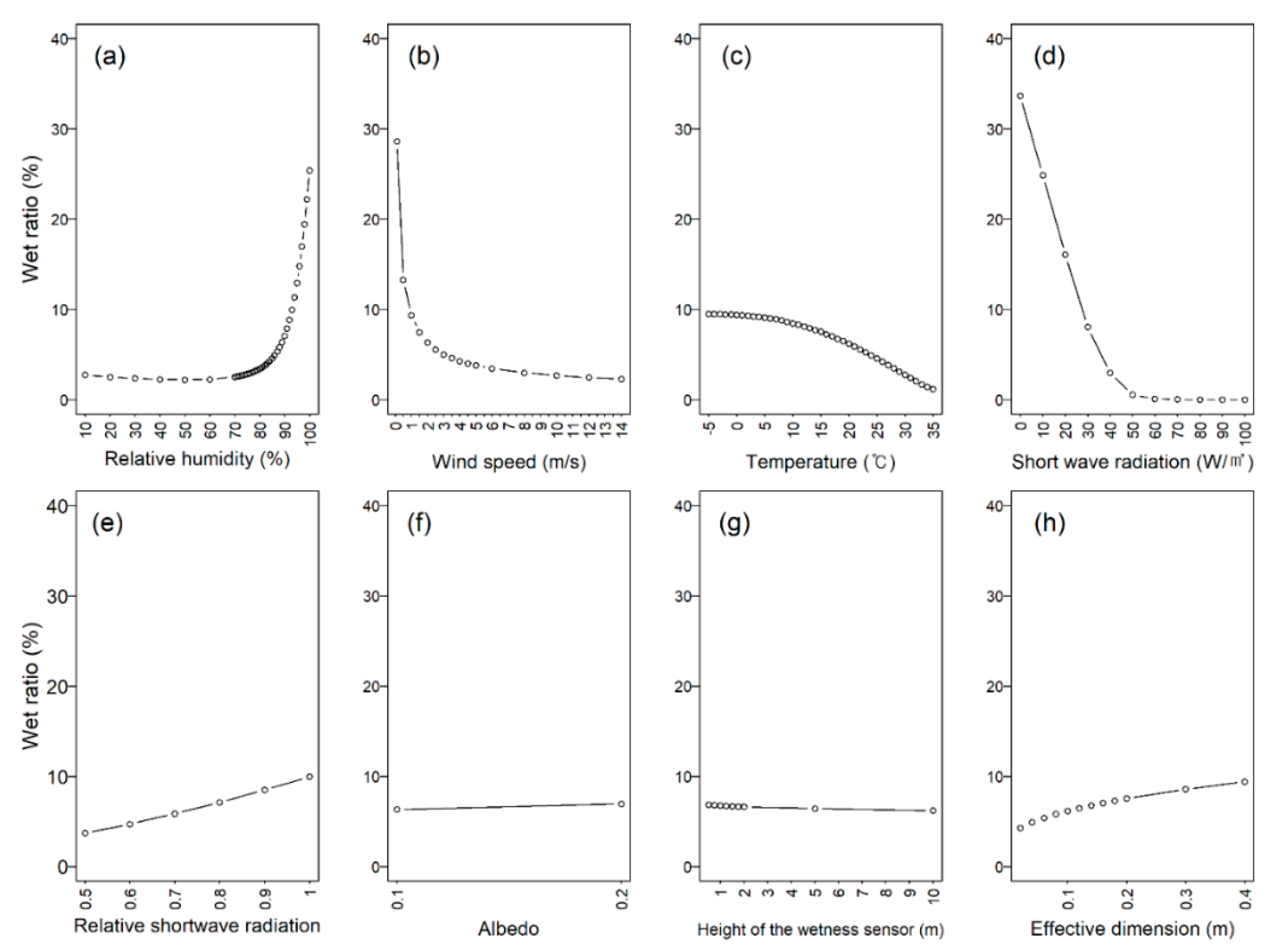
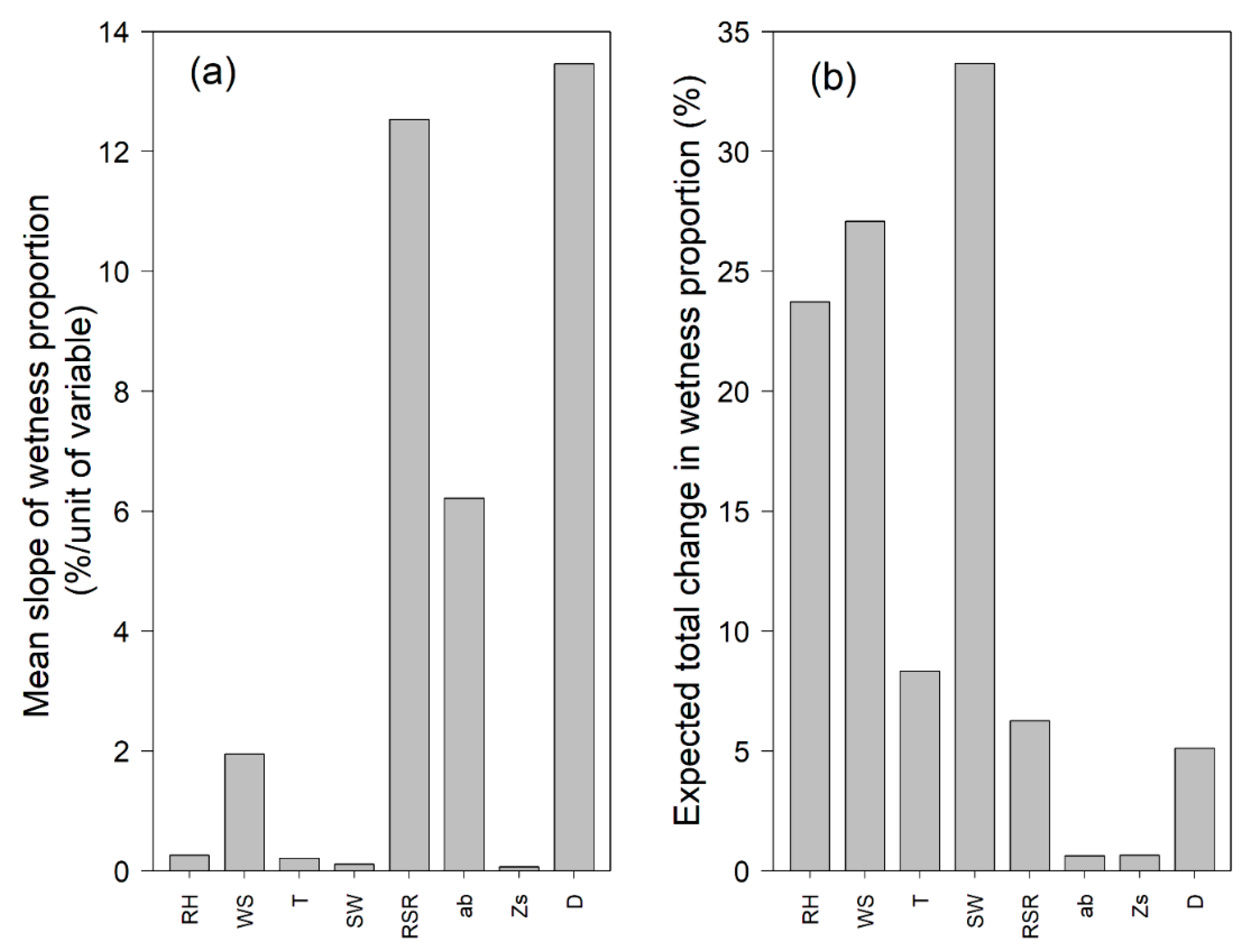
3.2. Sensitivity Analysis of PM Model and Performance Evaluation Results

The input data used in this study showed the LW behavior in accordance with the PM model input variable. This is because the input data represented various environmental conditions. To improve our understanding of LW estimation in the PM model, the sensitivity of input variables to LW estimation was roughly analyzed. As the systematical approach for investigating the sensitivity of the model was not employed, the results of sensitivity analysis in this study cannot fully present the sensitivity of the input variables for the PM model. The wetness proportions corresponding to specific input variable values were calculated and are presented in Figure 2. Based on the sensitivity analysis results, the wetness occurrence in the PM model was dominated by the meteorological variables. The largest change in the wetness proportion was demonstrated in SW (See Figure 2d). The three largest wetness proportion changes are observed in RH, WS, and SW. T may have produced the smallest impact on the wetness occurrence among the meteorological variables based on the PM model. Of the environmental and instrumental variables, RSR and D led to large changes in the wetness proportion within the tested variable ranges. Moreover, ab and $Z_s$ may have slightly influenced the wetness occurrence.

For a more detailed comparison, the impacts of the input variable on wetness were investigated. The mean slope of the wetness proportion in the PM model was considered to be the indicator representing the magnitude of the impact on the wetness. All input variables were calculated from the generated dataset. The mean slope estimates are presented in Figure 3a. It is shown that, based on the mean slope estimates, D, RSR, and ab have large values owing to the scales of these variables. To attenuate the scale effects on the input variable in the impact assessment, the expected total wetness proportion changes were calculated by multiplying the mean slope of the wetness proportion to the variable range.

For example, the mean slope value for RH and its range were approximately 0.264 and 90, respectively. The expected total change in the wetness proportion for RH was 23.7%. This means that the RH within the range could change by 23.7% in terms of the wetness proportion. Since this index represents the available change in the wetness proportion within a given range, the value of this index may account for the magnitude of impact on the wetness proportion within the given range. The expected total changes in the wetness proportion are presented in Figure 3b. The largest value of the expected total change is shown by SW, while WS and RH lead the second and third largest values for this index. The values of the expected total change for T, RSR, and D range from 5% to 10%, whereas ab and $Z_s$ lead to small changes in the wetness proportion within the range. Based on the sensitivity analysis results, SW, WS, and RH are the three most important input variables for determining the wetness occurrence in the PM model. T is also an important variable, although it has a smaller influence than the other meteorological variables.

Despite the influence of the environmental and instrumental variables on determining wetness, the meteorological variables were more important for this purpose in the PM model. To evaluate the LW estimation performance for the built emulators, the ACCs of the emulators built by the ML algorithm with different input variable sets were identified and are listed in

Table 3. Accuracies of emulators built by machine learning (ML) algorithm with different input variable sets. Note that the bold number indicates the largest accuracy among different models with the same input variable set.

Algorithms	M1	M2	M3	M4	M5	M6	M7	M8
ELM (E)	0.9537	0.8332	0.8178	0.7112	0.6978	0.6898	0.6701	0.6078
RF (R)	0.9357	0.8167	0.7974	0.7100	0.6919	0.6854	0.6637	0.6001
SVM (S)	0.9937	0.8415	0.8163	0.7181	0.6938	0.6911	0.6715	0.6012
DNN (D)	0.9927	0.8393	0.8168	0.7145	0.6985	0.6922	0.6731	0.6020

. Overall, SVM and DNN outperform the other ML algorithms, such as ELM and RF, in emulating the PM model. The differences between the ACCs of the employed ML algorithm become smaller when the number of input variables decreases. When the input variable that is the same as that of the PM model is used for the SVM and DNN, their ACCs are higher than 99%. For the M2 for which the input variable is set without SW, ab, and RSR, the SVM and RF provide higher ACC than the ELM and RF. The algorithm leading the highest ACC is SVM. For the M3, the ELM accuracy is the highest. As the number of input variables decreases, the emulator ACCs decrease. Unlike the sensitivity analysis results, the RH is apparently the most critical variable for determining the leaf wetness based on the ACC results for the emulators. When the RH is removed from the input variable set, the ACCs of the emulators largely decrease compared to the M2.

As shown in the results of the sensitivity analysis, T is the least important among T, WS, and RH. The smallest ACC decrease is shown when T is not used for the emulator input variable set compared to the other variables (see M2 and M3).

4. Case Study for Evaluation Based on Real-World Data

Although the PM model shows good performance and generality for LWD estimation, it has a limited ability to estimate LW and LWD because it mimics the real world. Thus, the results of a simulation study cannot represent the LW and LWD characteristics in the real world because they are based on the datasets generated by the PM model. Hence, to investigate the performances of the emulators in LWD estimation, they should be evaluated based on the observed LWD and meteorological variable data. In addition, the simulation results can demonstrate the performances of the emulators for LW estimation. Both accurate LW estimation and LWD estimation performance are important.

Hence, the performance of LWD estimation for the tested emulators should be investigated. As LWD is a continuous event, it needs to generate continuous meteorological variables for LWD generation based on the PM model. Simulating LWD by the PM model is difficult owing to the difficulties in generating realistic weather. A case study with real world data is mandatory to assess the performance of LWD estimation for emulators. Therefore, in this study, a case study was conducted to evaluate the performances of the tested emulators. Brief descriptions of the case study data and results are presented in the following subsections.

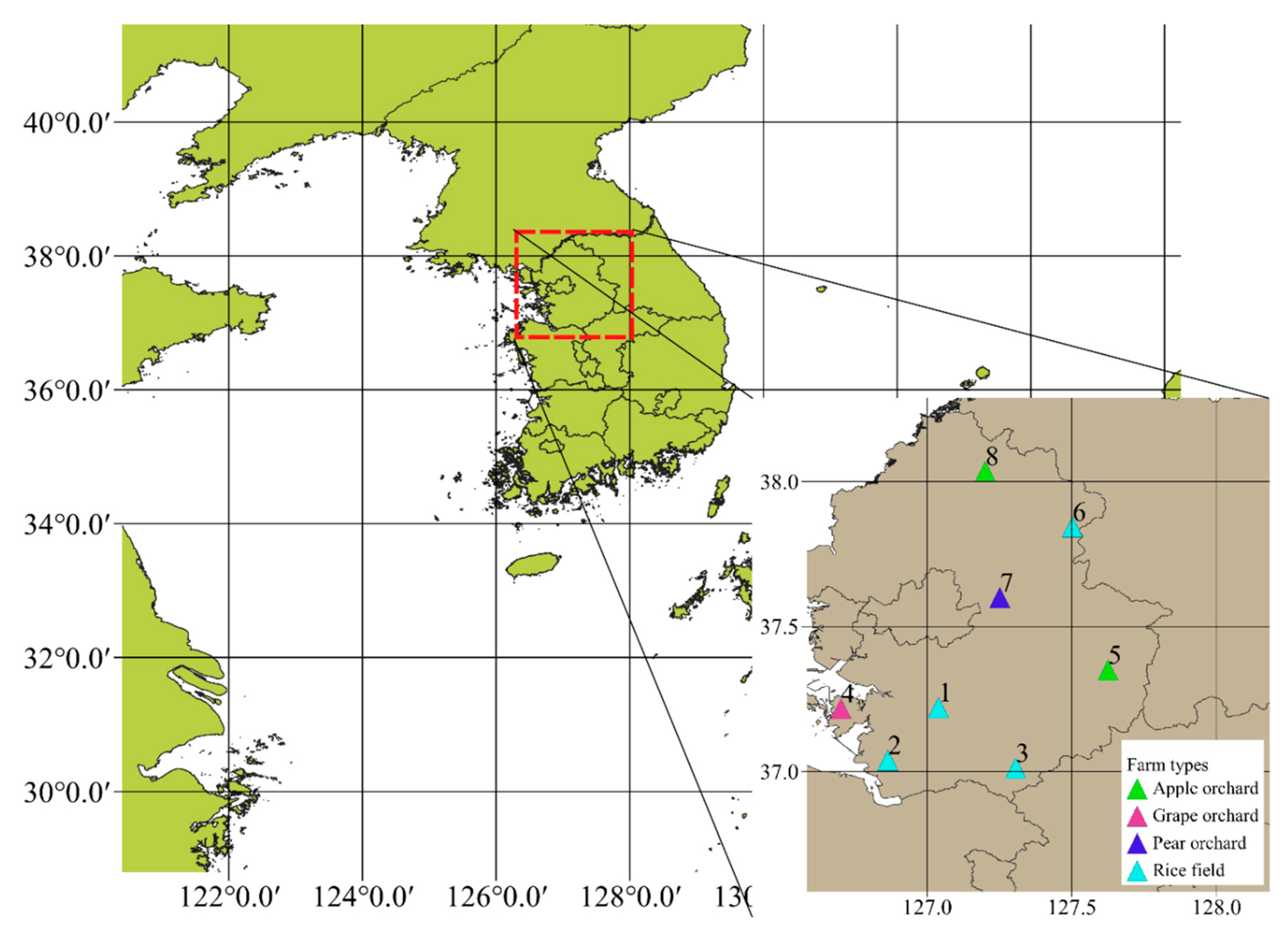
4.1. Data Description

The observed data, including LWD, T, RH, SW, and WS, were obtained from the Gyeonggi-do Agricultural Research & Extension Services of the Rural Development Administration. T and RH were measured at a 1.5 m height above the ground. Instruments for measuring short-wave radiation, WS, and LW were installed at a 2 m height above the ground. LW data were measured using two adjacent flat plate sensors (Model 237, Campbell Scientific) that were faced north at a 45° angle to the horizontal plane. Two LW sensors were used to detect the wetness and dryness conditions on a mock leaf. When any LW sensor detected wetness, the wetness was used for the LW data at the given moment. Weather data measured at eight farms, including those of apple, grape, and pear, as well as rice paddies, were employed. The data and location information are presented in

Table 4. Meteorological site data.

Site	Latitude (Degree)	Longitude (Degree)	Elevation (m)	Farm Type
1	37.221	127.039	45	Rice field
2	37.039	126.864	24	Rice field
3	37.012	127.306	34	Rice field
4	37.217	126.702	6	Grape orchard
5	37.350	127.625	57	Apple orchard
6	37.844	127.502	68	Rice field
7	37.600	127.251	65	Pear orchard
8	38.036	127.201	101	Apple orchard

and Figure 4, respectively. The temporal resolution of all data was hourly. The observed meteorological and LW data can be downloaded from the Gyeonggi-do Agricultural Research & Extension Services (https://nongupepi.gg.go.kr/). In this study, LWD is defined as the sum of LW from 0 to 23 h. The observed data from 2009 to 2017 were used, except for 2013 owing to a large amount of missing data from that year. Proportions of dryness and wetness for observed LW data are approximately 75% and 25%, respectively. The statistics of the observed meteorological variables are presented in

Table 5. Statistics of observed meteorological variables.

Statistics	T	RH	SW	WS
Mean	10.0	67.6	160.4	1.1
Standard deviation	11.8	22.3	239.6	1.3
Minimum	−26.2	10.0	0.0	0.0
Median	10.5	70.3	2.8	0.5
Maximum	36.9	100.0	1027.9	10.0

. The ranges of RH, T, SW, and WS are 10–100%, −26–37 °C, 0–1028 W/m², and 0–10 m/s, respectively. These ranges were apparently and adequately broad to cover various conditions of LW generations. Thus, these observed data were appropriate for identifying the characteristics of the emulators for LW and LWD estimation.

4.2. Results

DNN and SVM were selected because they showed good accuracy based on the simulation results. Models #2–#8 for DNN and SVM were employed for the PM model emulators. For a comparison, LW and LWD were estimated by using the PM model. In that estimation, ab and RSR were 0.2 and 1, respectively. The performances of LW estimation for the emulators using the DNN and SVM algorithms were assessed in terms of the accuracy, precision, recall, and F1 score. The boxplots of these evaluation measures for the given sites are presented in Figure 5.

Unlike the simulation results, the results of some of the emulators, e.g., M4 and M6, including RH and excluding WS, are better than that of the PM model. These emulators outperform the other emulators and the PM model. The other emulators show similar performances, as demonstrated by the simulation results. The highest mean accuracy value for LW estimation is observed in D4, that is, DNN with M4 (0.847). S6 and D6 provide the second and third highest accuracies (0.842 and 0.840) among the employed models. The mean accuracy for the PM model is the fifth highest; its value is approximately 0.752. The D4, D6, S4, and S6 models provide higher precision than the other models, while PM and the other models show higher recall values than the D4, D6, S4, and S6 models. With respect to the F1 score, D4 model has the largest F score. Those of the other emulators are lower than that of the PM model.

Although the emulator performance for LW estimation can indicate the LWD estimation performance, their performances differ. Thus, the performances of the employed emulators for estimating LWD were evaluated based on the Pearson correlation, RMSE, MAE, and MBE. The boxplots of these evaluation measures for all employed sites, emulators, and the PM model are presented in Figure 6. Overall, D4, D6, S4, and S6 show good performances. Additionally, they provide better LWD estimation performance than the PM model. Based on the Pearson correlation of the LWD estimation, D3, D4, D6, S2, S3, S4, and S6 lead to higher values than the PM model. D4, D6, S4, and S6 have smaller values of RMSE and MAE than the PM model, whereas the other emulators do not. D4, D6, S4, and S6 underestimate LWD, whereas the others overestimate LWD.

5. Discussion

Based on the results of the simulation and case studies, it can be concluded that the ML algorithm can properly emulate the PM model in LW and LWD estimations. The emulators that use the M2 input variable set realize ~84% ACC of the PM model for LW estimation. In the case of the M3 input variable, the emulators can realize ~81% ACC of the PM model. Although the emulators cannot copy the PM model perfectly, the performance of the emulators may be good. Thus, these emulators may be good alternatives to estimate LW in which limited meteorological variables are available. In the case study for the LWD data in South Korea, the emulators provide comparable performances to the PM model for estimating LW and LWD. For LW estimation, the emulators using M2 and M3 show similar performances to the PM model. Additionally, some emulators that use RH for input variable realize better performances than the PM model in the case study for LW and LWD estimations.

In the current study, 32 combinations using four ML algorithms and eight input variable sets are tested for the emulator of the PM model. Of the 32 combinations, the DNN using M4 (D4) is considered to be the most appropriate combination of the ML algorithm and input variable set. This DNN is the best emulator based on the results of the case study; it uses RH and T for input variables. D4 realizes better LW and LWD estimations for the employed LWD observations. However, the results of the case study are only valid for the LWD observations used in this study. Environmental conditions and the main generating mechanisms for LW differ depending on locations. Hence, the results of the case study would be different in other locations. Wilks and Shen [13] suggested an RH-threshold-based model for LWD estimation. Some studies reported that the RH-threshold model realizes a good performance in various regions; however, the model needs to be calibrated [12,41,42]. Park et al. [25] reported that the RH-threshold-based LWD estimation model led to the best performance except for the ones based on ML. In addition, Gao et al. [43] showed that an RH-threshold-based LWD estimation model would be the best model among the LWD estimation models tested in their study because it uses only one variable to estimate LWD. As the RH-threshold-based LWD estimation model performs well for many regions, there is a high possibility that D4 may provide a good performance in other regions.

Sensitivity analysis of the PM model for input variables may represent the magnitude of importance given for an input variable in the LW estimation of the PM model. The results of the sensitivity analysis are consistent with another study [43]. According to the results of the sensitivity analysis, SW and WS may be critical variables for determining the occurrence of wetness. This result indicates that D2, D3, S2, or S3 may be the best emulator among the tested emulators in the case study if the results of the sensitivity analysis are correct. However, D4, which does not use SW and WS, is the best emulator in the case study. This leads to the inference that there is a discrepancy between the results of the simulation and case studies.

Increments of magnitude for SW and WS lead to a decrease in the LW frequency, while increasing RH leads to an increment of the LW frequency. The RH value governs the occurrence of wetness, and WS suppresses the existence of wetness on the surface. As shown in Figure 5, D4 and D6 have high precisions, while their recalls are low, and they have negative bias (see Figure 6). These results imply that D4 and D6 using RH determine wetness when the probability of wetness occurrence is significantly high. By contrast, wetness is estimated in D2 and D3 using WS when the probability of wetness occurrence is low. Hence, the recalls of D2 and D3 are higher than D4 and D6. As high WS suppresses the occurrence of wetness, overestimating the wetness of D2 and D3 may indicate that the value of the WS data is considered smaller than the actual value in the PM model. This can be caused by two reasons: (1) the WS interpolation scheme in the PM model is inappropriate for the data used in the case study and (2) measuring accuracy of the used WS data is poor. As LW was consistently overestimated for all sites, the interpolation scheme does not work properly. The WMO recommended that the measuring accuracy of the WS data is less than $\pm$0.5m/s [44,45]. As shown in Figure 3, wetness proportion is drastically changed from 0 to 1 m/s. As the WS in this range plays a critical role in estimating LW, the limited measurement accuracy of WS also limits the accuracy of LW estimation. Hence, the poor performances of D2 and D3 for LW and LWD estimation may be as a result of the limitations of WS measurement. To improve LWD estimation using meteorological variables, WS data with high accuracy should be employed. This discussion highlights that the use of many meteorological variables elevates the uncertainty in LW and LWD estimation. For example, Gao et al. [43] reported that an RH-threshold-based LWD estimation model provided a comparable performance to an ML-based LWD estimation model using a large number of input variables. Hence, parsimony is strongly recommended in developing LWD estimation models using meteorological variables.

Some emulators of the PM model provided better performance in LW and LWD estimation than the PM model based on the results of the case study. Based on the results of the simulation study, the PM model would be better than the emulators. As mentioned in the previous paragraph, the wind speed data have large uncertainty in LW estimation. Other meteorological observations also have uncertainty. The ab and RSR in the PM model were indirectly obtained. In this study, the value of ab was obtained based on the type of vegetation. However, ab is changed depending on the season. Even this value can be changed based on the condition of the leaf surface. Therefore, this uncertainty of parameters in the PM model can propagate errors in the LW estimation of the physical model. Thus, the results of the case study can be changed by the quality of the observed data.

Using the same hyperparameters for input variable sets can lead to a decrease in performance of the ML algorithm. In this study, when a regularization such as the layer normalization and mini-batch was not adopted, the performances of the emulators by DNN showed large differences depending on the input variable set. However, when the regularization method was applied and the number of layers and nodes was large enough, the performances of emulators with different hyperparameters were very similar. Their performances were not the same, but the difference between them would be so small as to be neglectable. Regularization tunes the strengths of the node and this provides good performance with a structure with a large complexity. So, even if different input variable sets are employed in the DNN, the emulators can provide good performances because the structure of the DNN is complex enough. Since the regularization was employed in the current study, we employed the same hyperparameters, which can lead to good performance for different input variable sets, to emulators with different input variable sets. Therefore, the performance of the emulators in the DNN is not the best and these can become better by tuning hyperparameters.

6. Conclusions

This study developed emulators of the PM model using ML techniques and investigated the performance of emulators based on simulation and case studies. The following conclusions can be made from the current study:

(1)

The emulators for the physical model can be applicable for LW and LWD estimation. The emulators using RH, WS, T, Z_s, and D provide approximately 84% ACC of the PM model for LW estimation. In addition, the emulators using RH, WS, Z_s, and D provide approximately 81% ACC of the PM model.

(2)

Some emulators that use RH for input variable realize better performances than the PM model in the case study for LW and LWD estimations. The emulator using RH, T, Z_s, and D leads to the best performance based on the case study. The discrepancy between the simulation and case studies may be induced by the uncertainty in the observed data.

(3)

DNN and SVM algorithms can be good techniques for emulating the PM model in LW and LWD estimation. The two techniques provide slightly better performances than other used ML algorithms, particularly in applications with a larger number of input variables.

References

1. Sentelhas, P.C.; Gillespie, T.J.; Gleason, M.L.; Monteiro, J.E.B.A.; Helland, S.T. Operational exposure of leaf wetness sensors. Agric. For. Meteorol. 2004, 126, 59–72. [Google Scholar] [CrossRef]
2. Huber, L.; Gillespie, T.J. Modeling Leaf Wetness in Relation to Plant Disease Epidemiology. Annu. Rev. Phytopathol. 1992, 30, 553–577. [Google Scholar] [CrossRef]
3. Schmitz, H.F.; Grant, R.H. Precipitation and dew in a soybean canopy: Spatial variations in leaf wetness and implications for Phakopsora pachyrhizi infection. Agric. For. Meteorol. 2009, 149, 1621–1627. [Google Scholar] [CrossRef]
4. Jesperson, G.D.; Sutton, J.C. Evaluation of a forecaster for downy mildew of onion (Allium cepa L.). Crop Prot. 1987, 6, 95–103. [Google Scholar] [CrossRef]
5. de Visser, C.L.M. Development of a Downy Mildew Advisory Model Based on Downcast. Eur. J. Plant Pathol. 1998, 104, 933–943. [Google Scholar] [CrossRef]
6. Wang, H.; Sanchez-Molina, J.A.; Li, M.; Berenguel, M. Development of an empirical tomato crop disease model: A case study on gray leaf spot. Eur. J. Plant Pathol. 2020, 156, 477–490. [Google Scholar] [CrossRef]
7. Magarey, R.D.; Russo, J.M.; Seem, R.C. Simulation of surface wetness with a water budget and energy balance approach. Agric. For. Meteorol. 2006, 139, 373–381. [Google Scholar] [CrossRef]
8. Pedro, M.J.; Gillespie, T.J. Estimating dew duration. II. Utilizing standard weather station data. Agric. Meteorol. 1981, 25, 297–310. [Google Scholar] [CrossRef]
9. Pedro, M.J.; Gillespie, T.J. Estimating dew duration. I. Utilizing micrometeorological data. Agric. Meteorol. 1981, 25, 283–296. [Google Scholar] [CrossRef]
10. Kim, K.S.; Taylor, S.E.; Gleason, M.L. Development and validation of a leaf wetness duration model using a fuzzy logic system. Agric. For. Meteorol. 2004, 127, 53–64. [Google Scholar] [CrossRef]
11. Marta, A.D.; De Vincenzi, M.; Dietrich, S.; Orlandini, S. Neural network for the estimation of leaf wetness duration: Application to a Plasmopara viticola infection forecasting. Phys. Chem. Earth 2005, 30, 91–96. [Google Scholar] [CrossRef]
12. Sentelhas, P.C.; Dalla Marta, A.; Orlandini, S.; Santos, E.A.; Gillespie, T.J.; Gleason, M.L. Suitability of relative humidity as an estimator of leaf wetness duration. Agric. For. Meteorol. 2008, 148, 392–400. [Google Scholar] [CrossRef]
13. Wilks, D.S.; Shen, K.W. Threshold Relative Humidity Duration Forecasts for Plant Disease Prediction. J. Appl. Meteorol. 1991, 30, 463–477. [Google Scholar] [CrossRef] [Green Version]
14. Francl, L.J.; Panigrahi, S. Artificial neural network models of wheat leaf wetness. Agric. For. Meteorol. 1997, 88, 57–65. [Google Scholar] [CrossRef]
15. Gillespie, T.J.; Srivastava, B.; Pitblado, R.E. Using Operational Weather Data to Schedule Fungicide Sprays on Tomatoes in Southern Ontario, Canada. J. Appl. Meteorol. 1993, 32, 567–573. [Google Scholar] [CrossRef] [Green Version]
16. Gleason, M.; Taylor, S.; Loughin, T.; Koehler, K. Development and validation of an empirical model to estimate the duration of dew periods. Plant Dis. 1994. [Google Scholar] [CrossRef]
17. Rao, P.S.; Gillespie, T.J.; Schaafsma, A.W. Estimating wetness duration on maize ears from meteorological observations. Can. J. Soil Sci. 1998, 78, 149–154. [Google Scholar] [CrossRef]
18. Sentelhas, P.C.; Gillespie, T.J.; Gleason, M.L.; Monteiro, J.E.B.M.; Pezzopane, J.R.M.; Pedro, M.J. Evaluation of a Penman–Monteith approach to provide “reference” and crop canopy leaf wetness duration estimates. Agric. For. Meteorol. 2006, 141, 105–117. [Google Scholar] [CrossRef]
19. Monteith, J.L.; Unsworth, M.H. (Eds.) Principles of Environmental Physics. In Principles of Environmental Physics, 4th ed.; Academic Press: Boston, MA, USA, 2013; p. iii. [Google Scholar] [CrossRef]
20. Allen, R.G.; Pereira, L.S.; Raes, D.; Smith, M. Crop Evapotranspiration-Guidelines for Computing Crop Water Requirements-FAO Irrigation and Drainage Paper 56; FAO: Rome, Italy, 1998; Volume 300, p. D05109. [Google Scholar]
21. Walter, I.A.; Allen, R.G.; Elliott, R.; Jensen, M.E.; Itenfisu, D.; Mecham, B.; Howell, T.A.; Snyder, R.; Brown, P.; Echings, S.; et al. ASCE’s Standardized Reference Evapotranspiration Equation. In Watershed Management and Operations Management 2000; American Society of Civil Engineers: Reston, VA, USA, 2001. [Google Scholar] [CrossRef]
22. Niazian, M.; Niedbała, G. Machine Learning for Plant Breeding and Biotechnology. Agriculture 2020, 10, 436. [Google Scholar] [CrossRef]
23. Niedbała, G.; Kurasiak-Popowska, D.; Stuper-Szablewska, K.; Nawracała, J. Application of Artificial Neural Networks to Analyze the Concentration of Ferulic Acid, Deoxynivalenol, and Nivalenol in Winter Wheat Grain. Agriculture 2020, 10, 127. [Google Scholar] [CrossRef] [Green Version]
24. Yin, H.; Gu, Y.H.; Park, C.-J.; Park, J.-H.; Yoo, S.J. Transfer Learning-Based Search Model for Hot Pepper Diseases and Pests. Agriculture 2020, 10, 439. [Google Scholar] [CrossRef]
25. Park, J.; Shin, J.-Y.; Kim, K.R.; Ha, J.-C. Leaf Wetness Duration Models Using Advanced Machine Learning Algorithms: Application to Farms in Gyeonggi Province, South Korea. Water 2019, 11, 1878. [Google Scholar] [CrossRef] [Green Version]
26. Shin, J.-Y.; Kim, B.-Y.; Park, J.; Kim, K.R.; Cha, J.W. Prediction of Leaf Wetness Duration Using Geostationary Satellite Observations and Machine Learning Algorithms. Remote Sens. 2020, 12, 3076. [Google Scholar] [CrossRef]
27. Huang, G.-B.; Zhu, Q.-Y.; Siew, C.-K. Extreme learning machine: Theory and applications. Neurocomputing 2006, 70, 489–501. [Google Scholar] [CrossRef]
28. Peña, M.; van den Dool, H. Consolidation of Multimodel Forecasts by Ridge Regression: Application to Pacific Sea Surface Temperature. J. Clim. 2008, 21, 6521–6538. [Google Scholar] [CrossRef] [Green Version]
29. Huang, G.; Zhou, H.; Ding, X.; Zhang, R. Extreme Learning Machine for Regression and Multiclass Classification. IEEE Trans. Syst. Man Cybern. Part B 2012, 42, 513–529. [Google Scholar] [CrossRef] [Green Version]
30. Pal, M. Random forest classifier for remote sensing classification. Int. J. Remote Sens. 2005, 26, 217–222. [Google Scholar] [CrossRef]
31. Smith, A. Image segmentation scale parameter optimization and land cover classification using the Random Forest algorithm. J. Spat. Sci. 2010, 55, 69–79. [Google Scholar] [CrossRef]
32. Breiman, L. Random Forests. Mach. Learn. 2001, 45, 5–32. [Google Scholar] [CrossRef] [Green Version]
33. Wright, M.N.; Ziegler, A. ranger: A Fast Implementation of Random Forests for High Dimensional Data in C++ and R. arXiv 2017, 77, 17. [Google Scholar] [CrossRef] [Green Version]
34. Jung, K.; Shin, J.-Y.; Park, D. A new approach for river network classification based on the beta distribution of tributary junction angles. J. Hydrol. 2019, 572, 66–74. [Google Scholar] [CrossRef]
35. Chen, P.-H.; Lin, C.-J.; Schölkopf, B. A tutorial on ν-support vector machines. Appl. Stoch. Model. Bus. 2005, 21, 111–136. [Google Scholar] [CrossRef]
36. Bergstra, J.; Bardenet, R.; Bengio, Y.; Kégl, B. Algorithms for hyper-parameter optimization. In Proceedings of the 24th International Conference on Neural Information Processing Systems, Granada, Spain, 12–14 December 2011; pp. 2546–2554. [Google Scholar]
37. Tran, T.T.K.; Lee, T.; Shin, J.-Y.; Kim, J.-S.; Kamruzzaman, M. Deep Learning-Based Maximum Temperature Forecasting Assisted with Meta-Learning for Hyperparameter Optimization. Atmosphere 2020, 11, 487. [Google Scholar] [CrossRef]
38. Xu, J.; Sun, X.; Zhang, Z.; Zhao, G.; Lin, J. Understanding and Improving Layer Normalization. In Proceedings of the Advances in Neural Information Processing Systems, Vancouver, BC, Canada, 27–30 November 2019; pp. 4381–4391. [Google Scholar]
39. Kingma, D.P.; Ba, J. Adam: A method for stochastic optimization. arXiv 2014, arXiv:1412.6980. [Google Scholar]
40. Paszke, A.; Gross, S.; Massa, F.; Lerer, A.; Bradbury, J.; Chanan, G.; Killeen, T.; Lin, Z.; Gimelshein, N.; Antiga, L. Pytorch: An imperative style, high-performance deep learning library. In Proceedings of the Advances in Neural Information Processing Systems, Vancouver, BC, Canada, 8–14 December 2019; pp. 8026–8037. [Google Scholar]
41. Magarey, R.D.; Isard, S.A. A Troubleshooting Guide for Mechanistic Plant Pest Forecast Models. J. Integr. Pest Manag. 2017, 8. [Google Scholar] [CrossRef]
42. Bassimba, D.D.M.; Intrigliolo, D.S.; Dalla Marta, A.; Orlandini, S.; Vicent, A. Leaf wetness duration in irrigated citrus orchards in the Mediterranean climate conditions. Agric. For. Meteorol. 2017, 234–235, 182–195. [Google Scholar] [CrossRef]
43. Gao, Z.; Shi, W.; Wang, X.; Cao, B.; Wang, Y. Comparison of the performance of leaf wetness duration models for rainfed jujube (Ziziphus jujuba Mill.) plantations in the loess hilly region of China using machine learning. Ecohydrology 2020, 13, e2237. [Google Scholar] [CrossRef]
44. Gommes, R.; Challinor, A.; Das, H.; Dawod, M.; Mariani, L.; Tychon, B.; Krüger, R.; Otte, U.; Vega, R.; Trampf, W. Guide to Agricultural Meteorological Practices; World Meteorological Organization: Geneva, Switzerland, 2010; Volume 134. [Google Scholar]
45. WMO. Guide to Instruments and Methods of Observation; World Meteorological Organisation: Geneva, Switzerland, 2018. [Google Scholar]
Figure 1. Structure of deep neural network (DNN) model for the leaf wetness (LW) estimation emulator based on the PM model.
Agronomy 11 00216 g001
Figure 2. Wetness proportions in accordance with the input variable values; (a) RH, (b) WS, (c) T, (d) SW, (e) RSR, (f) ab, (g) Z s , and (h) D.
Agronomy 11 00216 g002
Figure 3. Mean slope of wetness proportion (a) and expected total change (b) in wetness proportion for the input variables in the PM model.
Agronomy 11 00216 g003
Figure 4. Locations of weather measuring sites.
Agronomy 11 00216 g004
Figure 5. Accuracy, precision, recall, and F1 score of leaf wetness duration (LWD) estimates by employed models. Note Table 2. D8 and S2–S8 indicate DNN-based models #2–#8 and SVM-based models #2–#8, respectively.
Agronomy 11 00216 g005
Figure 6. Correlation, RMSE, MAE, and MBE of LWD estimates by employed models. Note that D2–D8 and S2–S8 indicate DNN-based models #2 to #8 and SVM-based models #2–#8, respectively.
Agronomy 11 00216 g006