Mapping Spatial Management Zones of Salt-Affected Soils in Arid Region: A Case Study in the East of the Nile Delta, Egypt

Abstract

Soil salinization is a global problem that affects a large part of the world, especially arid and semi-arid regions. Hence, diagnosing soil salinity is the first step towards appropriate management. The current work aims to assess and map soil salinity in the eastern Nile Delta using principal component analysis (PCA). In order to develop appropriate solutions for rational management to mitigate the impacts of soil salinization and increase yield production 34 soil profiles were dug that covered the variation in the soils located at the northeast of the Nile delta. The spatial variation of soil parameters was mapped using ordinary kriging interpolation. The results of PCA illustrated that, among the studied soil properties, soil electrical conductivity (ECe), sodium adsorption ratio (SAR), exchangeable sodium percent (ESP), and bulk density (BD), are the critical factors affecting management practices in the Nile Delta. Two spatial management zones (SMZ) were identified; SMZ 1 occupied 45.04% of the study area and SMZ2 occupied 54.96% of the study area. The average of soil pH, ECe, SAR, CEC, ESP and BD were 8.31, 20.32 dSm⁻¹, 47.19, 32.9 cmolckg⁻¹, 32.85% and 1.47 Mgm⁻³ for the first cluster (SMZ1), respectively. In addition, the second cluster (SMZ2) had average soil pH, ECe, SAR, CEC, ESP and BD of 7.75, 12.30 dSm⁻¹, 26.6, 25.23 cmolckg⁻¹, 26.6% and 1.27 Mgm⁻³. The results showed p-value < 0.05 which confirms that there is a significant statistical difference between the two zones. Finally, the results obtained could be used as a fundamental basis for improving agricultural management practices in such salt-affected soils.

1. Introduction

Increasing of food demand represents a great pressure on governments, especially in third world countries, as a result of the high population increase, which has led to increased competition over natural resources use [1,2,3,4]. There are many factors that cause land degradation, such as urban sprawl, soil salinization, soil waterlogging and soil compaction, as well as mismanagement of land use [5,6,7,8]. Salt-affected soils are spread in various areas of the world, as approximately 6% of the total world’s soils are affected by salinity, and they are associated to many factors regarding the region’s climate, such as temperature, amount of rain in addition other factors such soil characteristics, saline groundwater and etc. [9,10]. In addition, some studies indicate that about 20% of irrigated soils around the world suffer from ongoing salinization processes [11]. Soil salinization is considered one of the main challenges that hinder agricultural production in arid and semi-arid areas [12]. Increasing the concentration of soluble salts in the soil by more than 4 dSm⁻¹ influences plant growth and is certainly reflected in the quantity and quality of the crop in many areas around the world [13,14,15]. The increase of salts concentration in the root zoon especially the ions of Na⁺, Cl⁻, Mg²⁺, SO4₂⁻ or HCO₃⁻ causes toxicity to cross, moreover it affects the inhibition of biochemical and physiological processes as well as disrupting the metabolism and oxidation and reduction reactions inside the plant cell, thus disrupting water and nutrients uptake, the development of crop growth and the spread of the roots inside the soil [16]. Soil salinization is affected by many natural processes such as geological sedimentation or physicochemical factors such as erosion, as well as human practices which determine the direction soil salinization [17]. In order to improve the management of salt-affected lands, we must understand the type of salts that are prevalent as well as their spatial distribution to make appropriate plans for soil salinization management and mitigate their impacts [18,19]. Soils of lakes in arid and semi-arid areas worldwide suffer from ongoing salinization processes, the soil of Idku and Manzala lakes in the Nile delta effected by rising groundwater level that characterized by high brackish ranging between 1–69 dSm⁻¹ in south Idku [20] in may reach more than 100 dSm⁻¹ south Manzala lake [21]. The soils of Urmia hypersaline Lake are characterized by wide range of soil salinity from 0.67 to 155 dSm⁻¹ [22]. Remote-sensing data have been used during past decades to monitor the change of soil and crop conditions. The normalized difference vegetation index (NDVI) was most often used to describe vegetation status. This index depends on healthy plant absorbs most of the red light, while reflecting most of the near-infrared light, this index values ranging between −1 to 1 as the index values increase with increasing greenness and the health status of the plant [23]. This indicator has been widely used in many studies, as some authors have used NDVI for crop quantities [24], monitoring agricultural management and as an indicator of soil fertility status [25]. On the other hand, NDVI was used as an indicator of some degradation factors such as soil salinity [26].

One of the important research topics of precision agriculture is site-specific management zones [27] which can be defined as the division of heterogeneous lands into units homogeneous in their characteristics [28,29]. By identifying the management zones, it can control the rates of fertilizers as well as irrigation operations, and this is reflected in increased economic profit, reduced environmental risks, and achieving the purpose of “precise management” [30]. Identification of sub-field areas is difficult due to spatial variability and the dynamic interactions of the potential factors that may influence crop productivity [31,32]. There is an urgent need to understand the relationship between soil properties based on multivariate analysis and geostatistical analysis [19,33].

Most importantly, the PCA can be used for soil evaluation in a fast and cost-effective methodology and is also suitable for any stages of the land management program [34]. The PCA has many advantages as follows: (1) it removes correlated features: if an independent variable is correlated with one or more of the other independent variables in a multiple regression equation, causes multicollinearity that undermines the statistical significance of an independent variable [35], and after running the PCA on the dataset all the PCs are independent of one another, i.e., there is no correlation between them [35]; (2) it improves algorithm performance: having too many features in the models significantly degrades the algorithms. PCA is a very common method to reduce the number of features in the dataset through identifying the most important PCs that explain maximum information about the dataset. Therefore, using PCA to speed up the algorithm is a reasonable choice [36]; (3) it reduces overfitting: PCA helps in overcoming the overfitting issue through minimizing the number of variables in the dataset [37]; and (4) it improves visualization: it is very hard to visualize and understand the data in high dimensions. PCA transforms high-dimensional data into low-dimensional data (two dimensions) so that it can be visualized easily [38]. PCA is often used to make data easy to explore and visualize [39].

Li et al. [40] used the fuzzy clustering analysis to delineate the site-specific management zones in coastal saline soils. The authors found that the optimal number of management zones for their study area was three. In addition, there were significant statistical differences between the chemical soil properties and yield production in each management zone. Delineation of management zones of soil apparent electrical conductivity in the southeastern pampas was studied by Peralta et al. [41] who reported that EC values successfully delimited three homogeneous soil zones associated with spatial distribution of clay, soil moisture, CEC, SOM content and pH. These results suggested that field-scale EC maps have the potential to design sampling zones to implement site-specific management strategies. Molin and Castro [42] mentioned that the utility of electrical conductivity in the definition of management zones and the feasibility of the proposed method is affective. Metwally et al. [43] used PCA and clustering to delineate site-specific management zones based on soil fertility and they recommended using this methodology for management zones. Hence this method could be used effectively for soil site-specific nutrient management for avoiding soil degradation concurrently with maximizing crop production.

Soil salinization and land degradation in Egypt is considered a complex problem that is linked to many factors; heterogeneous soil properties, climate conditions, saline groundwater that rises to the soil surface, and human activities. Hence, the application of traditional methodologies may not give the desired results that can be applied at the field level. Therefore, multivariate analysis that has advantages over other methods as it is permissible to integrate many factors in the analysis [33]. The main objectives of this study were: (1) mapping the spatial variability of the soil properties east of Nile Delta, (2) delineating the spatial management zones of salt-affected soil in some arid regions, and (3) suggesting alternative solutions to mitigate the impacts of land salinization.

2. Materials and Methods

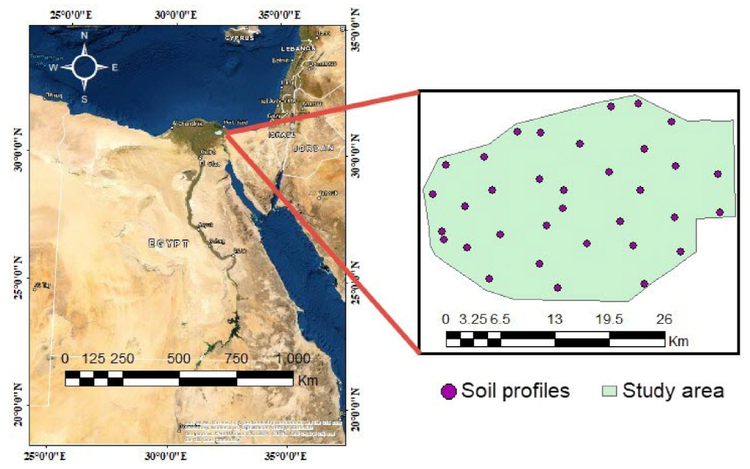
2.1. Description of the Study Area

The study area is located in east of Nile Delta between longitude 31°55′–32°12′ East longitude and 30°59′–31°5′ north latitude (Figure 1). The study area occupies about 75,980 hectares. The area is exposed to activation of salinization processes as a result of several factors such as high levels of the saline water table that seeps from El-Manzala Lake. In addition, the high temperature in the summer season, accelerate the formation of thin layers of salt on the surface soils [7]. In addition, the human factor is considered one of the most important factors in influencing the formation of the salt-affected soils in the Nile Delta. The study area is characterized by a hot arid to semi-arid climate, warm with winter rainfall. The average annual temperature is about 30° according to Port Said metrological station during 2000–2015, in addition the area receives a low amount of rain where the annual rainfall is 71 mm. Based on Taxonomy [44] the soil temperature regime of the studied area could be defined as thermic and soil moisture regime as torric, except for the soil which has a high water table, the soil moisture regime could be considered as aquic. The study area is a lacustrine plain, where it deposits were formed by siltation that occurred in El-Manzala Lake forming its salty bed [45].

2.2. Field Work and Laboratory Analyses

A reconnaissance soil survey was conducted throughout the investigated area in order to identify soil and crop patterns in addition, landscape characteristic. Based on the pre-field interpretation and the information gained during the reconnaissance survey a randomly 34 georeferenced soil profiles were created covering the study area (Figure 1). The depth of the soil profiles depended on the presence of hard rock, hardpan, permanent water. Eighty four soil samples were collected from surface and subsurface layers. The samples collected from each soil profile were mixed and transferred to a polythene bag and labeled. Each composite sample was prepared for laboratory analysis by being air-dried, crushed, grinded well and passed through a sieve with a hole diameter of 2 mm. All prepared composite samples were analyzed according to the methods described by Richards [46] and Van [47]. Soil electrical conductivity (EC_e) was measured in soil paste extract at 25 °C using an EC-meter after calibrating the device with standard KCl solution (0.01 m). Soil pH was measured in soil-water suspension (1:2.5) at 25 at 25 °C using a pH-meter with glass electrode after calibrating the device with standard pH buffer solutions (acid (pH = 4), neutral (pH = 7) and alkaline (pH = 9)). The soluble sodium and potassium ions were measured in a soil paste extract using a flame-photometer device and interpolation the galvanometer readings of device using a standard curve of sodium and potassium. The soluble calcium and magnesium ions were measured in soil paste extract using titration with a standard solution of EDTA (ethylenediaminetetraacetic acid) after pH was adjusted to 12 using sodium hydroxide solution in the case of calcium in the presence of ammonium purpurate (murexide) indicator until the end point (the color change from red to lavender or purple.) and to 10 using ammonia buffer solution in the case of calcium + magnesium in the presence of eriochrome black indicator until the end point (the color changes from red to blue); finally, the magnesium was computed by subtracting calcium from the calcium + magnesium. The sodium adsorption ratio (SAR) was computed using the following equation:

$$SAR=\frac{Na}{\sqrt{\frac{Ca+Mg}{2}}}$$

where Na⁺, Ca²⁺ and Mg²⁺ are soluble sodium, calcium and magnesium respectively and the concentration of them expressed as mmolcL⁻¹. The chloride ions were measured in soil paste extract using titration with standard silver nitrate (AgNO₃) solution in the presence of potassium chromate (K₂CrO₄) indicator until the end point that occurs when all the chloride ions are precipitated and then additional silver ions react with the chromate ions of the indicator, potassium chromate, to form a reddish-brown precipitate of silver chromate. The carbonate and bicarbonate ions were measured in soil paste extract using titration with standard sulphuric acid (H₂SO₄) solution in the presence of phenolphthalein indicator until the end point (colorless) in the case of carbonate ions and methyl orange indicator until the end point (orange color) in the case of bicarbonate. Soil organic carbon (OC) was determined using the Walkley–Black method which depends on the oxidation of organic carbon by concentrated sulfuric acid in the presence of an excess of potassium bichromate (K₂Cr₂O₇) solution and then titration of the excess of potassium bichromate with a standard solution of ferrous ammonium sulfate (Fe (NH₄)₂ (SO₄)₂.6H₂O) in the presence of diphenylamine indicator until reaching the end point (green color appears). The percent of soil organic matter was computed as OC% × 1.71. The soil calcium carbonate (CaCO₃) was determined using the volumetric calcimeter method where the carbonate is treated with an excess acid and the CO₂ is determined volumetrically. Exchangeable cations were extracted using 1 N ammonium acetate solution at pH 7 and then the flame-photometer device was used to determine exchangeable sodium and exchangeable potassium where exchangeable calcium and exchangeable magnesium were determined using titration with standard solution of EDTA. Cation exchange capacity (CEC) was determined using the centrifuge method which depends on saturating the sample with sodium by treating it with sodium acetate solution (1 N) and then replacing the adsorbed sodium from the sample by extraction with ammonium acetate solution (1 N) and determining it using a flame-photometer. Soil bulk density was determined using the paraffin wax-coated clod method.

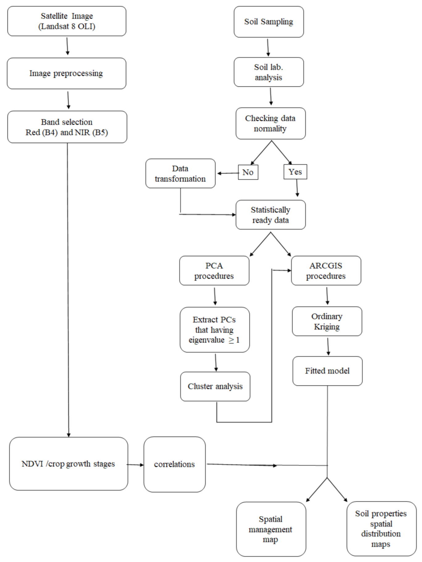
2.3. Remote Sensing and GIS

To monitor the variation of vegetation cover during the crop growth and their correlation with soil salinity, Operational Land Imager (OLI) Path/Row 176/39 with a spatial resolution of 30 m was used during four dates in summer 2019 (June, July, August and stamper). ENVI, 5.1 Software (the Environment for Visualizing Images) was used for image processing and analyses of the OLI satellite data. NDVI was calculated based on the reflectance values in red (visible) and near infrared ranges, where high values of NDVI indicate good soil quality and vice versa. NDVI is formulated as follows:

$$NDVI=\frac{NIR-R}{NIR+R}$$

where NIR represents near-infrared reflectance and R represents visible red reflectance. Four dates of NDVI were determined to track the change of vegetative density, which included the initial growth stage, then vegetative growth, flowering stage, and maturity and harvest stage SPSS were used to analyze the statistical relationship between soil salinity and NDVI. The preprocessing of OLI images was conducted using the FLAASH model according to Felde et al. [48]. Pre-processing of image used in the current study to be checked and corrected the error occurred from different sources such as geometric corrections, filtering and noise removal, and in addition the image resolution was enhanced through sharpening and color balancing [49]. Mapping of soil characteristics was generated using Arc GIS 10.5 where the kriging method was used to interpolate the spatial distribution of soil parameters. During the implementation of semivariogram models of ordinary kriging, soil properties, and their spatial distribution were predicted in unsampled locations of the study area. The fitting models were selected according to values of coefficient determination (R²), root-mean-square error (RMSE) and spatial dependence (SPD). RMSE is defined as the square root of an average squared difference between the observed and predicted values. The SPD was computed using the following equation:

$$RMSE=\sqrt{\frac{SSEi}{n}}$$

where SSE is the sum of errors (observed–estimated values) and n is the number of pairs (errors). The model that has the smallest value of RMSE is considered as the best fitted one. The SPD was computed using the following equation [50]:

$$SPD\left(\%\right)=\frac{\left(c1\right)}{C_0+C_1}\ast 100$$

where C₀ is the nugget effect and C₁ is the contribution. The spatial dependence is weak, moderate and strong when SPD values are <0.25, 0.25 to 0.75 and >0.75, respectively [51]. The outputs of maps are categorized according to the threshold of FAO and USDA.

2.4. Descriptive of Statistics Analysis

The descriptive statistics, including mean, maximum, minimum, standard deviation, kurtosis coefficients, and skewness of data, were computed using the SPSS software version 23. In addition, the normality distribution was examined using the Shapiro–Wilk test at a significance level of α = 0.05. The null hypothesis for this test is that the data are normally distributed. If the chosen alpha level is 0.05 and the p-value is less than 0.05, then the null hypothesis that the data are normally distributed is rejected. If the p-value is greater than 0.05, then the null hypothesis is not rejected. The log-transformation method was used if the data were not normally distributed. The Pearson correlation coefficient (r) test was used to find the association between the characteristics of soil. The r was calculated as shown in the following equation. The correlation coefficient always ranges between −1 to +1 where −1 represents X and Y are negatively correlated and +1 represents X and Y are positively correlated.

$$r=\frac{n(\sum xy)-(\sum x)(\sum y)}{\sqrt{[n\sum x^2-(\sum x^2)][n\sum y^2-(\sum y^2)]}}$$

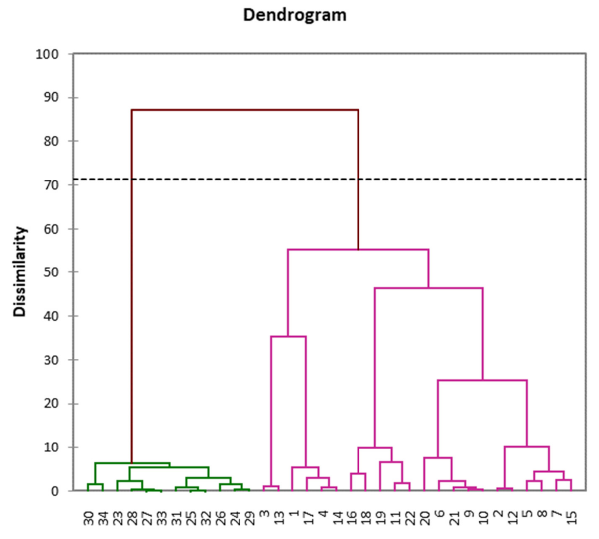
2.5. Principal Component Analysis (PCA) and Cluster Analysis

The principal component analysis is a statistical approach that is used to reduce the number of features in the dataset by identifying the most important principal components (PCs) that explain maximum information about the dataset [34]. SPSS software version 23 was used to preform PCA to reduce the studied variables to new dimension (features) that capture maximum variance (i.e., information) where PCA is a statistical procedure that uses an orthogonal transformation to convert a set of observations of possibly correlated variables into a set of values of linearly uncorrelated variables called principal components “PCs” [52]. PCs having eigenvalues greater than one have been considered whereas PCs less than 1 were neglected [52]. The values of these new variables (PCs) for the observations are called factor scores, and these factors scores can be interpreted geometrically as the projections of the observations onto the principal components [52].

Cluster analysis is a method of gathering a set of soil properties in such a way that properties in the same group (called a cluster) are more similar (in some sense) to each other than to those in other groups (clusters). Ward’s hierarchical clustering method (the proximity type that used was dissimilarity—Euclidean distance) was employed using factor scores instead of the actual dataset to delineate of site-specific management zones. Analysis of variance (Duncan’s test) was used to compare the resultant clusters (zones) from cluster analysis. Finally digital mapping the site-specific management zones was produced by ArcGIS software version 10.5 using ordinary kriging method (see the flowchart in Figure 2).

2.6. Management of Salt Effected Soils

The management of saline soils requires calculating the appropriate gypsum as well as calculating the leaching water to reduce soil salinity to acceptable levels. The gypsum (CaSO₄.2H₂O) requirement (GR) was computed based on the equation of Richards [46] taking into consideration a required final value of exchangeable sodium percent (ESP_f) of 10, and an actual exchangeable sodium percent (ESP_i) initial. The equation is as follows:

$$GR=\frac{ESPi-ESPf}{100}\times CEC\times 1.72$$

where GR is gypsum requirement (cmolc kg⁻¹), ESP_i is initial ESP of the soil (actual ESP of the soil), ESP_f is final ESP of the soil (ESP required to be reached by reclamation), CEC is cation exchange capacity (cmolc kg⁻¹) and 1.72 is the amount (ton) of CaSO₄·2H₂O required to reduce Na⁺ content of the soil by one unit (1 cmolc Na 100 g⁻¹ soil). To convert GR to tons ha⁻¹ it is multiplied by 2.381. The ESP was computed using the following equation:

$$ESP=\frac{Ex. Na}{CEC}\times 100$$

where Ex. Na is the exchangeable sodium expressed as cmolckg⁻¹ soil. The water required for leaching was computed using a simple equation as follows [53].

$$\frac{D_w}{D_s}=\frac{k\times E{C}_{ei}}{E{C}_{ef}}$$

where D_w is the depth of the water required to reduce the initial EC of soil (ECi) in a specific depth of soil profile (Ds) to acceptable EC (final EC “EC_f”) and k is a contestant that equal to 0.45 in organic soil, 0.3 in heavy texture soil or 0.1 in coarse soil. In our study we considered a value of EC_f of 3 and D_s of 0.5 m. To convert D_w to m³ ha⁻¹ it is multiplied by 10,000.

3. Results

3.1. Soil Characteristics

Table 1. Descriptive statistics summary of the studied soil properties.

	Min.	Max.	Mean ± SD	Skewness	Kurtosis	Normality Test *
pH	7.08	8.64	8.03 ± 0.41	−0.68	−0.26	0.074
ECe, dSm−1	5.23	71.92	16.46 ± 14.95	2.91	8.68	<0.0001
SAR	13.36	81.47	39.74 ± 16.68	0.77	−0.13	0.034
CEC, cmolckg−1	21.88	42.25	29.07 ± 5.79	0.74	−0.51	0.001
ESP, %	13.49	44.10	29.73 ± 7.73	0.12	−0.72	0.649
CaCO3, %	1.45	19.31	5.82 ± 4.42	1.52	1.96	<0.0001
Clay, %	33.07	77.64	48.12 ± 11.83	0.91	0.04	0.001
Silt, %	19.38	59.43	39.57 ± 8.49	−0.41	0.90	0.004
Sand, %	2.41	33.93	12.31 ± 7.41	0.53	0.23	<0.0001
BD, Mgm−3	1.10	1.90	1.40 ± 0.18	0.57	0.52	0.69
Porosity, %	28.16	58.77	47.16 ± 6.72	−0.57	0.52	0.69

* Normality test according to Anderson–Darling method.

shows the studied soil properties and its descriptive statistics summary. The results indicated that the pH, ECe, SAR, CEC, ESP and CaCO₃ of the studied soil ranged between 8.03, 16.46 dSm⁻¹, 39.74, 29.07 cmolckg⁻¹, 29.73% and 5.82%, respectively. Concerning soil particles, bulk density and porosity, the values were 48.12% of clay, 39.57% of silt, 12.31% of sand, 1.4 Mgm⁻³ of bulk density, and 47.16% of porosity.

3.2. The Descriptive Statistics Analysis of Soil Properties

According to skewness and kurtosis of the studied soil properties, it is clear that all the studied properties do not subject to a normal distribution except soil pH, ESP, BD and porosity. The results showed the normality test according to the Anderson-Darling method and it was found that p-values were less than 0.05 for all studied soil properties.

The association between the soil properties was illustrated using correlation plot (Figure 3). Correlation plot illustrated that, there was a significant positive correlation for pH with SAR (r = 0.34), CEC (r = 0.43), ESP (r = 0.37) and clay (r = 0.43), on the other hand the correlation was negative with sand (r = −0.65). Regarding the relationship between ECe and other properties, the correlation plot cleared that there was a significant positive correlation with SAR (r = 0.55), CEC (r = 0.48), ESP (r = 0.51) and clay (r = 0.48). Also, there was a significant positive correlation between SAR and ESP (r = 0.97) and a significant negative correlation between SAR and sand (r = −0.40). The correlation of CEC with clay and BD was a significant positive where the r values were 0.99 of clay and 0.35 of BD. On the other hand there was a significant negative correlation between CEC, silt, sand and porosity where the r values were −0.78 of silt, −0.68 of sand and −0.35 of porosity. The association between ESP and sand was a significant negative (r = −0.38). Furthermore. the relationship of clay with silt and sand was a significant negative where the r was −0.38 of silt and −0.38 of sand.

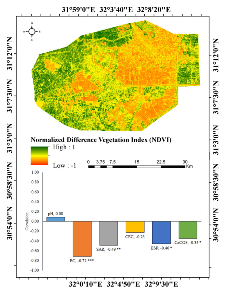
3.3. Normalized Difference Vegetation Index (NDVI)

Figure 4 shows the spatial distribution of NDVI and its relationship with salinity and sodicity indicators. The NDVI values of the study area varied from −0.06 to 0.40. The results showed a highly negatively significant relationship between NDVI with salinity as well as sodicity, where the person correlation coefficient (r) values were −0.72, −0.49, −0.46, −0.35 of soil ECe, SAR, ESP and CaCO₃, respectively. Also, there was no significant correlation between NDVI and CEC (r = −0.23) as well as soil pH (r = 0.08).

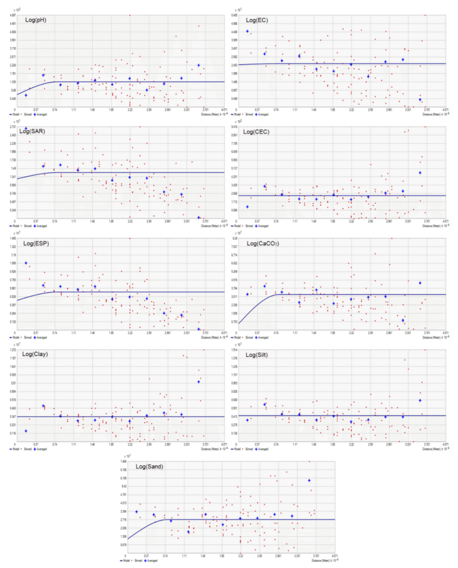
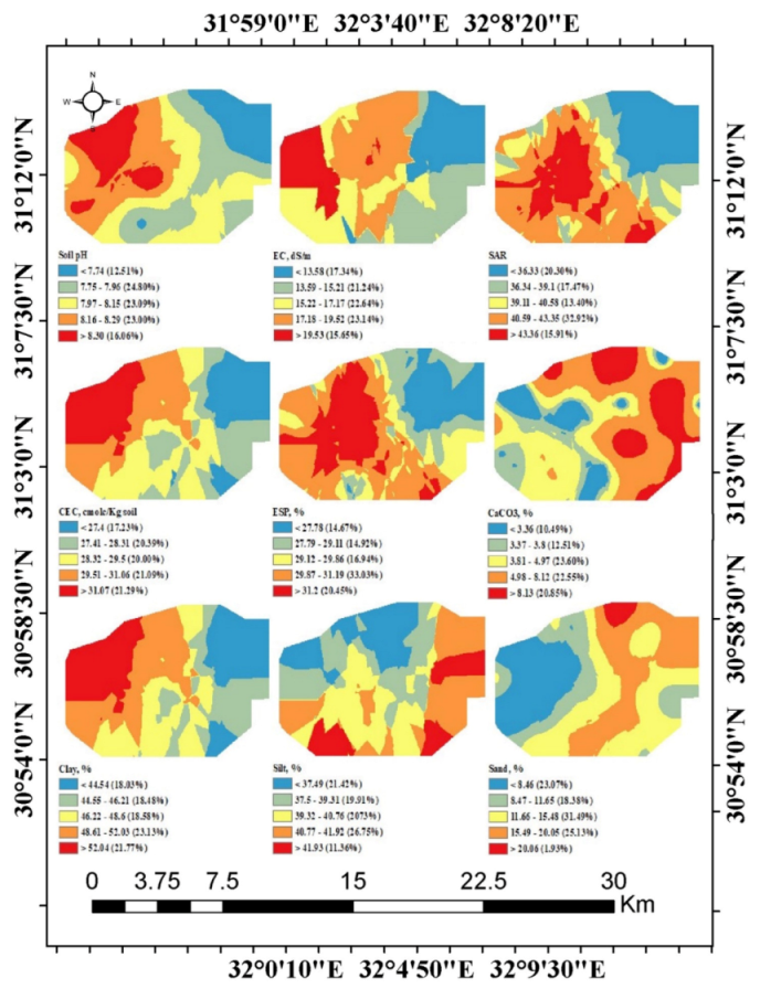
3.4. Spatial Variability of the Studied Soil Properties

The results showed that some of the soil properties did not subject to the normal distribution (Table 1), Therefore the logarithm method used to be transformed before interpolating the spatial distribution of the soil properties using the ordinary kriging method as shown in Figure 5. The results showed that the Gaussian model was the fitting model for a logarithm of soil pH, SAR, CEC, clay, sand and porosity, the pentaspherical model was the fitting model for a logarithm of ECe, ESP and silt, an exponential model was the fitting model for a logarithm of CaCO₃, and a spherical model was the fitting model for a logarithm of BD. The parameters of semi-variogram of all the studied soil properties in study area are listed in

Table 2. Semi-variogram parameter of all the studied soil properties in study area.

Parameters	Model	Nugget	Sill	SPD	Rang	R2	RMSE	Increment	Max. Lag
pH	Gaussian	0.00	0.00	Strong	19,263.8	0.99	0.06	3237.94	14,390.8
ECe	Pentaspherical	0.24	0.35	Moderate	21,656.8	0.36	0.05	3957.48	25,184.0
SAR	Gaussian	0.10	0.07	Weak	55,172.6	0.50	0.03	3237.94	46,770.2
CEC	Gaussian	0.02	0.51	Strong	244,327	0.82	0.00	5756.34	25,184.0
ESP	Pentaspherical	0.05	0.08	Moderate	4887.79	0.67	0.00	2518.4	10,793.1
CaCO3	Exponential	0.16	0.59	Moderate	33,532.7	0.67	0.05	3597.71	25,184.0
Clay	Gaussian	0.02	3.79	Strong	566,998	0.70	0.01	5756.34	39,574.8
Silt	Pentaspherical	0.00	0.06	Strong	5277.02	0.99	0.00	3597.71	7195.42
Sand	Gaussian	0.16	0.69	Strong	26,627.1	0.91	0.05	5396.56	35,977.1
BD	Spherical	0.01	0.02	Moderate	29,692.5	0.97	0.00	4677.02	32,379.4
Porosity	Gaussian	0.01	0.05	Strong	62,815.5	0.72	0.00	3237.94	28,781.7

.

Figure 6 shows the spatial variability maps of the soil properties in the study area. The map of spatial variability of soil pH indicates that the lowest values were less than 7.74 and characterized about 12.51% of the total area, while the highest values were higher than 8.3 and characterized about of 16.6% The rest values of the soil pH ranged between 7.74 to 8.3. The results showed that, ECe greater than 4 dSm⁻¹, this is a reflection of the high salinity condition of the study area (Figure 6). Also, the results showed an increase in SAR values > 13 and ESP values > 15, these high values indicated that, the study area suffers from sodicity. Spatial variability map of CEC showed that 17.23%, 20.39%, 20.00%, 21.09%, and 21.29% of the study area having CEC <27.4, 27.41–28.31, 28.32–29.5, 29.51–31.06, and > 31.07 cmolckg⁻¹, respectively. Also, the spatial variability map of clay, silt and sand indicate that the soil in the study area is clayey. The map showed clearly that 19.08%, 17.54%, 22.72%, 23.04%, and 17.62% of the study area had bulk density <1.36, 41.37–1.39, 1.4–1.41, 1.42–1.44 and >1.45 Mgm⁻³, respectively, and 1.75%, 6.63%, 30.04%, 47.79%, and 13.78% of study area had porosity <40.03%, 40.04–43.22%, 43.23–46.41%, 46.42–49.6%, and >49.61%, respectively.

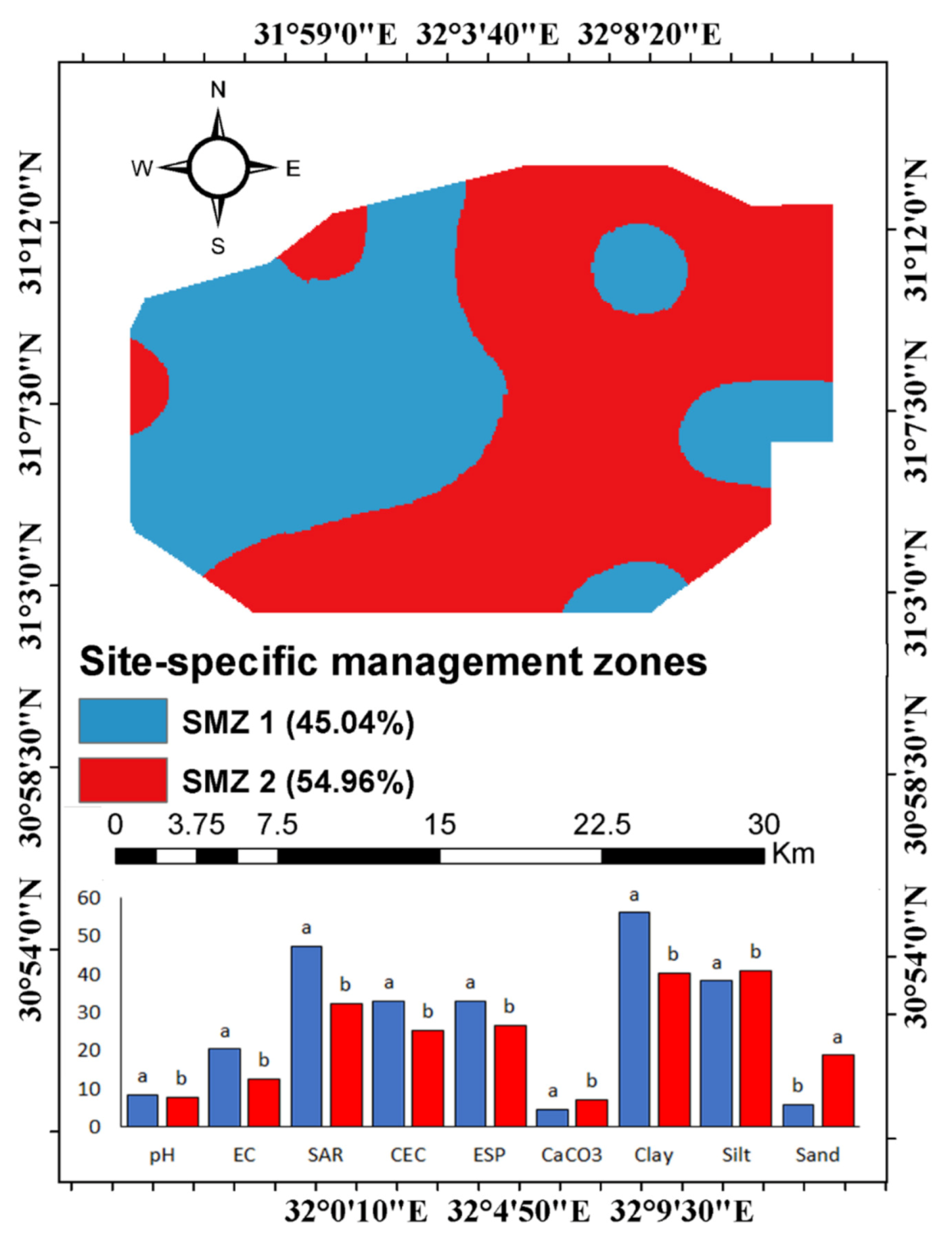
3.5. Spatial Management Zones (SMZ) of Study Area

Table 3. Summary of the principal component analysis (PCA).

	PC1	PC2	PC3	PC4
Eigenvalue	4.39	2.42	1.82	1.23
Variability (%)	39.90	21.98	16.59	11.21
Cumulative %	39.90	61.88	78.47	89.68
* Factor loadings:
pH	0.54	−0.27	0.33	−0.53
EC	0.63	0.04	0.05	0.65
SAR	0.68	0.26	0.61	0.25
CEC	0.90	−0.22	−0.37	−0.05
ESP	0.63	0.25	0.67	0.22
CaCO3	−0.08	0.81	−0.16	0.08
Clay	0.86	−0.36	−0.35	0.00
Silt	−0.57	0.12	0.70	−0.29
Sand	−0.71	0.44	−0.24	0.34
BD	0.48	0.77	−0.19	−0.32
Porosity	−0.48	−0.77	0.19	0.32
PCs scores of observations
1	2.34	−3.36	−2.29	−0.52
2	−0.11	−1.59	0.52	−1.04
3	4.21	−0.98	0.68	2.62
4	0.71	−1.02	−1.17	−1.20
5	0.11	0.03	1.23	−1.63
6	2.44	−0.50	0.99	−0.14
7	−0.49	−1.30	2.81	0.04
8	1.30	0.98	2.45	−0.70
9	2.14	0.84	0.81	−1.22
10	2.70	0.32	0.67	−0.97
11	0.42	0.29	−0.77	0.68
12	−0.21	−1.60	0.00	−1.94
13	4.92	−1.08	−0.65	2.52
14	0.44	−1.78	−1.81	−0.39
15	−1.14	0.75	2.62	−0.56
16	−1.48	3.17	0.19	0.26
17	1.53	−0.51	−3.17	−0.65
18	−1.61	4.09	−2.40	0.91
19	1.13	3.19	−1.60	−1.23
20	3.47	2.46	0.79	0.92
21	1.75	0.84	0.09	−1.63
22	0.37	2.05	−0.23	0.80
23	−1.73	−1.20	1.55	1.68
24	−1.55	0.43	−0.52	−0.59
25	−1.76	−0.68	0.01	−0.57
26	−1.13	0.73	0.63	0.12
27	−2.07	−0.11	0.16	0.56
28	−2.11	−0.57	0.57	1.26
29	−2.06	0.02	−0.60	0.10
30	−3.24	−0.35	−1.65	0.55
31	−2.57	−1.28	−0.13	−0.02
32	−1.67	−0.76	0.52	−0.36
33	−1.93	−0.25	0.04	1.02
34	−3.14	−1.27	−0.37	1.31

* Values in bold correspond for each variable to the factor for which the squared cosine is the largest.

shows the summary of the PCA. The results showed four principal components (PCs) that have eigenvalues greater than 1, so they were considered and the other PCs were neglected. The four PCs explained 89.68% of the studied soil properties’ variability as follows: 39.90%, 21.98%, 16.59% and 11.21% for PC1, PC2, PC3 and PC4, respectively. According to factor loadings, it was clear that soil pH, SAR, CEC and clay were correlated with PC1. On the other hand, calcium carbonate, soil bulk density and porosity were correlated with PC2 while PC3 was correlated with ESP and silt, and PC4 was correlated with EC_e.

According to PCs scores, the cluster analysis showed two dissimilar clusters. The dendrogram of clustering was shown in Figure 7. The statistically significant differences between the two clusters were tested, where the results of the ANOVA (Duncan) test were listed in Table 3. The ANOVA results showed that the first cluster (SMZ1) characterized by average soil properties as follows: pH, ECe, SAR, CEC, ESP, CaCO3, clay, silt sand, BD and porosity were 8.31, 20.32 dSm⁻¹, 47.19, 32.91 cmolckg⁻¹, 32.85%, 4.56%, 55.96%, 38.20%, 5.84%, 1.47 Mgm⁻³, and 44.51%, respectively. On the other hand, the second cluster (SMZ2) was characterized by 7.748, 12.60 dSm⁻¹, 32.30, 25.26 cmolckg⁻1, 26.60%, 7.08%, 40.28%, 40.94%, 18.78%, 1.27 Mgm⁻3, and 52% for pH, ECe, SAR, CEC, ESP, CaCO3, clay, silt sand, BD and porosity, respectively.

Mapping of SMZ was generated using Arc GIS 10.5 where, the kriging method was used to interpolate the spatial distribution of SMZ (Figure 8). The SMZ 1 and SMZ 2 occupied 34,088 hectares (45.04% of study area) and 41,592 hectares (54.96% of study area), respectively (

Table 4. Site specific management zones characteristics.

Parameters	SMZ 1	SMZ 2
pH	8.31 a	7.75 b
EC, dSm−1	20.32 a	12.60 b
SAR	47.19 a	32.30 b
CEC, cmolckg−1	32.91 a	25.23 b
ESP, %	32.85 a	26.60 b
CaCO3, %	4.56 a	7.08 a
Clay, %	55.96 a	40.28 b
Silt, %	38.20 a	40.94 a
Sand, %	5.84 b	18.78 a
Bulk density, Mgm−3	1.47 a	1.270 b
Porosity, %	44.51 b	52.00 a
Area, ha	34,088 (45.04%)	41,592 (54.96%)
GR, cmolckg−1	7.52 (30.8 Mg ha−1)	4.12 (17.15 Mg ha−1)
Dw, m3 ha−1	10,157.56	6300.23

Note: The parameters grouped in the same row and have the same letter mean there is no significance between them according to Duncan multiple range test.

). The amounts of gypsum required to reduce the initial ESP from 32.85% of SMZ 1 and from 26.60% of SMZ 2 to 10% were 7.52 cmolckg⁻¹ (30.8 Mg ha⁻¹) and 4.12 cmolckg⁻¹ (17.15 Mg ha⁻¹), respectively. On the other hand, the amounts of leaching water required to reduce the initial ECe from 20.32 dSm⁻¹ of SMZ 1 and from 12.60 dSm⁻¹ of SMZ 2 to 3 dSm⁻¹ were 10,157.56 m³ ha⁻¹ and 6300.23 m³ ha⁻¹, respectively.

4. Discussion

4.1. Soil Characteristics and Mapping of the Study Area

The alluvial soils located south of lakes in arid and semi-arid conditions suffer from increasing soil degradation processes [54,55]. Soils in the Nile Delta are also exposed to many factors that cause degradation in their chemical and physical properties [7]. The current results reflect soil salinity of the study area ranging between 5.23 to 71.92 dSm⁻¹, this find is consistent with the trend of soil salinity in such conditions dSm⁻¹ [7,26]. However, the highest values of soil salinity reached 71 dSm^−1. The average was 16.46 dSm⁻¹, and this wide range of salinity belongs to management practices and human activities [21]. Furthermore, the subsurface saline groundwater table in the North Nile Delta may cause salinization of those soils especially in the absence of appropriate management practices [7]. In addition, irrigation water may be a source of soil salinization as a result of some farmers undertaking agricultural drainage into irrigation canals [56]. This situation is similar to salt formation in many countries of the Middle East, such as Egypt, Iraq, Saudi Arabia, where the formation of soil salinity is affected by the levels of saline groundwater, which rises by capillary action to the upper surfaces of the soil profile, then forms a thin layer of salts on the surface [57,58]. In such arid conditions, the increase of salt concentration in the root soon leads to osmotic stress and limits the absorption of water and nutrients from the soil, and also may lead to inducing toxicity within the plant cells [59].

According to the FAO [60] the soils of the study area are classified saline-sodic where it has high values of SAR and ESP. The average values of both of SAR and ESP are 39.74 and 29.73, respectively. These results indicated that the study area is exposed to chemical degradation. The increase of sodicity levels has adverse impacts on soil and leads to degradation in their chemical properties such as damage of the soil structure and their aggregation, therefore affecting the availability of nutrition, crop growth, and yield production [61,62]. The correlation between salinity and other soil properties confirms that the soils of the study area are classified as saline or saline-alkali with the predominance of sodium cation and chloride anion, this explains the positive correlation between EC and SAR, ESP, and CEC, where (r was 0.55, 0.51, 0.48, respectively). These results are consistent with the studies conducted in the soil located south of the lakes in the north Nile Delta [7,63,64]. On the other hand, there are negative correlations between porosity and clay, CEC, Silt sand these results reflected that the area is exposed to soil compaction due to mismanagement [7].

Figure 4 and Figure 5 show the spatial distribution using Kriging methods of soil characteristics of the study area. The selected suitable model among semi-variogram models is based on R² and RMSE. The results presented in Table 2 indicate that R² varied from 0.5 to 0.99. In addition, the values of RMSE ranged from 0.0 to 1.06, they are close to zero for all maps of soil characteristics. These results confirmed that the selected models were the best among semi variogram models to map the spatial variation of the soil characteristics in the current study and are consistent with [65].

Crop health is a good indicator for soil quality [24], where, the development of crop growth is associated with the soil physical and chemical properties [66]. NDVI values indicated vegetation health, soil quality, and management practices [67]. The comparison of soil salinity with the average density of vegetation during the summer season showed a good correlation. Figure 3 shows that, the main NDVI values in the study area ranged between −0.06 to 0.4. These average values of NDVI are nearly low comparing the other irrigated areas in Nile Delta [26]. Furthermore, Pearson’s correlation test showed a logical negative correlation (r = −0.72) between salinity and the NDVI index, and this confirms that soil salinity effectively impacts on crop growth [68]. Hence, NDVI is a good indicator as it is characterized by the spectral responses of bio-mass, which is a function of the spatial variation in soil quality degrees and its harmony and correlation with health, the density of vegetation cover, and soil productivity [24].

4.2. Mapping and Analyses of the Spatial Management Zones

PCA was used in many studies of soil to analyze and classify their characteristics [69]. The results showed that the soil properties were classified into four PCs that have eigenvalues bigger than 1 and that explain 89.68% of the total variables. The first PC gathers the soil properties that are associated together in one cluster, where the salt-affected soils in the Nile Delta are characterized by rising pH, SAR, CEC, and clay in the same direction [7,13]. The second PC2 cluster includes those soil characteristics that interact with each other in negative relationships where PC2 included calcium carbonate, soil bulk density, and porosity that have negatively correlated with each other, and this is consistent with [70,71].

The results showed that the soils of the study area were classified into two management zones using a dendrogram cluster (Figure 6). Based on the homogeneity in their properties, the soils were grouped into two clusters. The results showed that, p-value < 0.05, and this confirm that there is a significant statistical difference between the two clusters. The average values of soil properties in both classes reflect the existing situation of agricultural practice in the north of the Nile Delta [64].

The map of SMZ (Figure 7) provides an illustration, about the spatial distribution of the agricultural management practices of both classes in the study area. Both SMZ classes suffer from increasing EC, SAR and ESP where the averages are larger than the threshold values [46]. Furthermore, SMZ1 has average values of bulk density reached to 1.47 Mgm⁻³ this means that, the area is exposed the compaction due to mismanagement, these findings agree with [7,64]. Therefore, the suggested recommendation of agricultural management in the study area may be linked the requirements to decrease EC, SAR and ESP with the spatial location. The quantities of excess water for salt leaching were calculated according to the concentration of salts in the soil profile and the physical properties according to Gupta [53]. Also, the proposed quantities of gypsum for correction of soil sodicity of saline sodic were calculated according Richards [46]. The organic additions to saline and sodicity soils are important as they lead to many benefits such as improving the physical properties, affecting the activity of microorganisms and improving the soil texture and structure [54]. Moreover, the application of proper tillage of the soil is also important in improving the properties of the soil [64].

5. Conclusions

The integration between PCA and GIS provides unconventional solutions to assess the spatial dimension of soil salinization and their distribution which is considered the first step towards the effective management practices. The results reflected that the soils of the northern Nile Delta suffer from active salinization processing. Using PCA and GIS, the soil of the study area could be classified into two management zones based on the chemical and physical properties.

The PCA results showed that the first four PCs could be explained by 89.6% of the total variability in the soil properties. Furthermore, the variance analysis results showed that most of the soil attributes and biomass presented statistical differences in each management zone.

Moreover, the classification of the area into zones could facilitate management procedures. The NDVI indicator was necessary for following up on the condition of the soils as a guide to soil quality in salt-affected soils. The study recommends adding about 30.8 Mg ha⁻¹ of gypsum in the first zone (SMZ 1) and about 17.15 Mg ha⁻¹ for the second zone (SMZ2) to improve the soils’ physical and chemical properties in the study area.

On the other hand, the first zone needs about 10,157 m³ ha⁻¹ of leaching water to reduce the salinity from 20.32 dSm⁻¹ to the acceptable levels and the second zone needs about 6300 m³ ha⁻¹ to reduce the ECe from 12.60 dSm⁻¹ to 3 dSm⁻¹ in the SMZ 2.

References

1. Lyu, S.; Chen, W.; Zhang, W.; Fan, Y.; Jiao, W. Wastewater reclamation and reuse in China: Opportunities and challenges. J. Environ. Sci. 2016, 39, 86–96. [Google Scholar] [CrossRef] [PubMed]
2. El Baroudy, A.A. Geomatics-based soil mapping and degradation risk assessment of Nile delta soils. Pol. J. Environ. Stud. 2010, 1123, 1131. [Google Scholar]
3. Shokr, M.S.; Abdellatif, M.; El Baroudy, A.A.; Elnashar, A.; Ali, E.F.; Belal, A.A.; Attia, W.; Ahmed, M.; Aldosari, A.A.; Szantoi, Z. Development of a spatial model for soil quality assessment under arid and semi-arid conditions. Sustainability 2021, 13, 2893. [Google Scholar] [CrossRef]
4. El Nahry, A.; Ibraheim, M.; El Baroudy, A. Assessment of soil degradation in the northern part of Nile Delta, Egypt, using remote sensing and GIS techniques. Egypt. J. Remote Sens. Space Sci. 2008, 11, 139–154. [Google Scholar]
5. Hassan, A.; Belal, A.; Hassan, M.; Farag, F.; Mohamed, E. Potential of thermal remote sensing techniques in monitoring waterlogged area based on surface soil moisture retrieval. J. Afr. Earth Sci. 2019, 155, 64–74. [Google Scholar] [CrossRef]
6. Hendawy, E.; Belal, A.; Mohamed, E.; Elfadaly, A.; Murgante, B.; Aldosari, A.A.; Lasaponara, R. The prediction and assessment of the impacts of soil sealing on agricultural land in the North Nile Delta (Egypt) using satellite data and GIS modeling. Sustainability 2019, 11, 4662. [Google Scholar] [CrossRef] [Green Version]
7. Mohamed, E.; Schütt, B.; Belal, A. Assessment of environmental hazards in the north western coast-Egypt using RS and GIS. Egypt. J. Remote Sens. Space Sci. 2013, 16, 219–229. [Google Scholar] [CrossRef] [Green Version]
8. Mohamed, E.S.; Belal, A.; Shalaby, A. Impacts of soil sealing on potential agriculture in Egypt using remote sensing and GIS techniques. Eurasian Soil Sci. 2015, 48, 1159–1169. [Google Scholar] [CrossRef]
9. Mohamed, E.S.; Saleh, A.; Belal, A. Sustainability indicators for agricultural land use based on GIS spatial modeling in North of Sinai-Egypt. Egypt. J. Remote Sens. Space Sci. 2014, 17, 1–15. [Google Scholar] [CrossRef] [Green Version]
10. FAO. Global Network on Integrated Soil Management for Sustainable Use of Salt-Affected Soils; FAO Land and Plant Nutrition Management Service: Rome, Italy, 2005; pp. 12–19. [Google Scholar]
11. Pitman, M.G.; Läuchli, A. Global impact of salinity and agricultural ecosystems. In Salinity: Environment-Plants-Molecules; Springer: Berlin/Heidelberg, Germany, 2002; pp. 3–20. [Google Scholar]
12. Mohamed, E.S.; Belal, A.; Saleh, A. Assessment of land degradation east of the Nile Delta, Egypt using remote sensing and GIS techniques. Arab. J. Geosci. 2013, 6, 2843–2853. [Google Scholar] [CrossRef]
13. AbdelRahman, M.A.; Shalaby, A.; Mohamed, E. Comparison of two soil quality indices using two methods based on geographic information system. Egypt. J. Remote Sens. Space Sci. 2019, 22, 127–136. [Google Scholar] [CrossRef]
14. Said, M.E.S.; Ali, A.; Borin, M.; Abd-Elmabod, S.K.; Aldosari, A.A.; Khalil, M.; Abdel-Fattah, M.K. On the use of multivariate analysis and land evaluation for potential agricultural development of the northwestern coast of Egypt. Agronomy 2020, 10, 1318. [Google Scholar] [CrossRef]
15. Sharma, D.K.; Singh, A. Current trends and emerging challenges in sustainable management of salt-affected soils: A critical appraisal. In Bioremediation of Salt Affected Soils: An Indian Perspective; Springer: Berlin/Heidelberg, Germany, 2017; pp. 1–40. [Google Scholar]
16. Zörb, C.; Geilfus, C.M.; Dietz, K.J. Salinity and crop yield. Plant Biol. 2019, 21, 31–38. [Google Scholar] [CrossRef]
17. Daliakopoulos, I.; Tsanis, I.; Koutroulis, A.; Kourgialas, N.; Varouchakis, A.; Karatzas, G.; Ritsema, C. The threat of soil salinity: A European scale review. Sci. Total Environ. 2016, 573, 727–739. [Google Scholar] [CrossRef]
18. Aldabaa, A.A.A.; Weindorf, D.C.; Chakraborty, S.; Sharma, A.; Li, B. Combination of proximal and remote sensing methods for rapid soil salinity quantification. Geoderma 2015, 239, 34–46. [Google Scholar] [CrossRef] [Green Version]
19. Abd-Elmabod, S.K.; Mansour, H.; Hussein, A.; Mohamed, E.; Zhang, Z.; Anaya-Romero, M.; Jordán, A. Influence of irrigation water quantity on the land capability classification. Plant Arch. 2019, 2, 2253–2561. [Google Scholar]
20. Hegab, I. Restrictions of Bordering Idko Lake Low Soil Productivity, North Nile Delta. J. Soil Sci. Agric. Eng. 2014, 5, 157–167. [Google Scholar] [CrossRef]
21. Mohamed, E.S.; Abu-hashim, M.; AbdelRahman, M.A.; Schütt, B.; Lasaponara, R. Evaluating the effects of human activity over the last decades on the soil organic carbon pool using satellite imagery and GIS techniques in the Nile Delta Area, Egypt. Sustainability 2019, 11, 2644. [Google Scholar] [CrossRef] [Green Version]
22. Seifi, M.; Ahmadi, A.; Neyshabouri, M.-R.; Taghizadeh-Mehrjardi, R.; Bahrami, H.-A. Remote and Vis-NIR spectra sensing potential for soil salinization estimation in the eastern coast of Urmia hyper saline lake, Iran. Remote Sens. Appl. Soc. Environ. 2020, 20, 100398. [Google Scholar] [CrossRef]
23. Pettorelli, N. The Normalized Difference Vegetation Index; Oxford University Press: Oxford, UK, 2013. [Google Scholar]
24. Baroudy, A.A.E.; Ali, A.; Mohamed, E.S.; Moghanm, F.S.; Shokr, M.S.; Savin, I.; Poddubsky, A.; Ding, Z.; Kheir, A.; Aldosari, A.A. Modeling land suitability for rice crop using remote sensing and soil quality indicators: The case study of the nile delta. Sustainability 2020, 12, 9653. [Google Scholar] [CrossRef]
25. Mohamed, E.S.; Baroudy, A.; El-beshbeshy, T.; Emam, M.; Belal, A.; Elfadaly, A.; Aldosari, A.A.; Ali, A.; Lasaponara, R. Vis-NIR Spectroscopy and Satellite Landsat-8 OLI Data to Map Soil Nutrients in Arid Conditions: A Case Study of the Northwest Coast of Egypt. Remote Sens. 2020, 12, 3716. [Google Scholar] [CrossRef]
26. Hammam, A.; Mohamed, E. Mapping soil salinity in the East Nile Delta using several methodological approaches of salinity assessment. Egypt. J. Remote Sens. Space Sci. 2020, 23, 125–131. [Google Scholar] [CrossRef]
27. Hufkens, K.; Melaas, E.K.; Mann, M.L.; Foster, T.; Ceballos, F.; Robles, M.; Kramer, B. Monitoring crop phenology using a smartphone based near-surface remote sensing approach. Agric. For. Meteorol. 2019, 265, 327–337. [Google Scholar] [CrossRef]
28. Saleh, A.; Belal, A.; Mohamed, E. Land resources assessment of El-Galaba basin, South Egypt for the potentiality of agriculture expansion using remote sensing and GIS techniques. Egypt. J. Remote Sens. Space Sci. 2015, 18, S19–S30. [Google Scholar] [CrossRef] [Green Version]
29. Gavioli, A.; de Souza, E.G.; Bazzi, C.L.; Guedes, L.P.C.; Schenatto, K. Optimization of management zone delineation by using spatial principal components. Comput. Electron. Agric. 2016, 127, 302–310. [Google Scholar] [CrossRef]
30. Liu, W.; Lu, F.; Chen, G.; Xu, X.; Yu, H. Site-specific management zones based on geostatistical and fuzzy clustering approach in a coastal reclaimed area of abandoned salt pan. Chil. J. Agric. Res. 2021, 81, 420–433. [Google Scholar] [CrossRef]
31. Fridgen, J.J.; Kitchen, N.R.; Sudduth, K.A.; Drummond, S.T.; Wiebold, W.J.; Fraisse, C.W. Management Zone Analyst (MZA) Software for Subfield Management Zone Delineation. Agron. J. 2004, 96, 100–108. [Google Scholar]
32. Moharana, P.; Jena, R.; Pradhan, U.; Nogiya, M.; Tailor, B.; Singh, R.; Singh, S. Geostatistical and fuzzy clustering approach for delineation of site-specific management zones and yield-limiting factors in irrigated hot arid environment of India. Precis. Agric. 2020, 21, 426–448. [Google Scholar] [CrossRef]
33. John, K.; Afu, S.; Isong, I.; Aki, E.; Kebonye, N.; Ayito, E.; Chapman, P.; Eyong, M.; Penížek, V. Mapping soil properties with soil-environmental covariates using geostatistics and multivariate statistics. Int. J. Environ. Sci. Technol. 2021, 18, 3327–3342. [Google Scholar] [CrossRef]
34. Jolliffe, I.T.; Cadima, J. Principal component analysis: A review and recent developments. Philos. Trans. R. Soc. A Math. Phys. Eng. Sci. 2016, 374, 20150202. [Google Scholar] [CrossRef]
35. Perez, L.V. Principal Component Analysis to Address Multicollinearity; Whitman College: Walla Walla, WA, USA, 2017. [Google Scholar]
36. Dandpat, S.K.; Meher, S. Performance improvement for face recognition using PCA and two-dimensional PCA. In Proceedings of the 2013 International Conference on Computer Communication and Informatics, Coimbatore, India, 4–6 January 2013; pp. 1–5. [Google Scholar]
37. Ilin, A.; Raiko, T. Practical approaches to principal component analysis in the presence of missing values. J. Mach. Learn. Res. 2010, 11, 1957–2000. [Google Scholar]
38. Müller, W.; Nocke, T.; Schumann, H. Enhancing the visualization process with principal component analysis to support the exploration of trends. In Proceedings of the 2006 Asia-Pacific Symposium on Information Visualisation, Tokyo, Japan, 1–3 February 2006; Volume 60, pp. 121–130. [Google Scholar]
39. Ivosev, G.; Burton, L.; Bonner, R. Dimensionality reduction and visualization in principal component analysis. Anal. Chem. 2008, 80, 4933–4944. [Google Scholar] [CrossRef] [PubMed] [Green Version]
40. Li, Y.; Shi, Z.; Li, F.; Li, H.-Y. Delineation of site-specific management zones using fuzzy clustering analysis in a coastal saline land. Comput. Electron. Agric. 2007, 56, 174–186. [Google Scholar] [CrossRef]
41. Peralta, N.R.; Costa, J.L.; Balzarini, M.; Angelini, H. Delineation of management zones with measurements of soil apparent electrical conductivity in the southeastern pampas. Can. J. Soil Sci. 2013, 93, 205–218. [Google Scholar] [CrossRef]
42. Molin, J.P.; Castro, C.N.d. Establishing management zones using soil electrical conductivity and other soil properties by the fuzzy clustering technique. Sci. Agric. 2008, 65, 567–573. [Google Scholar] [CrossRef] [Green Version]
43. Metwally, M.S.; Shaddad, S.M.; Liu, M.; Yao, R.-J.; Abdo, A.I.; Li, P.; Jiao, J.; Chen, X. Soil properties spatial variability and delineation of site-specific management zones based on soil fertility using fuzzy clustering in a hilly field in Jianyang, Sichuan, China. Sustainability 2019, 11, 7084. [Google Scholar] [CrossRef] [Green Version]
44. Taxonomy, S. Key to Soil Taxonomy; United States Department of Agriculture, Natural Resources Conservation Service: Washington, DC, USA, 2010. [Google Scholar]
45. EI-Fayoumy, I.F. Geology of Ground Water Supplies in the Region East of the Nile Delta. Ph.D. Thesis, Faculty of Science, Cairo University, Cairo, Egypt, 1968. [Google Scholar]
46. Richards, L.A. Diagnosis and Improvement of Saline and Alkali Soils; LWW: Philadelphia, PA, USA, 1954; Volume 78. [Google Scholar]
47. Van, R.L. Procedures for soil analysis. In International Soil Reference and Information Centre (ISRIC), Food and Agriculture Organization of the United Nations, 6th ed.; Food and Agriculture Organization of the United Nations: Wageningen, The Netherlands, 2002. [Google Scholar]
48. Felde, G.W.; Anderson, G.P.; Cooley, T.W.; Matthew, M.W.; Berk, A.; Lee, J. Analysis of Hyperion data with the FLAASH atmospheric correction algorithm. In Proceedings of the 2003 IEEE International Geoscience and Remote Sensing Symposium, Toulouse, France, 21–25 July 2003; pp. 90–92. [Google Scholar]
49. Zanter, K. Landsat 8 (L8) Data Users Handbook (Version 2.0); USGS: Reston, VA, USA, 2016. [Google Scholar]
50. Biondi, F.; Myers, D.E.; Avery, C.C. Geostatistically modeling stem size and increment in an old-growth forest. Can. J. For. Res. 1994, 24, 1354–1368. [Google Scholar] [CrossRef]
51. Cambardella, C.; Elliott, E. Carbon and nitrogen dynamics of soil organic matter fractions from cultivated grassland soils. Soil Sci. Soc. Am. J. 1994, 58, 123–130. [Google Scholar] [CrossRef]
52. Abdi, H.; Williams, L.J. Principal component analysis. Wiley Interdiscip. Rev. Comput. Stat. 2010, 2, 433–459. [Google Scholar] [CrossRef]
53. Gupta, S.K. Drainage Engineering: Principles and Practices; Scientific Publishers: Singapore, 2019. [Google Scholar]
54. Abu-Hashim, M.; Mohamed, E.; Belal, A.-E. Identification of potential soil water retention using hydric numerical model at arid regions by land-use changes. Int. Soil Water Conserv. Res. 2015, 3, 305–315. [Google Scholar] [CrossRef] [Green Version]
55. El Nahry, A.; Mohamed, E. Potentiality of land and water resources in African Sahara: A case study of south Egypt. Environ. Earth Sci. 2011, 63, 1263–1275. [Google Scholar] [CrossRef]
56. Abdel-Fattah, M.K.; Abd-Elmabod, S.K.; Aldosari, A.A.; Elrys, A.S.; Mohamed, E.S. Multivariate analysis for assessing irrigation water quality: A case study of the Bahr Mouise Canal, Eastern Nile Delta. Water 2020, 12, 2537. [Google Scholar] [CrossRef]
57. Qureshi, A.S.; Al-Falahi, A.A. Extent, characterization and causes of soil salinity in central and southern Iraq and possible reclamation strategies. Int. J. Eng. Res. Appl. 2015, 5, 84–94. [Google Scholar]
58. Al-Wabel, M.I.; Sallam, A.; Ahmad, M.; Elanazi, K.; Usman, A.R. Extent of climate change in Saudi Arabia and its impacts on agriculture: A case study from Qassim region. In Environment, Climate, Plant and Vegetation Growth; Springer: Berlin/Heidelberg, Germany, 2020; pp. 635–657. [Google Scholar]
59. Youssef, A.M. Salt tolerance mechanisms in some halophytes from Saudi Arabia and Egypt. Res. J. Agric. Biol. Sci. 2009, 5, 191–206. [Google Scholar]
60. FAO. Land Quality Indicators and Their Use in Sustainable Agriculture and Rural Development. In Land and Water Bulletin 5; FAO: Rome, Italy, 1997. [Google Scholar]
61. Nan, J.; Chen, X.; Chen, C.; Lashari, M.S.; Deng, J.; Du, Z. Impact of flue gas desulfurization gypsum and lignite humic acid application on soil organic matter and physical properties of a saline-sodic farmland soil in Eastern China. J. Soils Sediments 2016, 16, 2175–2185. [Google Scholar] [CrossRef]
62. Gonçalo Filho, F.; da Silva Dias, N.; Suddarth, S.R.P.; Ferreira, J.F.; Anderson, R.G.; dos Santos Fernandes, C.; de Lira, R.B.; Neto, M.F.; Cosme, C.R. Reclaiming tropical saline-sodic soils with gypsum and cow manure. Water 2020, 12, 57. [Google Scholar] [CrossRef] [Green Version]
63. El Behairy, R.A.; El Baroudy, A.; Ibrahim, M.; Shokr, M. Assessment and mapping of surface water quality index for irrigation purpose: Case study northwest of Nile Delta, Egypt. Menoufia J. Soil Sci. 2021, 6, 163–182. [Google Scholar] [CrossRef]
64. Deshesh, T. Amelioration of salt affected soils and its productivity using soil amendments and tillage System. Menoufia J. Soil Sci. 2021, 6, 31–47. [Google Scholar] [CrossRef]
65. Johnston, K.; Ver Hoef, J.M.; Krivoruchko, K.; Lucas, N. Using ArcGIS Geostatistical Analyst; Esri Redlands: New York, NY, USA, 2001; Volume 380. [Google Scholar]
66. Abdel-Fattah, M.K.; Mohamed, E.S.; Wagdi, E.M.; Shahin, S.A.; Aldosari, A.A.; Lasaponara, R.; Alnaimy, M.A. Quantitative evaluation of soil quality using Principal Component Analysis: The case study of El-Fayoum depression Egypt. Sustainability 2021, 13, 1824. [Google Scholar] [CrossRef]
67. Jiapaer, G.; Chen, X.; Bao, A. A comparison of methods for estimating fractional vegetation cover in arid regions. Agric. For. Meteorol. 2011, 151, 1698–1710. [Google Scholar] [CrossRef]
68. Machado, R.M.A.; Serralheiro, R.P. Soil salinity: Effect on vegetable crop growth. Management practices to prevent and mitigate soil salinization. Horticulturae 2017, 3, 30. [Google Scholar] [CrossRef]
69. Choudhury, B.U.; Mandal, S. Indexing soil properties through constructing minimum datasets for soil quality assessment of surface and profile soils of intermontane valley (Barak, North East India). Ecol. Indic. 2021, 123, 107369. [Google Scholar] [CrossRef]
70. Chaudhari, P.R.; Ahire, D.V.; Ahire, V.D.; Chkravarty, M.; Maity, S. Soil bulk density as related to soil texture, organic matter content and available total nutrients of Coimbatore soil. Int. J. Sci. Res. Publ. 2013, 3, 1–8. [Google Scholar]
71. Gothwal, R.; Jangir, O. Assessment of soil properties of a lentic ecosystem in semiarid region: Nakki Lake, Mount Abu, India. World Sci. News 2020, 149, 81–91. [Google Scholar]
Figure 1. Location of the study area.
Agronomy 11 02510 g001
Figure 2. Framework of methodology used in this study.
Agronomy 11 02510 g002
Figure 3. Correlation plot of the studied soil properties.
Agronomy 11 02510 g003
Figure 4. Digital mapping of the Normalized Difference Vegetation Index (NDVI) and its association with studied soil properties. *, ** and *** the stars indicate the significant degrees between the NDVI and soil properties.
Agronomy 11 02510 g004
Figure 5. Semi-variogram of models of the different studied soil properties.
Agronomy 11 02510 g005
Figure 6. Spatial variability maps of the studied soil properties in study area.
Agronomy 11 02510 g006
Figure 7. Dendrogram of agglomerative hierarchical clustering (AHC).
Agronomy 11 02510 g007
Figure 8. Digital mapping of the studied soil properties. The parameters grouped in the same row and have the same letter mean there is no significance between them according to Duncan’s multiple range test.
Agronomy 11 02510 g008