1. Introduction
According to the United Nations Organization for Food and Agriculture Organization (FAO) pesticides are any substance, or mixture of substances of chemical or biological ingredients, which are meant for repelling, destroying, or controlling any pest, or regulating plant growth [
1]. These agents play a crucial role in reducing crop losses due to weed/pest infestation and increasing crop yield and quality [
2].
However, pesticide occurrence is threatening surface water and groundwater at global scale [
3,
4,
5,
6] and, besides potentially causing environmental damage and having health implications [
7], may cause prohibition of water use or high treatment costs, especially when associated with drinking water [
8,
9,
10].
Pesticide usage is then one of the cases where the balance between agronomic production sustainability and ecosystem service protection (i.e., water supply) is a very a fragile one. This holds especially true for the groundwater resources that, once contaminated, are very difficult to remediate.
Notwithstanding its importance, the vulnerability of groundwater systems to pesticide has not often been addressed. The concept of aquifer vulnerability refers to the possibility of contaminants percolating through the unsaturated zone to the groundwater. While the vulnerability assessment only refers to the physical factors that may favor, or not, transport processes of substances to the groundwater table; this is often referred as aquifer sensitivity, natural vulnerability, or intrinsic vulnerability [
11]. We refer in contrast to specific vulnerability, when the vulnerability assessment exercise includes the physical-chemical properties of the potential pollutant. A spatially defined aquifer vulnerability assessment to pesticide is important because it may allow outlining agricultural areas where certain compounds should be used following well-defined agronomic practices and/or limitations.
Several methods have been developed to assess both intrinsic and specific aquifer vulnerability; comprehensive reviews on the subject may be found, i.e., in [
12,
13,
14]. Liang et al. (2019) [
15] divided the methods to compute aquifer vulnerability roughly into three types: statistical, process-based, and index-overlay. According to these authors, the index-overlay method is the most widely used method, mainly because of its simplicity, lower data requirement, and clarity in description of vulnerability. In fact, most of the published examples of assessments of groundwater vulnerability to pesticide are based on index-overlay methods performed using Geographic Information System (GIS) desktop applications, modified from methods to evaluate intrinsic vulnerability. The emergence and rapid diffusion of GIS during the last 20 years facilitated the assessment of groundwater vulnerability through mapping, even since its first appearance [
16]. However, a search at hand run on the SCOPUS database for the years 2000/2020 using the words
pesticide and
groundwater and
vulnerability found only 31 relevant records, with slowly increasing interest in the topic since 2015. Among these, Saha & Alam (2014) [
17] estimated vulnerability to pesticide using a modified version of the DRASTIC model (probably the best-known method for assessing aquifer intrinsic vulnerability at global scale [
18]), the pesticide DRASTIC, which was applied to an intense agricultural area of the Gangetic plains in India. Bartzas et al. (2015) [
19] evaluated the pesticide DRASTIC and susceptibility index (SI) methods within a GIS framework, to assess groundwater vulnerability in the agricultural area of Albenga (northern Italy). The results indicated “high” to “very high” vulnerability to groundwater contamination along the coastline and the middle part of the Albenga plain, for almost 49% and 56% of the total study area for the two methods, respectively. Still in India, Duttagupta et al. (2020) [
20] made a first attempt to evaluate the groundwater vulnerability to insecticides and herbicides pollution due to anthropogenic activities across the Western Bengal basin using an index-overlay method. They found that the area under investigation is highly susceptible to pesticide pollution. Douglas et al. (2018) [
21] evaluated the ability of intrinsic (DRASTIC) and specific (attenuation factor; AF) vulnerability models to define groundwater vulnerability areas by comparing model results to the presence of pesticides from groundwater sample datasets. They found that, compared to the DRASTIC model, the AF model more accurately predicted the distribution of the number of contaminated wells within each vulnerability class.
All the above-mentioned methods require many parameters. Schlosser et al. (2002) [
22] developed a simplified method to assess aquifer vulnerability to pesticide contamination at sub-regional scale incorporating relevant hydrologic and pesticide transport parameters. In this study, after introducing the vulnerability index (VI) model [
22], we present and discuss an application to the agricultural area of the Municipality of San Giuliano Terme (Pisa, Italy) in order to focus on the data needs and discuss the reliability of this method (as an example of index-overlay methods).
2. Material and Methods
2.1. The Vulnerability Index Model
The vulnerability index (VI) model is based on the steady state advective transport of the pesticides through the vadose zone, including sorption and degradation processes. It is a modified version of the leaching potential index vulnerability model [
23].
The VI method defines a vulnerability index, for a given area of land, derived from the following relationship:
where: K is the saturated hydraulic conductivity in the porous medium [L/T]; θ
FC is the water content at field capacity [L
3/L
3]; z is the thickness of the considered soil layer [L]; ρ
b is the bulk density [M/L
3]; (%OM) is the percent organic matter content in the soil (in %, dimensionless); t
1/2 is the half life time [T]; K
OC is the pesticide organic-carbon partitioning coefficient [L
3/M]; F
DGW is a factor to account for the depth to water table (dimensionless). The index obtained for an area is assigned to one of the vulnerability classes according to the values reported in
Table 1.
The authors [
22] successfully validated the method by comparing the identified vulnerability classes with analytical results on the presence (or not) of active ingredients (AI) in groundwater.
2.2. The Case Study Area
The San Giuliano Terme agricultural area is located few kms north-west of Pisa and it is part of the Pisa plain, in central-western Tuscany, along the Ligurian coast (
Figure 1).
In 2011, we surveyed a total of 25 farms using the methodology presented in Silvestri et al. (2012) [
24] in the plain area of the San Giuliano Terme municipality covering 2175 ha of utilized agricultural area (UAA), including about 20% of the farms in the area, and about 50% of the UAA (ARTEA, 2010) [
25]. Among the farms surveyed, cereal-industrial cropping systems prevailed, even if there were small areas where vegetable and woody crop cultivation was dominant. The two most widespread crops (
Table 2) in the surveyed area were durum wheat (29.9%) and corn (23.4% of the UAA), followed by sunflower (11.9%) and rapeseed (9.7%). Tomatoes (2.4%) prevailed among vegetables, and olive trees (2.1%) and alfalfa (1.8%) among woody and fodder crops, respectively.
Data on AI use were retrieved by interviewing farmers. We identified 33 different AIs used in the area (
Table 3). Herbicides were the most used pesticides (31 AIs), while only two pesticides were used to control insects (flonicamid) or cryptogams (ziram) (
Table 3).
The large use of herbicide to weeding of the agricultural areas was justified by the above-mentioned predominance of commodities (cereals and industrial crops) and by the consequent limited spread of vegetables and fruits, which usually require a large use of insecticides and fungicides.
About the average amount of spraying, the acetochlor displayed the largest dose (4200 g/ha), followed by glyphosate, MCPA (2-methyl-4-chlorophenoxyacetic acid), metazachlor, s-metolachlor, and ziram (all around 1000 g/ha). The doses of the other AIs were generally lower, in 14 out 33 cases under 100 g/ha. Oxadiazon (t1/2 = 502 gg), lenacil (t1/2 = 179 gg) and aclonifen (t1/2 = 117 gg) are the compounds with longer half-life time. All the other active ingredients show half-life time lower than 100 days and 12 molecules lower than 10 days.
Figure 2 shows the soil map [
26] for the investigated area. Three main types of soil (FAB1, GRE1, and STS1;
Table 4) occupy most of the area of interest. The plain hosts many water-wells with depths varying from a few meters to nearly 250 m, which tap a multilayered confined aquifer made up of Pleistocene sands and gravels [
27]. In the shallowest levels, unconfined aquifers are present [
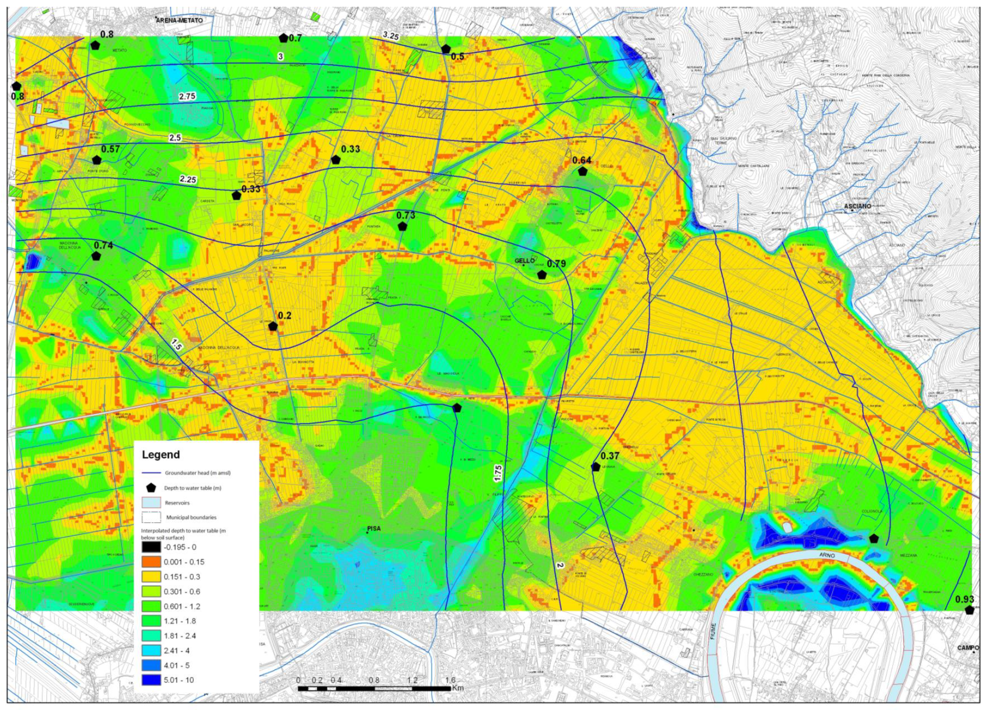
28], generally constituted by fine alluvial sediments (sand passing to silt and clay), brought by the Serchio and Arno rivers. These aquifers show a shallow water-table (up to 4 m depth;
Figure 3). Because of this, a large part of the area is mechanically drained to prevent waterlogging. The groundwater hosted in these aquifers, although not used for drinking purposes, is often used for irrigation and domestic purposes [
29].
We reasonably assumed homogeneity of the climatic characteristics (as regards to the distribution and intensity of rain events) and of the agronomic practices (doses and distribution methods) in the investigated domain.
2.3. Application of the VI Method
In the investigated area, pesticide use showed a large variability in space and time, being driven by crop rotation on farmland, by the type of weed (or other target organism) community (composition and numerosity), and by practical considerations (costs, market availability, farm stocks, etc.). Therefore, we should have prepared 33 different maps, one for each AI detected within the case-study area. Rather than this, we used an approach based on grouping the active ingredients into classes, in agreement with Schlosser et al. (2002) [
22]. This way, we simplified the data processing to achieve an overall analysis of the specific vulnerability of the shallow aquifer to pesticides. These classes were defined based on the leaching ratio (LR) of each active ingredient. The LR, embedded in the VI model, expresses the potential leaching for each compound throughout the soil and is based on transport properties of an active principle (such as biochemical degradation and sorption). The LR is defined as:
Therefore, the leaching ratio constitutes an estimate of the susceptibility of each AI to be biodegraded and to be sorbed to the soil organic matter. The longer the half-life, the less degradation the compound will undergo moving through the soil, and a larger mass of active principle will therefore be expected in groundwater. Pesticides with a high t1/2 will result in a higher LR and will determine a greater vulnerability for the area where they are used. On the other hand, compounds with a high KOC will exhibit a larger tendency to sorption. Therefore, they will require more time to reach the water table, consequently allowing longer times for degradation and, finally, a lower expected mass in groundwater.
The 33 AIs presented in the previous section, were divided into three leachability classes (respectively low, medium, and high) based on the LR ratio (
Table 5 and
Table 6). Following [
22], AIs with a ratio lower than 0.01 were assigned to the "low" class, with a ratio between 0.01 and 0.1 to the "middle" class, and those with a ratio greater than 0.1 to the “high” leachability class. For each of these three classes, a specific vulnerability map to pesticides was then produced.
The analysis carried out was performed within the municipal boundaries only for the domain where piezometric data were available.
2.4. Model Parameterisation
We describe here the parameters used for applying the model to the case study. Unfortunately, the availability of the parameters needed for the application of the VI index method (Equation (1)) was limited to the main soil typology identified within the case-study area (in the number of few units). Therefore, it was necessary to apply the same value of the parameters K and θFC to each polygon belonging to a specific type of soil. For the parameters Z, ρb, and %OM a single value was assigned to all the investigated domain. Afterwards, we transformed the vector data files in raster data in order to process these parameters with those available in raster format, and then we calculated the VI index by performing raster analysis calculations in the GIS environment for each class of pesticides.
2.4.1. K, Soil Saturated Hydraulic Conductivity
The parameter K, hydraulic conductivity, is used in the model as a surrogate for the soil-water velocity assuming a unit hydraulic gradient (gravity-dominated flow) for near-saturated conditions as during irrigation [
22]. K data were assigned to each class of soil and were derived from [
26].
2.4.2. θFC, Water Content at Field Capacity
For the purposes of this analysis, one θ
FC data was assigned at each type of soil in the study domain and the data was derived from [
26].
2.4.3. Z, Thickness of the Soil Layer
This parameter corresponds to the thickness of the soil layer, where most of the sorption and biodegradation processes occur (hence, it is not the thickness of the unsaturated area). It is well known that most of the organic matter and biological processes usually occur in the shallowest layers of the soil. In this case, since spatial-distributed data of this parameter were not available, we choose to assign a single value, equal to 1 m, to the entire study domain on the basis of the soil nature and the usual soil tillage depths. As such this parameter did not impact the calculation of the VI in different areas of the investigated domain.
2.4.4. ρb, Soil Bulk Density
Only two tests were carried out for the soil bulk density during the soil map survey [
26]:
- —
one on the STF1 soil, with an average value ρb = 1.53 g/cm3.
- —
one on the GRE1_STG1 soil, with an average value of ρb = 1.49 g/cm3.
As no further data were available to characterize the other soil types, a single value equal to ρb = 1.5 g/cm3 was assumed and assigned to the study domain. Also, in this case, this parameter did not impact the calculation of the VI in different areas of the domain investigated.
2.4.5. %OM, Percent Organic Matter
Regarding the organic matter content, results from two samples were available. They showed an average organic matter content of 3.24% and 5.6% respectively. Since only two data points were available, and rarely organic-rich soils are found in the study domain, a single value of 3% organic matter content was assigned to the whole domain. In this case, this parameter did not impact the calculation of the VI in different areas of the investigated domain.
2.4.6. Leachability Ratio
We associated to each group of pesticide the median value of the leachability ratio for each of the classes as defined in
Table 5.
2.4.7. The FDGW Parameter
This dimensionless factor accounts to the depth to groundwater, as this distance may influence the amount of pesticide that reaches the water table. Larger values of the parameter were assigned to areas where the unsaturated zone had a small thickness, while smaller values were assigned where the thickness was large, by using a non-linear relationship.
Using the piezometric survey data (from [
30]), we prepared a depth to water table map by subtracting the values of the groundwater head to those of the surface elevation derived from the Tuscany Region digital terrain model (10 m cell). Results were processed using a Kriging interpolator. In some areas, a negative depth to water table value was obtained as a result of the interpolation process. As it was not possible to validate these data with extensive experimental campaigns, we assumed a precautionary depth to water table of 0.15 m for all the areas where the interpolated value was lower than 0.15 m. The final depth to water table map is presented in
Figure 3. As already mentioned, the analysis carried out was only performed for the domain where piezometric data were available. In [
22] the F
DGW parameter was assigned according to the scale presented in
Table 7. In order to assign a higher score to depth to water table values less than 2 m from the soil surface and often close to zero (a frequent situation in our case study), we built a non-linear relationship according to which as the unsaturated thickness decreases, the value of the F
DGW parameter increases following an exponential function. This relationship allowed us to assign a greater F
DGW value to the areas with very small depth to water table. The curve derived is shown in
Figure 4. The parameter values then assigned for the different areas are reported in
Table 8, while in
Figure 5 the map with the spatial distribution of the F
DGW parameter is presented.
3. Results and Discussion
We applied the VI model to the three leachability classes of pesticides in the investigated area. Although the original method identified three vulnerability classes (
Table 1), we added a fourth class of vulnerability to highlight areas with a value of VI greater than 1000. This new class included all areas characterized by a very high level of aquifer vulnerability.
The results are presented in the form of specific vulnerability maps for the three leachability classes of pesticides previously defined and discussed below in
Figure 6 and
Figure 7, except for the class of pesticides with a low leaching ratio. In the latter case, the vulnerability index calculated for the entire investigated area was low. This low vulnerability class was maintained in all areas, even performing calculations with a lower organic matter content, 2% instead of 3%.
Regarding the medium leaching ratio pesticide class (
Figure 6), the interaction between the nature of the AIs and the physical-chemical characteristics of the soil led from medium to high areal distribution of vulnerability, whereas the zones with low vulnerability resulted in very small areas. Comparing this map with the soil distribution map (
Figure 2), the influence on the result of the parameters assigned specifically to each type of soil, and particularly of the
K parameter, can be seen.
Finally, the vulnerability to the class of pesticides with a high leaching ratio (
Figure 7) varies from medium to very high, demonstrating the need for careful use of these kind of agrochemicals by the farmers. The consistency of our estimates was strictly dependent on the density and spatial distribution of the data used. In fact, we derived several of the input data from soil maps with little experimental information collected in the investigated area. The scarcity of experimentally gathered data mainly limited the predictive value of the vulnerability classification of the study area. In fact, our results may be considered an initial screening that might be used to provide general advice on pesticide use, especially under high or very high vulnerability index conditions. We also suggest that in such areas experimental activities are run to monitor the use of pesticide on farming practices and their potential leaching following distribution. In terms of uncertainties in the parameters, while Z, ρ
b and %OM may not show a large variability range in the investigated area, this is not the case for
K. This parameter may vary up to an order of magnitude, impacting the definition of the vulnerability classes. Anyway, further data on the characteristics of the soils (primarily the organic carbon content) would allow us to, for example, better rate the vulnerability score in areas with high organic matter.
Concern is also expressed in relation to the fact that in the investigated area the water table is very shallow, and consequently the barrier effect and the attenuation provided by the soil and the unsaturated zone bio-geochemical processes might be ineffective. It must be mentioned that as the area is mechanically drained, the worst-case scenario would be depth to the water table equal to zero (waterlogging). This could happen during very wet seasons. In that case, all the areas would be rated from high to very high vulnerability, notwithstanding the class a pesticide is attributed to.
Furthermore, performing groundwater monitoring and sampling to detect the presence of active ingredients, besides shedding a light on the real groundwater chemical status respect to pesticide presence, is a necessary step to validate the maps produced.
Although the proposed method is based on a small number of parameters compared to other methods, the required parameters are time-consuming and expensive to obtain. This means that to produce a sound, but static, vulnerability assessment, the cost in data gathering may be high. We then suggest that index-overlay methods for vulnerability mapping are combined with process-based methods such those offered by numerical modelling. Freely available and open source software tools (such as Hydrus 1-D [
33]; the SID&GRID [
34] or FREEWAT suite [
35,
36,
37]; VLEACH [
38], etc.) are widespread and allow implementation of dynamically improving models which may be able to not only validate the maps produced, but also to help in redefining areas at different vulnerabilities based on simulated processes and associated uncertainties. Thus also increasing the data value and better justifying the cost for large dataset acquisition [
39].
4. Conclusions
Evaluating the risk of pesticide leaching into groundwater is a necessary step to suggest robust advices on the usage of such compounds in agricultural practices, hence reducing groundwater contamination risks and supporting cropping system sustainability. However, choosing a proper method for the assessment of such risks is not straightforward. In this study, we applied the vulnerability index method [
22] as an example of an index-overlay method. This method needs a relatively small number of parameters compared to other more complex ones. Yet, even such a small number of parameters was not easily available in our case study. Several data had to be derived from soil maps and then averaged over large areas. This lead to vulnerability maps with reduced reliability, no validation with groundwater samples for the presence of active ingredients, and little practical use. We then suggest that maps produced in such way may provide information on specific vulnerability in areas identified as at high risk of leaching. In such areas, a specific focus should be on delivering advices to farmers on the use of pesticides, and at the same time monitoring the impact of such use. Here, we want to reiterate how extension services for farmers and owners of plant nurseries and greenhouses in the correct use of agrochemicals is, however, the first and most important action for the protection of water resources.
Finally, the cost for producing reliable static vulnerability maps based on index-overlay methods can be high, because of the several data that need to be gathered. The value of these data may, however, be increased, and the cost better justified, if the analyses are carried out by using process-based or advanced statistical methods. While the future for vulnerability assessment methods is in process based/advanced statistical methods, index-overlay methods, as a preliminary step for process-based simulation analysis, may still provide initial and quick insights into potential leaching of pesticides to shallow aquifers.


