1. Introduction
Irrigated valleys represent only 20% of the world’s cropland, but on the other hand, they produce 40% of the global crop harvest. In intensively cultivated areas where the soil is dry, irrigation improves economic returns and can boost food production by up to 400%. Efficient irrigation systems and water management practices show an alternative to deal with soil conditions in arid and semi-arid cropland surfaces [
1]. Good agronomic practices are also needed to manage the natural resources around the world. The amount of water for irrigation purposes as well as for the crops yield and the size of the cultivated areas must be determined in order to estimate the available food for all humankind [
2].
The Bonaerense Valley of Colorado River (BVCR) is an irrigated cultivated area located in the south of Buenos Aires Province, Argentina. Among different crops present in the area, onion and sunflower have a high regional economy impact with thousands of cultivated hectares. Due to this economic significance and also the objective of maximizing the efficiency of agriculture activities using good agronomic practices, it is crucial to know—as precisely as possible—the cultivated area size and the spatial distribution in order to manage the natural resources properly. Thus, in the context of SDG 2030 (Sustainable Development Goals), reliable procedures to estimate the land use expanse at local and regional scales are necessary for a sustainable management of onion and sunflower crops [
3].
The BVCR is the main onion crop production area in the country (65% of the planted hectares in the country) with a large participation in the regional economy, supplying not only the Argentinian domestic market, but also meeting the international demand. Due to the international market regulations, the BVCR’s onion crop complies with high quality standards. According to the sowing estimations, between 8000 to 9000 hectares are sown every year in the region. The sunflower crop has great yield levels in the Colorado River valley intensively cultivated area. The sunflower hybrid seeds have high fat matter content very suitable for high quality oil production. This crop characteristic is very attractive for the national and international seed companies [
4].
Crop yield in the BVCR is extremely related to soil moisture and nutrients. Water availability and suitable soil conditions are crucial factors in plant growth, which enable a high-quality product [
5]; the possibility of implementing technologies that improve productivity drives the achievement of a substantially lower cost per kilogram than other areas in Argentina. Given this panorama, it is important to carefully manage the natural resources, soil and water, but also to optimize the producers’ economic resources.
Determining the location of crops and their spatial coverage dynamics, as well as estimating their area before harvest, has a strategic value for the commercialization of BVCR products in the domestic market and in MERCOSUR [
6].
Earth Observation Systems (EOS) provide unprecedented opportunities for a reliable monitoring of cropland activities, especially in inaccessible areas and intensively cultivated agricultural fields. In recent years, the possibility to access multiple classification algorithms and sensor images with a higher spatial (SPOT) and spectral (Sentinel-2, S2) resolution have encouraged the increase of new lines of research.
Land cover maps derived from optical images in an irrigated valley have been assessed employing S2A images [
7]. To select the optimum vegetation index (VI) in order to build crop masks, field radiometry and SPOT 6 and 7 high spatial resolution images were employed to quantify the onion crop surface in an intensively cultivated area [
8]. The classification statistical results, overall accuracy (OA) and Kappa index (Kp) are strongly related to the optical satellite image date. To mitigate this optical satellite image date dependency, temporal series have been used to classify different crops [
9]. A plant’s phenological state depends on the crop environment and season date [
10]. The use of optical satellite imagery is limited by the availability of cloud-free images. When the wet season takes place during a warm season, or summer, rain falls mainly during the late afternoon and early evening, affecting mostly the optical sensors on board remote sensing satellites. Thus, the optical time series imagery is limited by the crop dry season and the classification methods must deal with short image datasets and uncompleted crop phenological cycles, making it difficult to train the supervised algorithms efficiently.
Sentinel-1 (S1), as the first satellite constellation of the European Space Agency’s (ESA) Copernicus programme, provides cloud and season independent data about land surface features. S1 is a C-band Synthetic Aperture Radar on board the satellites S1A and S1B, offering 6 to 12-day revisit-time images. The ESA S1 observation strategy defines the Interferometric Wide swath (IW) mode as the pre-defined mode over land. This mode provides dual-polarization (VV and VH) imagery, at a resolution of 10 m, with a swath of 250 km [
11]. Copernicus offers free access products and a fast delivery system.
Synthetic Aperture Radar (SAR) time series imagery enhances day and night crop development stage monitoring, even in rain or dust weather conditions, for all seasons of the year. This condition makes S1 SAR data suitable for vegetation biophysical parameters retrieval. Land cover maps can be derived also from SAR imagery, favoring the benefits of the machine learning algorithms during the training stage.
SAR data have been widely used for different applications, from mapping cropland cover to retrieval of vegetation parameters such as height and biomass [
12]. The C-band SAR VV polarization signal is often dependent on soil moisture, which is related to its dielectric constant and surface roughness. The SAR VH polarization signal interacts primarily with the vegetation structure and canopy layer only to a limited extent. S1 SAR time series have been used for monitoring the complete summer (maize, soybean and sunflower) and winter (rapeseed, wheat and barley) crop phenological cycles. The correlation between the NDVI derived from S2 optical imagery and the ratio VH/VV obtained from S1 was shown by Veloso et al. [
13]. S1 and S2 temporal series synergy presents a strategy to reconstruct wheat and tomato Leaf Area Index (LAI) values over the agricultural fields region of Foggia, Italy, where optical S2 cloud-free image availability is constrained by weather conditions [
14]. For land cover classification purposes, texture measures from a Grey Level Co-occurrence Matrix (GLCM) provide reliable information on the spatial relationship of the image pixels feature and their spatial and structural distribution in the landscape [
15]. The specular pattern and texture information extraction from SAR images are essential metrics for cropland cover classification tasks, having a direct influence on the reliability of the statistical results of SAR image classification.
S1 imagery for classification purposes has been applied in different places in the world such as India, Africa, France and Spain [
16]. These investigations have shown that crop growth can be monitored, with improved results from radar backscatter, in different environmental conditions [
17], especially with cloud cover [
18], obtaining good results using a Support Vector Machine (SVM) and Random Forest (RF). S1 SAR data has been also assessed in winter crop classification [
19], in horticulture [
20] and in water and soil management [
21].
The capacity of high resolution C-band S1 SAR (VH+VV polarizations) time series data for land cover classification in the BVCR’s crop campaign was assessed considering different crops present in the study area, and onion and sunflower showed a high reliable discrimination performance based on classification statistical results for OA and Kp [
22]. For image classification objectives, GLCM texture features derived from SAR time series imagery provide reliable information regarding the cropland structure in the landscape [
15].
This research aimed at assessing the potentiality of C-band high resolution SAR data, polarization and GLCM texture features from multi-date S1 images, to differentiate onion from sunflower crops, among others, in the BVCR valley. Based on GLCM, we used four texture measures, contrast, correlation, entropy and variance, to capture the pixel spatial relationships in a SAR image. The speckle inherent effect was eliminated by calculating the median value at the crop lot level. We evaluated two machine learning algorithms, RF and SVM, for discriminating land cover types. As a complement, the results obtained from the combination between SVM and RF, using the logic of the maximum vote and the contribution of the principal component analysis (PCA) in reducing the S1 SAR features database dimension, were analyzed.
The proposed classification method presents an alternative to pixel-based approaches, improving the crop class integrity at lot level and reducing the SAR speckle noise over the whole mapped area.
2. Materials and Methods
2.1. Theoretical Background
2.1.1. SAR C-Band for Crop Monitoring
Synthetic aperture radar has great potential for monitoring vegetation biophysics parameters [
23,
24,
25]. It allows day and night image acquisition of all-weather conditions. Yet, in tropical and similar rainforest regions elsewhere, the use of optical satellite imagery is often limited to cloud-free images collected in a dry season.
The C-band SAR penetrates the vegetation canopy only to a limited extent and interacts also with the soil [
26]. The radar backscatter signal is affected by factors related to crop biomass and the three-dimensional vegetation structure [
27] as well as by the ground conditions and the radar configurations used for the observations [
28]. Previous studies [
29,
30,
31] have shown that the backscatter’s coefficient value in C-band is a combination of the soil backscatter attenuated by the canopy layer and the backscatter from canopy, which includes simple and multiple scattering, and finally the vegetation-soil interaction [
32]. Other factors that contribute to the soil backscatter value are soil moisture, the surface roughness and terrain topography [
7], which is the reason why SAR data sensitivity to soil moisture could be useful to detect irrigated crops.
In terms of incidence angle, those between 35° and 40° increase the path length of the radar signal through the vegetation and maximize the scattering contribution produced by the vegetation structure [
33], while incidence angles lower than 30° increase the ground scattering distribution, which contributes to assessing the soil moisture [
34].
At the beginning of the crop season, the radar signal interacts only with bare soil surfaces, and the radar backscatter is affected mainly by the moisture and roughness of the soil. The VV polarization, more sensitive to superficial scattering, is appropriate to determine the bare soil properties in this crop phenological cycle stage [
35]. When the vegetation starts growing, the radar signal interacts with the emergent plants, which produces a backscatter increase. In the crop growing stage the VH polarization, more sensitive to volumetric scattering, is optimum to follow the vegetation phenological cycle. When the harvest takes place, the VH signal remarkably decreases due to the bare soil condition. In this stage, the backscattered superficial energy increases, which can be detected by the VH polarization [
36]. So far, few studies have used dense time series SAR data for crop monitoring. Only recently, S1 data have been used [
37,
38].
The performance of a supervised crop classification approach based on crop temporal signatures obtained from Sentinel-1 time series imagery in the Spanish province of Navarre was studied by Arias et al. [
39]. They considered 14 crop classes including winter and summer crops. In those cases where the three S1 SAR features (VH, VV and the ratio VH/VV) were used, the OA values obtained were higher than 70%. In-season soybean crop mapping over Ujjain district, Madhya Pradesh, was addressed by Kumari et al. [
40]. They found a correlation between the temporal characteristics of soybean crop and the smooth VH backscatter profiles. The SVM algorithm was used to classify the S1 data into soybean and other crops, reaching OA values of more than 80%.
In the Hebei Province of China, corn crop was mapped using multitemporal S1 SAR data and S2 optical images in the Google Earth Engine (GEE) cloud platform. A total of 1712 scenes of S2 data and 206 scenes of S1 data were processed to composite image metrics as input to a RF classifier. To avoid speckle noise in the classification results, the pixel-based classification result was integrated with the object segmentation boundary to generate an object-based corn map according to crop intensity [
41].
2.1.2. Grey Level Co-Occurrence Matrix
SAR texture information features can be extremely useful for image classification. Considering the spatial information present in the SAR image, new texture images can be reconstructed. Texture shows the intensity variations in an image and can contribute to improved land cover classification accuracy. Texture features involve information from neighboring pixels, which is important to characterize the identified different crop types in agricultural fields.
The Gray Level Co-occurrence Matrix (GLCM) proposed by [
42] is one of the most widely used methods to compute second order texture measures. Several texture features can be computed from the GLCM matrix. Each feature model produces different properties of the statistical relation of the co-occurrence of pixels estimated within a given moving window and along predefined directions and inter-pixel distances. The GLCM is a measure of the probability of occurrence of two grey levels separated by a given distance in a given direction,
θ. Each element value of the GLCM is calculated as follows:
where
P (
i,
j,
d,
θ) is the frequency of the double element point, one of which is the pixel grayscale value
i, another pixel grayscale value of
j, and the adjacent distance to
d in
θ direction.
For SAR image classification, the following four parameters are taken for quantitative description of the image texture condition based on the GLCM [
43,
44,
45].
Variance
The variance texture parameter is focused on the partial characteristics of the SAR image.
where
p(
i,
j) is the (
i,
j)th entry in a normalized gray-tone spatial dependency matrix
p(
i,
j) =
P(
i,
j)/R and R is a normalizing constant; µ is the mean value of the p matrix. Ng is the number of the distinct grey levels in the quantized image.
Contrast
The contrast feature is a difference moment of the P matrix and is a measure of the number of local variations present in an image [
42]. Contrast shows the change total quantity of partial gray graduation in the image. For instance, the contrast feature for a grassland image has consistently higher values compared to a water body image.
Correlation
The correlation feature is a measure of gray-tone linear dependencies in the image and it describes the similarity among the elements of columns or rows in the GLCM. The p
x(i) and p
y(i) are the (i)th and the (j)th entries in the marginal-probability matrix and can be obtained by summing the rows or columns of p(i, j) respectively.
The expression of the GLCM correlation feauture can be shown as follows:
where
µx,
µy,
σx and
σy are the means and standard deviations of
px and
py given by Equations (4) and (5)
. Entropy
The entropy feature determines the abundancy degree of image information. The size of the entropy represents the average image information.
2.2. Study Site
At the coastal land of the Colorado River in Buenos Aires Province, Argentina, in the sixties, significant transformations began in the natural landscape. The BVCR is located between the 39° and 40° south latitude parallels and the 62° and 63° west longitude meridians. The area has a surface of 500,000 ha, of which 140,000 ha are irrigated by an extensive irrigation network and an uncoated drainage channel [
34]. The studied area corresponds to a 50,000 ha area located in BVCR in the Villarino district in the south of Buenos Aires Province (see
Figure 1).
Gravity irrigation has made most of the agricultural activities in the area possible. The horticulture specialized in onion (Allium cepa), squash (Cucurbita pepo) and potato (Solanum tuberosum) stands out. Other crop types present in the BVCR are alfalfa for seed and haymaking, maize (Zea mays) for seed and silage, sunflower (Helianthus annuus) for seed [
46], winter cereals such as oats (Avena sativa) and wheat (Triticum durum), as well as forage pastures. The implanted crops under irrigation condition occupy 91,163 hectares in the BVCR, including horticulture, pastures and cereals. Among other vegetables that can be found in the BVCR, onion is the main crop with an average cultivated area from 10,000 to 13,000 hectares per year [
3], with an average yield from 40 to 50 tons [
47]. Currently, this microregion is the main hybrid sunflower seed producing area in the country, with a sown surface size ranging from 8000 to 10,000 hectares per year, approximately 90% of national production.
2.3. Characteristics and Environment of Onion and Sunflower Crops in the BVCR
In the BVCR, onion crop represents 58% of the regional agricultural gross product, between 32% and 48% is exported, and the remainder is delivered to the internal market [
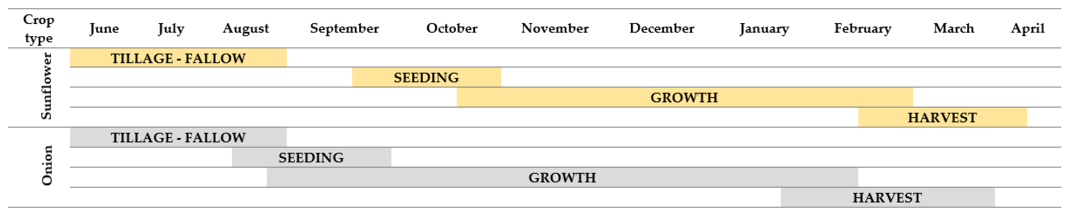
48]. The Valenciana variety has a long phenological cycle, it is sown from July to August and the harvest takes place in February [
49,
50]. Between November, December and January, a higher irrigation frequency is required by the different crops present in the valley, mainly by the onion crop, with an average of 19 to 22 irrigations reaching 100 mm/ha of irrigation water in all the vegetative cycle [
51]. Traditionally, irrigation through a pumping canal system has been used in the region. In recent years, different methods like sown flat area and irrigation terraces have considerably increased [
8]. Due to the superficiality of the root system, the onion roots do not explore the soil profile beyond a depth of 30–60 cm, and it is necessary to increase the irrigation frequency [
52,
53]. Furthermore, there are other crops under irrigation such as alfalfa, sunflower, maize and winter cereals with a lower irrigation request, between 3 and 5 irrigations per cycle. From August, the long day onion sowing begins. In mid-October or during the first days of November, it is possible to find emerging seedlings. The harvest is made from the end of January until the end of March. The highest vigor of the vegetation is produced at the end of December, and later, the senescence and maturity begin. In March, the great onion percentage is harvested.
Sunflower cultivation was introduced in 1995 as an industrial crop and nowadays production has been almost completely converted to hybrid seed production. The BVCR environment is very suitable for sunflower production. It is a semi-arid climate, with long days in summer and high sun radiation. Soils are deep, irrigated and poor in fertility. These conditions allow an optimal sanitary sunflower condition. The sunflower’s photosynthetically active leaf area is exposed to sun radiation for long periods of time, encouraging grain yields greater than 5 t/ha and high seed fat matter content (about 59%) [
54]. The production modality is made through contracts between the seed companies and the farmers of the valley [
55]. High quality seed production stands out for yields that vary between 1200 kg/ha and 2400 kg/ha. Regarding crop profitability, normally the seed value is 4 to 5 times greater than the common price [
56]. The hybrid sunflower seed is produced from male lines (pollen producers) and female lines (male sterile), and fertilization necessarily requires bee pollination services, which are present in the area, adding one more activity to the local economy (see
Figure 2). From the use of water and nitrogen resources point of view, it is important to highlight the sunflower crop as an excellent successor to the onion crop. Onion crop has shallow roots and requires a lot of nitrogen and water, approximately 20 gravitational irrigations, and water and nitrogen surplus percolates to the deepest profiles of the soil where the sunflower crop can take advantage of it.
For sunflower cultivation success, the pre-sowing and irrigation in the V12 (12 green leaves per plant) vegetative state are considered essential. Then, depending on the depth of the water table and the amount of precipitation during the growing stage of the sunflower buds, it may require 1 or 2 additional irrigations, at the beginning of the first phase of seed fill. In the valley region, the rotation sequence, pasture-onion-sunflower-wheat-pasture, is considered sustainable in the context of good management of agronomic practices.
For sunflower, the tilling labours begin in July. The optimum sunflower sowing date in the BVCR is in October, considering its expected yield performances [
56]. While seeding may occur in the third week of September, it is not advisable, not only because of the eventual freeze the crops might suffer but also because a significant delay in the seeding itself is registered (by three weeks), which exposes it to a higher grade of damage produced by pigeons and insects and because of competition with weeds. From the middle of October to the end of February, the sunflower growing is ongoing, and plants reach a height of 2 m in the study area. From the middle of February to the middle of April, the sunflower harvest is done in the BVCR (see
Figure 3).
2.4. Irrigated Valley of Colorado River Soil Taxonomy Classification
In the BVCR area where the irrigation is gravitational, the soil experiences two issues that are directly related to the crop productivity. The first is soil salinity, which is associated with poor irrigation water drainage. The second is soil cutting, which originates from beheading the first centimeters of the soil (performing the labour of matching the surface to obtain an optimal drainage) where the most favourable nutrients for the crops are present.
According to soil taxonomy classification [
57], the soil groups present in the study area are the following: Typic Haplustolls, Entic Haplustolls, Molic Flucolic, Aquic Hapludolls, Cumulic Hapludolls, Mollic Ustifluvents, Haplargids and Natrargids. These are generally coarse soils, mostly sand to sandy loam, with low organic matter content (around 1%), medium to high phosphorus supply (between 10 and 30 ppm) and high potassium content (between 200 and 1000 ppm).
The soils in the BVCR are also very susceptible to wind erosion [
58,
59,
60]. The soils of the irrigated area have been modified by the practice of gravity irrigation. Below the first loose layers are horizons with fine deposited material such as silt and clay, sometimes overlapping. The presence of consolidated calcium carbonate does not generate a problem for the roots. There are mainly three representative soil series in the study region (see
Table 1 and
Figure 4).
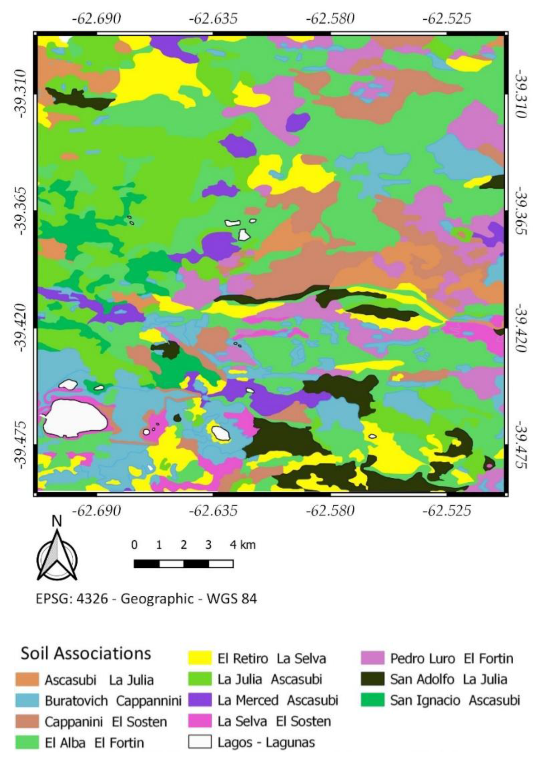
The soil series involve the most common soil component having a unique combination of properties that distinguish it from neighboring series. It is the lowest categorical level of soil taxonomy. Secondary soil series derived from the three main soil series present in the area can be found in the irrigated valley of the Colorado River study site. The secondary series are the following: Ascasubi, Buratovich, Cappanini, El Alba, La Julia, La Merced, La Selva, Pedro Luro, San Alfonso, San Ignacio and El Retiro. In the study site, 11 soil associations can be distinguished. Soil association is a map unit consisting of two or more dissimilar soil major components occurring in a regular and repeating pattern on the landscape [
57]. In the BVCR the soil associations are composed mainly of two secondary soil series. The soil associations composition is shown in
Table 2.
The soil map of the study site thus consists of soil associations map units meeting the criteria for the taxonomic class (see
Figure 4).
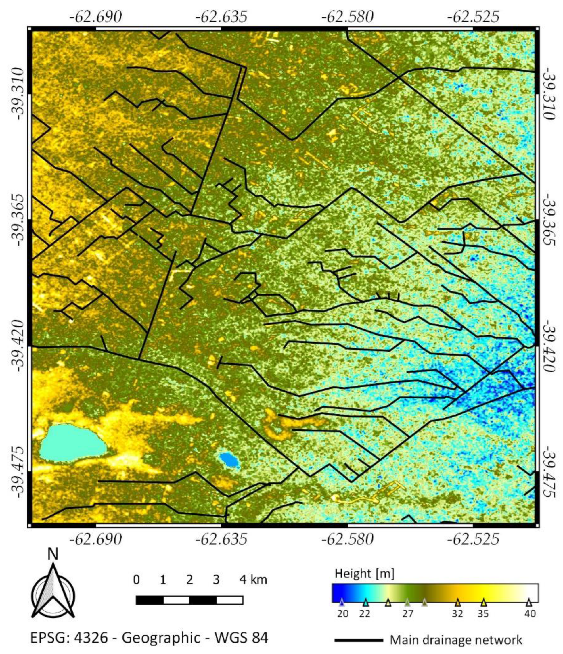
Slopes in the region range from 0 to 1%. The slope in this region descends from the west towards the east. The maximum ground height difference (above sea level) is roughly 20 m in eighty kilometers (see
Figure 5). The extremely soft slopes in the irrigated area produce low surface runoff capacity in the drainage channels. The depth level of the water table is about 1.2–1.4 m in the irrigated cropland and relatively deeper in the dry area, which degrades the soil through salinization processes.
2.5. Field Data for Training and Validation
During the 2017–2018 crop campaign, expert professionals and technicians of INTA (Agricultural Technology National Institute), Argentina, performed a ground field measurement campaign to register the different land cover types in the irrigated valley of the Colorado River intensively cultivated area. Four field observation transects were scheduled between August and November 2017. The GT (Ground Truth) database has 1634 registers, each one corresponding to a measurement point. Two different methods were used in collecting data. Firstly, direct observation of land coverage and, secondly, optical analysis based on satellite image texture and historical databases. A total of 916 ground truth direct observations were taken in the study zone, the land cover types were registered in a database, as well as other parameters related to the 2017-2018 crop campaign. The GT points positions were determined with GPS equipment. Photographs were taken, and the most relevant crop aspects were registered on a database. The optical analysis was done on a set of SPOT 5, 6 and 7 images provided by the CoNAE (National Committee of Spatial Activities) using different products: panchromatic band, RGB composition and a fusion (pan sharpening) of both. A high spatial resolution of 1.5 m was used to distinguish the different land cover types. Based on a high resolution SPOT 5 image from October 2016, the parceling of lots, the irrigation-drainage infrastructure and the communication channels in the prioritized area of 50,000 ha were digitized. Thirteen thousand polygons were added to a vector type layer. It was possible to discriminate a new 620 land cover points by using a set of SPOT 6 and 7 images. Once the onion crop cycle is finished, it is gathered manually or mechanically, and it differs from the rest of the crops because of its texture and shape. These aspects can be clearly visualized in the optical images of SPOT 6 and 7 (see
Figure 6). Furthermore, there is a historical database with land cover not suffering modification such as the hills, resting and neutralized fields that are added to comments from the owners of different lots of the BVCR that provided information. Thus, 98 additional points of land coverage were obtained [
61,
62].
2.6. Sentinel-1 C-Band High Resolution SAR Data
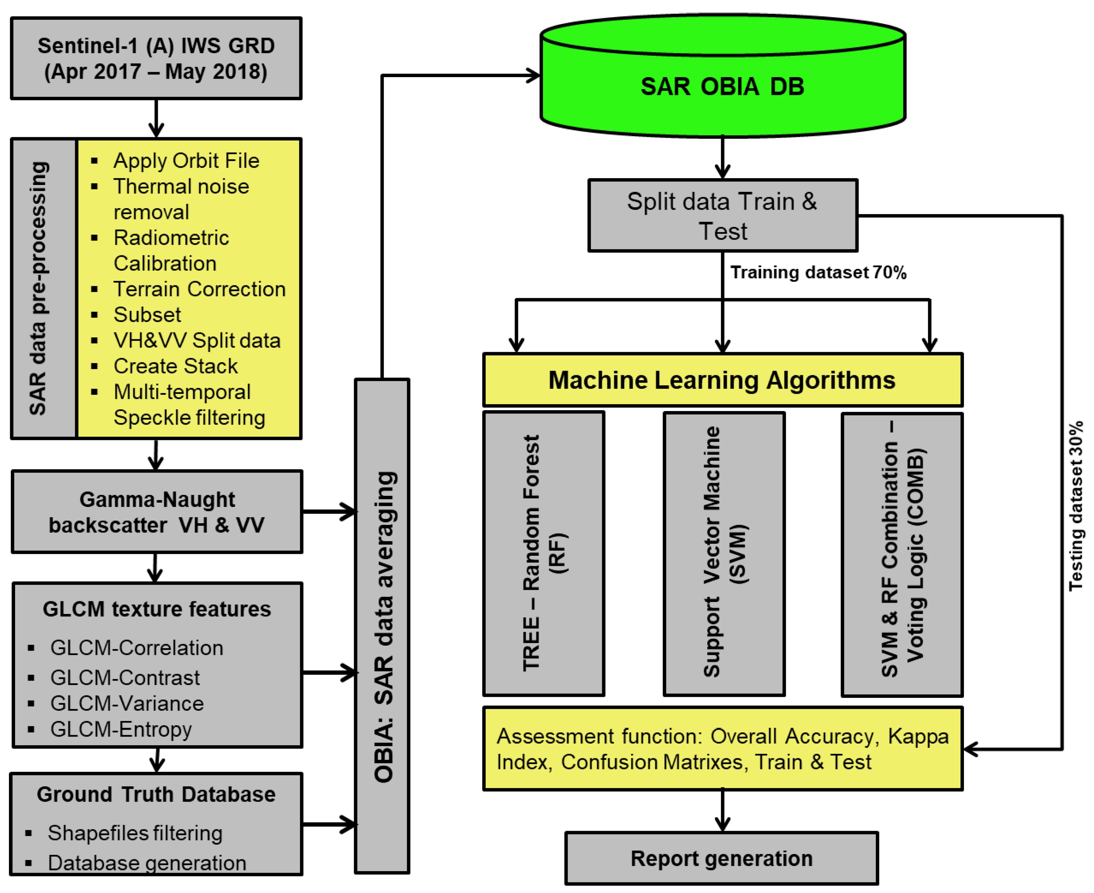
A S1 image automatic-processing chain was implemented in SNAP (Sentinel Application Platform) version 7.0, using the Sentinel-1 Toolbox and the GPT module (Graph Processing Tool). A processing script in Bash (Bourne-again shell) language was developed in a Linux environment. Sentinel-1A GRD (Ground Range Detected) products in IWS (Interferometric Wide Swath) mode, available in dual polarization VV+VH, were selected for the analysis providing a 12-day revisit time over the study site. A total of 30 S1A images between April 14, 2017, and May 15, 2018, were downloaded from the Copernicus Open Access Hub web site (
https://scihub.copernicus.eu/). The selected relative descending orbit number is 141. The acquisition time of S1 over the study area is around 9:20 h local time. The incidence angle over the monitored cropland region varies from approximately 38° to 41°. The GRD Level-1 products consist of focused SAR images averaged by multi-looked methods and ground projected using the WGS84 reference system. First, the data were calibrated to obtain the normalized backscatter coefficient γ
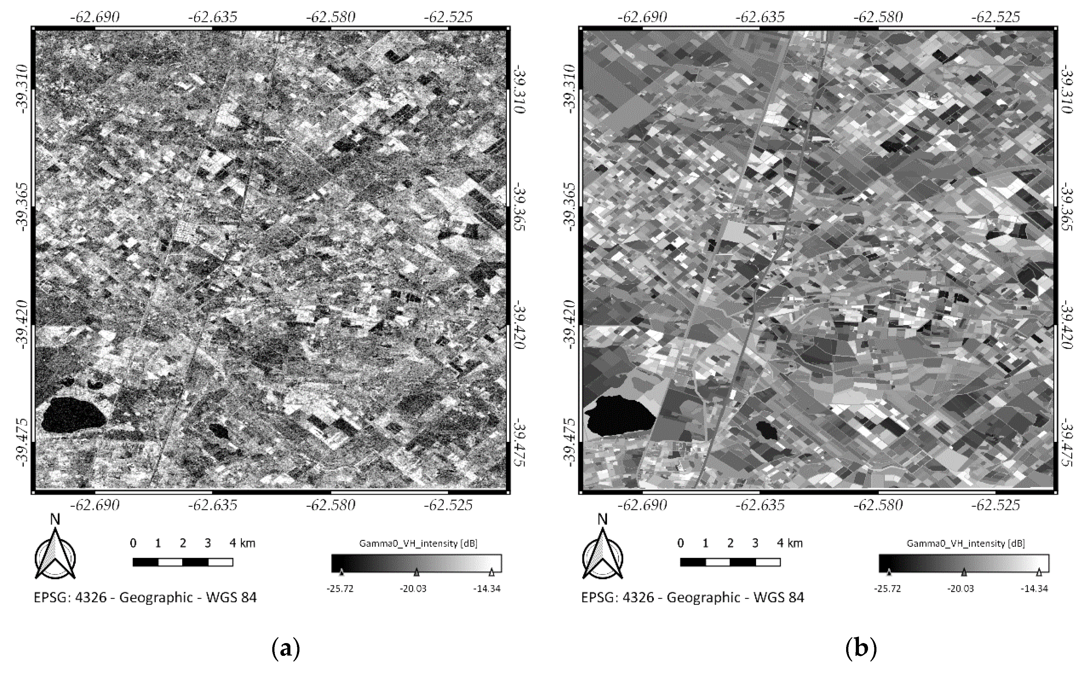
0 (Gamma Naught). No additional multi-looked processes were performed, whereby the spatial resolution for the S1 IWS-GRD product is 10 m. Therefore, the range doppler terrain correction was applied to geocode the images precisely using the SRTM (Shuttle Radar Topography Mission) digital elevation model. Finally, the images were overlapped without an additional co-registering process in order to create a time series stack. A multi-temporal speckle filtering process was applied to the VH+VV polarizations stacks. An IDAN filter (Intensity-Driven-Adaptive-Neighborhood) was used [
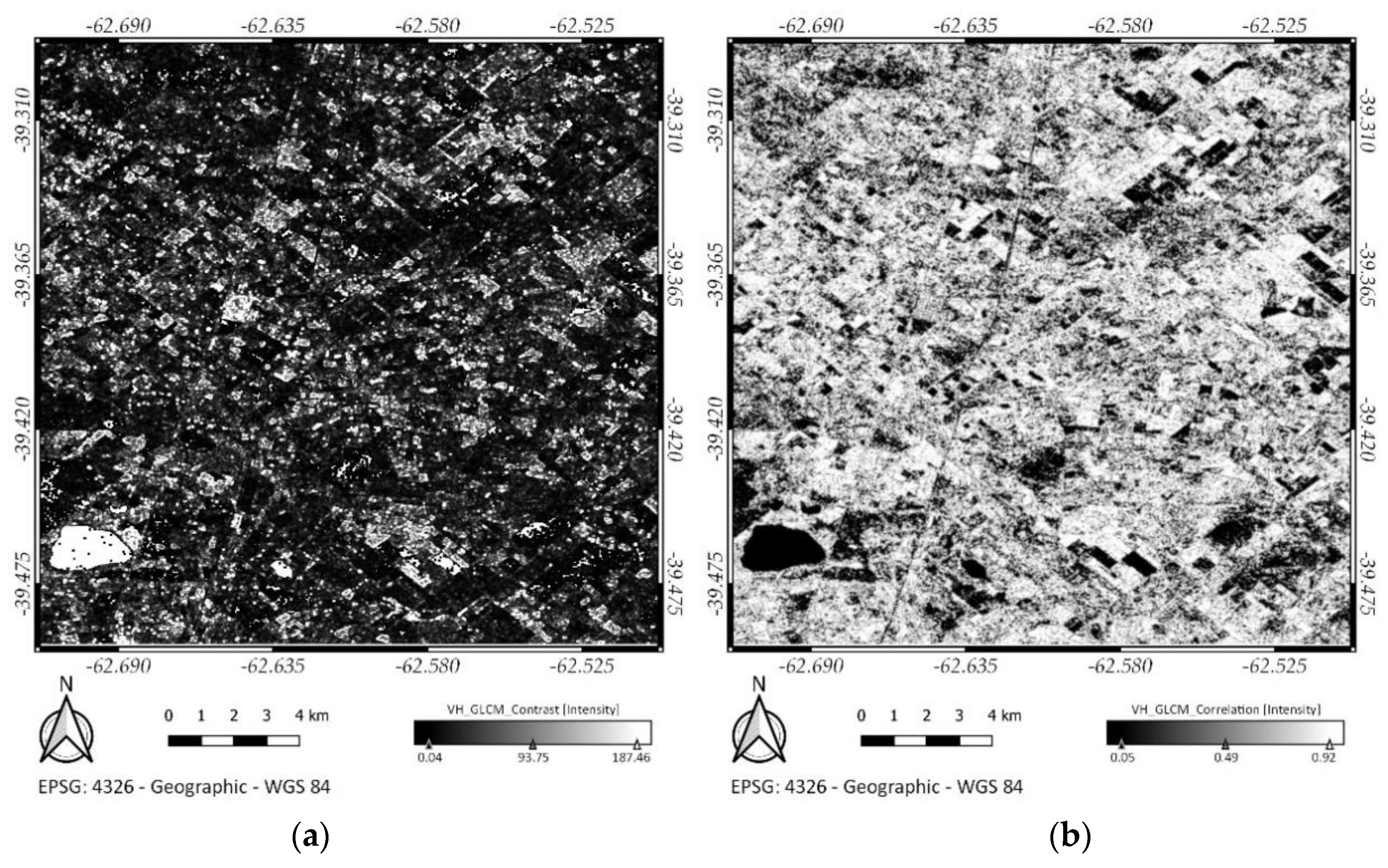
63]. We selected the following filter configuration parameters: Adaptive Neighbor Size = 15, Windows Size = 7 × 7, Number of Looks = 1. Finally, the GLCM texture analysis was performed on the time series stacks in both polarizations VV+VH. In order to discriminate between the S1 SAR images pixel spatial relationships, four GLCM texture measurements were obtained: correlation, contrast, entropy and variance. The employed GLCM module configuration parameters were the following: Windows Size = 9 × 9, Angle = All, Quantizer = Probabilistic Quantizer, Quantization Level = 32, Displacement = 4. We obtained eight S1 SAR texture time series stacks, four for VH polarization and four for VV polarization (see
Figure 7).
2.7. Sentinel-1 Object-Based Image Analysis Approach
To perform the onion and sunflower classification at object level (Object Based Image Analysis, OBIA), the pixel median value of the crop parcels was calculated. The image batch processing was done using the graphical modeler of the QGIS version 3.8.1 “Zanzibar”. The QGIS zonal statistics plugin allows the median value for each polygon of a vector-type layer to be calculated, taking a raster-type base layer as a reference. A new attribute corresponding to the median value of the SAR image pixels is added to each register of the field database (see
Figure 8). The process was repeated automatically for each SAR time series S1 processed image. A total of 300 new features were added to the GT database parcel registers: 60 for VH+VV polarizations and 240 for GLCM texture (correlation, contrast, entropy and variance). The temporal variation of the features allows onion crop parcels to be distinguished from sunflower ones. The 300 SAR processed features were used for training and testing the machine learning algorithms selected to perform the classification.
2.8. Classification Algorithms: RF and SVM
Once the object level classification database was created, two machine learning algorithms were evaluated, random forest and support vector machine, in order to carry out the supervised crop classification. RF is a classification binary tree based on the S1 SAR features (input) returning a classes label vector (output), where each branching node is split based on the values of an input column. The selected split criterion used to perform all the tests was GDI (Gini’s Diversity Index). The SVM configuration parameters are shown in
Table 3.
The box constraint configuration parameter aids in preventing overfitting (regularization); increasing the box constraint can lead to longer training times. The kernel scale ‘auto’ mode allows the software to use a heuristic procedure to select the scale value. Therefore, to reproduce the classification statistical results a random number seed was set before training the classifier. Standardize was set as ‘true’ indicating the software to center and scale each column of the predictor data (S1 SAR features) by the column mean and standard deviation, respectively. Different sets of SAR features were used to train the classification algorithms, each time obtaining different RF and SVM classification models and hyperparameter sets. As a complement, the combination (COMB) between SVM and RF using the maximum vote logic was assessed. A processing script was developed in MATLAB
® framework version R2015a. After the script execution an automatic test report was generated. A total of 15 tests was done using the S1 SAR dataset; the statistical OA and Kp values for the training and testing stages and the processing time for each machine learning algorithm were registered. The test reports also provide the classification confusion matrixes in the training and testing stages and the covariance matrix of the analyzed SAR features dataset. Regarding the test configuration parameters, it is also possible to consider or not the different crop classes present in the study site. The other crops are considered ‘image background’ and can be taken into account or not by modifying a Boolean variable value in the processing script. Likewise, it is possible to analyze the contribution of the principal components analysis to evaluate the effects of reducing the S1 SAR feature dataset size. The dataset was randomly split in two sets: 70% for the training dataset and 30% for the testing dataset. A summary of the processing chain implemented in this study is shown in
Figure 9.
Table 4 shows the configuration parameters of the 15 tests.
Tests can be grouped into four blocks according to the following description:
1st block: an analysis based on one date of the temporal series considering only VH+VV polarization features. Three onion crop representative cases were analyzed: the start of season, vegetation highest vigor and harvest. S1 SAR dataset dimension = 2 features.
2nd block: an analysis based on VH+VV temporal series, considering or not image background and PCA, four tests in total. S1 SAR dataset dimension = 60 features.
3rd block: an analysis based on SAR GLCM texture temporal series, considering or not image background and PCA, four tests in total. S1 SAR dataset dimension = 240 features.
4th block: an analysis based on the VH+VV+GLCM texture temporal series, considering or not image background and PCA, four tests in total. S1 SAR dataset dimension = 300 features.
3. Results
In this section the results of the 15 tests done for the evaluation of the capabilities of the temporal data series from S1 are presented. Two machine learning algorithms were evaluated: RF and SVM. As a complement, the results obtained from the combination between RF and SVM using the logic of the maximum vote are analyzed. In remote sensing mapping, the validity and reliability of classified maps are often decided on the basis of estimated OA and Kp [
64]. First, the values of OA and Kp obtained during the training and testing stages for the executed tests with only one scene of the temporal series are presented. In the next stage, the potential of the stack combination in both polarizations (VH+VV) and the GLCM of the texture products (contrast, correlation, entropy and variance) are analyzed.
3.1. BVCR Intensively Cultivated Parcels Identification Based on S1 SAR Time Series
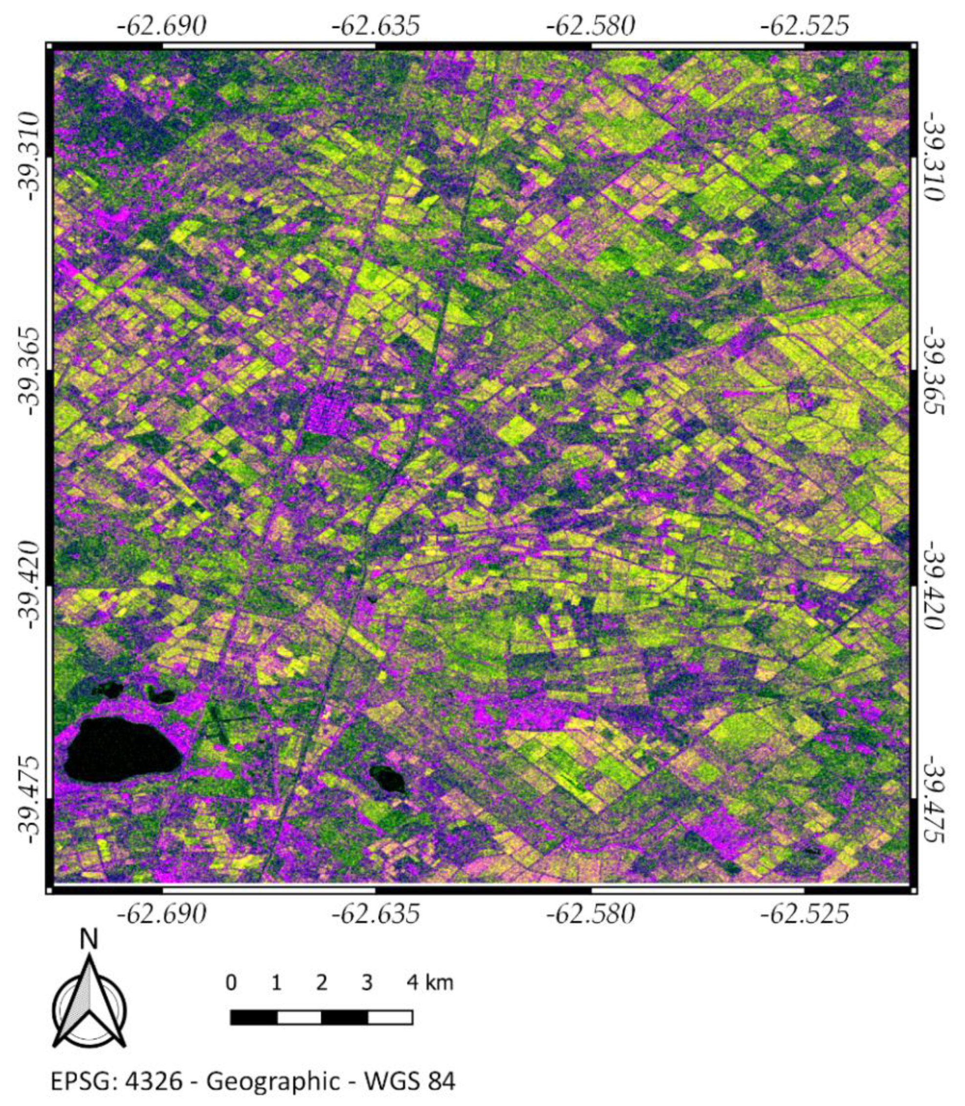
Once the S1 SAR images have been processed it is possible to build a raster map to identify the intensively cultivated crop parcels location in the study region of the irrigated valley of the Colorado River. Three new bands were obtained from the S1 VH polarization temporal series data. With the aid of GRASS version 7.6.1 and the “r.series” tool the temporal series maximum, minimun and the difference (maximun–minumum) was calculated. The “r.series” makes each map output pixel value a function of the several values assigned to the corresponding pixel in the temporal series raster map layers. The “min_raster” and “max_raster” methods generate new raster maps that hold the minimum/maximum value of the S1 VH polarization temporal series. There are different land cover types in the study site. While the VH backscattering coefficient remains constant throughout the time for scattering surfaces like asphalt, house roofs, water reservoirs and fields at rest, it varies widely for the surfaces of cultivated parcels. The difference between the S1 temporal series maximum and minimum products in VH polarization highlights the croplands in the BVCR raster map (see
Figure 10).
3.2. SAR OBIA Classification Based on One Date of the Temporal Series: VH+VV
In order to execute the tests, three scenes from the temporal series of the S1 SAR images on different dates were selected: October 11, 2017; January 15, 2018 and March 4, 2018. The dates correspond to the beginning of the planting season, the maximum vegetation vigor and the onion crop harvest for the 2017–2018 BVRC crop campaign. To perform the tests, the other crops (image background) in the study area were not taken into account. From the results registered in
Table 5, it can be seen that the highest OA (88.37%) and Kp (0.75) values during the validation stages are obtained when both polarizations of the S1 SAR image are used, corresponding to the maximum vigor of the vegetation for the onion crops (Test #2). When the classification is done with SAR images corresponding to the planting and harvest stages, the resulting Kp values obtained are low and the classification is poor according to the Monserud scale [
65], (Test #1 and #3).
3.3. SAR OBIA Classification Based on the Temporal Series: VH+VV
In this section, the results of the four tests performed on the stack VH+VV are presented. The temporal series of S1 SAR images has 30 scenes, which creates a 60-band stack when both polarizations are used. The influence of considering or not the different valley crops (image background) in the classification results and the contribution of narrowing the space of analysis with PCA was analyzed. Generally speaking, it can be seen in
Table 6 that the highest OA (95.35%) and Kp (0.89) values are obtained for the SVM algorithm using the stack VH+VV for the classification not considering other crops (Test #4). When other crops existing in the study area are taken into account, the statistical values of the classification are lower: OA (89.75%) and Kp (0.89) for SVM (Test #5). According to the Monserud scale, if the classification result implies that 0.55 < Kp < 0.70 then the classification is considered a good one. When the contribution of the PCA is considered, it can be concluded that the dimension of the space of analysis of the classification algorithms remains reduced by more than the 50% (Test #6 and #7). The stack reduction from 60 to 28 and 29 bands, respectively, implies that the processing times needed to train the classification algorithms are smaller, and conversely, the statistical values obtained are very good—OA (94.19%) and Kp (0.86)—when other crops are not considered during the process of differentiating onion from sunflower in the BVCR. When the PCA is applied and other crops in the study area are considered, the OA value is acceptable, but the Kp value (0.39) drives the classification to be considered as regular.
3.4. SAR OBIA Classification Based on the Temporal Series: GLCM
In this section, the results of the four tests performed on the stack of the GLCM texture (contrast, correlation, entropy and variance in both polarizations VH+VV) are presented. The temporal series of the S1 SAR images has 30 scenes, and 4 texture products for each polarization were obtained, which creates a 240-band stack. The influence of considering or not the different valley crops (image background) in the classification results and the contribution of narrowing the space of analysis with PCA was analyzed. It is possible to see in
Table 7 that the highest OA (93.02%) and Kp (0.86) were obtained for both SVM and RF algorithms, using the stack GLCM of the SAR texture for the classification without taking into account other crops (Test #8). When other crops existing in the study area are considered, the statistical values of the classification are slightly lower, OA (89.98%) and Kp (0.66) for SVM and OA (85.42%) and Kp (0.57) for RF in the validation stages (Test #9), which results in a good classification between onion and sunflower. The dimension of the space of analysis of the classification algorithms will be reduced by more than 62% when the principal components analysis is considered (Test #10 and #11). When other crops existing in the study area are not considered, very good statistical values are obtained: OA (88.37%) and Kp (0.76) for SVM. According to the Monserud scale, the classification is considered as very good when 0.70 < Kp < 0.85 (Test #10). When PCA is applied to the GLCM stack of SAR texture and other crops from the valley are considered, the Kp is 0.41 for RF and 0.29 for SVM, which means a regular or poor classification respectively (Test #11).
3.5. SAR OBIA Classification Based on the Temporal Series: VH+VV+GLCM
In this section the results of the four tests performed on the stack of the VH+VV polarizations and the texture GLCM stack are presented (
Table 8). A total of 300 derived bands of S1 SAR features for each crop parcel of onion or sunflower were applied. The influence of considering or not the different valley crops (image background) in the classification results and the contribution of narrowing the space of analysis with PCA were analyzed.
It is possible to see in
Table 8 that the highest OA (94.19%) and Kp (0.88) were obtained for SVM using the stack VH+VV+GLCM for the classification not taking into account other crops (Test #12). When other crops existing in the study area are considered, the statistical values of the classification are slightly lower, OA (89.98%) and Kp (0.66) for SVM and OA (86.33%) and Kp (0.57) for RF in the validation stages (Test #13), which results in a good classification between onion and sunflower in the BVCR. The dimension of the space of analysis of the classification algorithms are reduced by more than 70% when the principal components analysis is considered (Test #14 and #15). When other crops are not considered for the classification, the statistical values obtained are OA (89.53%) and Kp (0.78) for SVM and OA (84.88%) and Kp (0.69) for RF. When PCA is applied to the VH+VV+ GLCM stack of SAR texture and other crops from the valley are considered, the Kp is 0.36 for RF and 0.44 for SVM, which means a regular or poor classification respectively (Test #15).
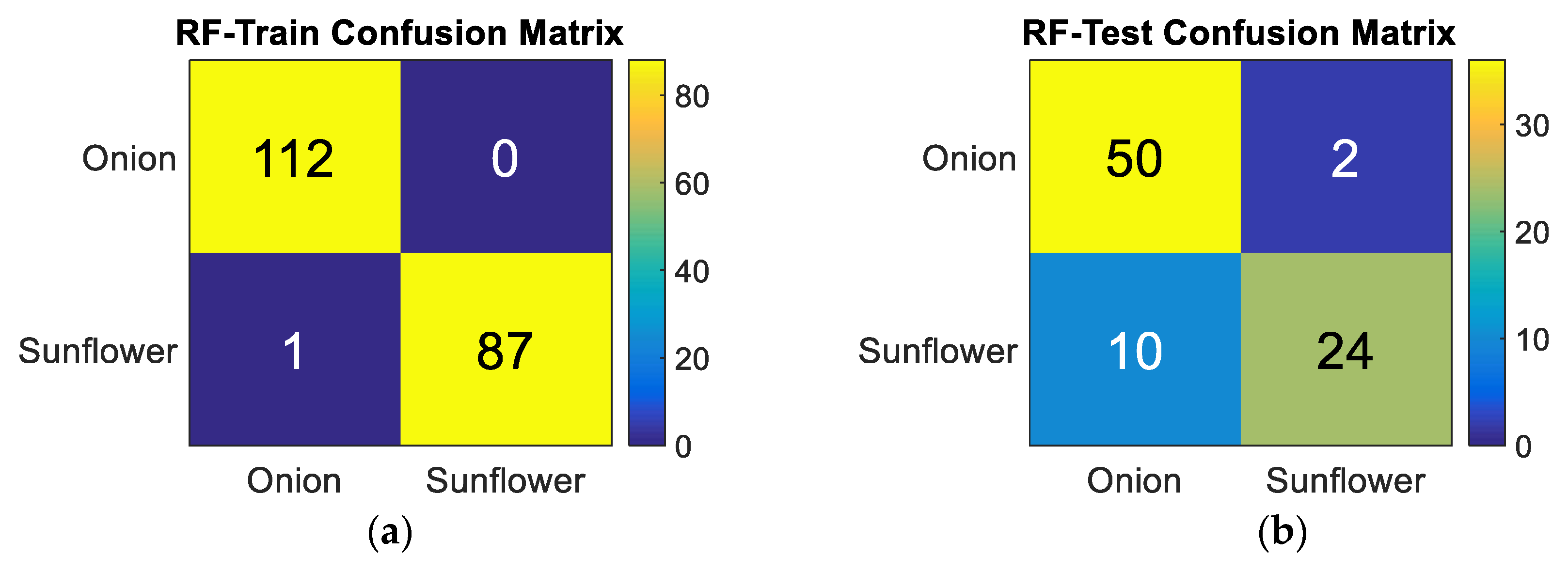
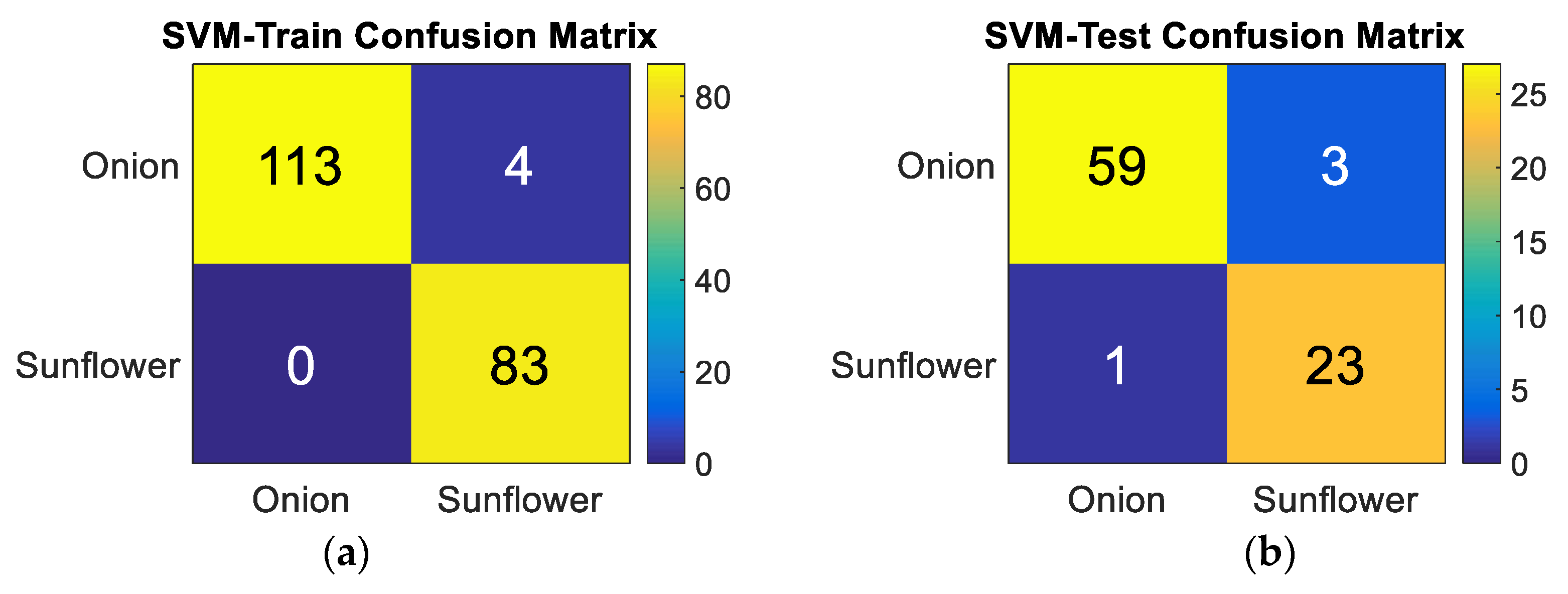
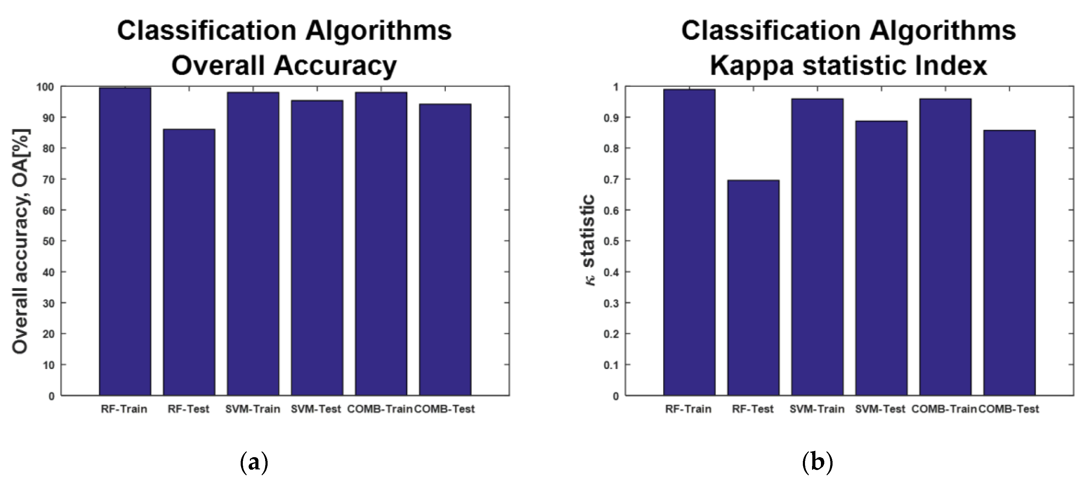
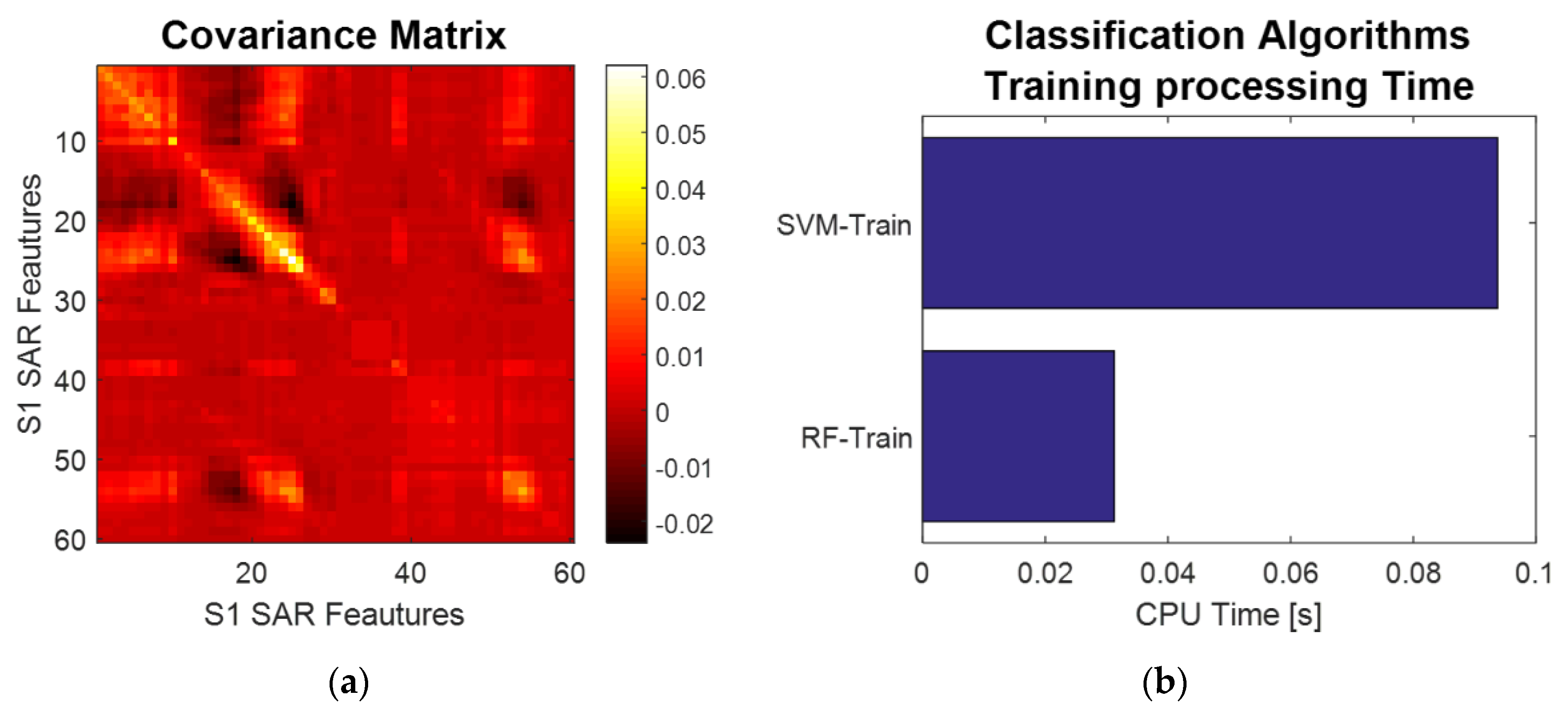
3.6. Test #4 Results: Analysis of the Temporal Series of Sentinel 1 SAR Data on the VH+VV Polarizations
In this section, the confusion matrix in the training and testing stages for the RF (
Figure 11) and SVM (
Figure 12) are presented, as well as a summary of the statistics for OA and Kp (
Figure 13), the covariance from the stack VH+VV and the processing times for each machine learning algorithm (
Figure 14) obtained for the Test #4.
4. Discussion
When performing the supervised classification based on a single date of the time series of the VH+VV stack of SAR images of S1, it was noted that the result is strongly related to the phenological stage of the crops found in the BVCR. When using S1 scenes corresponding to the beginning or the end of the onion growing season, the classification results are poor, and it is not feasible to differentiate sunflowers from onions. When the selected date corresponds to the maximum vigor of the onion crop (January 15, 2018), the SAR image of S1 in VH+VV polarization provides a “very good” ranking according to the Monserud scale, for RF as well as for SVM.
A crop classification on the BVCR considering the date of maximum vigor of vegetation based on S2 optical images was carried out in a previous study [
66]. S2 optical data allowed good classification results for the following algorithms: Linear Discriminant Analysis (LDA), RF, decision trees, and K-Nearest Neighbor (K-NN). Spectral information is an optimal study area for machine learning sorting algorithms; however, in certain regions it is not possible to use optical images because they may be affected by the clouds and weather conditions such as rain, fog, snow and dust. Therefore, the use of SAR images for classifying land cover in intensively cultivated agricultural regions becomes relevant.
Onion and sunflower crops phenological cycles are similar in the growing stage. When the onion is harvested, the sunflower remains standing; this condition can be noted in the VV backscatter coefficient temporal evolution. Due to the onion harvest, the bare soil produces a considerable contribution to the scattering superficial component, then the normalized gamma naught backscatter coefficient value in VV polarization increases. Meanwhile, the plant structure of the standing sunflower crops interacts with the SAR signal boosting the scattering volumetric contribution. This phenomenon can be noted in the VH polarization signal between the end of January and middle of February. In March, a large percentage of the onion crop has been harvested. Therefore, a significant predominance of the SAR backscattering signal in VV polarization can be found due to the bare soil scattering contribution.
When using the VH+VV stack of the S1 SAR image time series, the best statistical data are obtained from the classification test set. When other crops are not considered in the classification process, the following data is obtained: OA = 95.35%, Kp = 0.89; this result is categorized as excellent according to the Monserud scale. Analyzing the contribution of PCA to the classification process, we can notice that the worst condition is obtained for SVM when other crops besides onion and sunflower are considered. In general, the SVM results are better than those obtained from RF, except for the PCA with image background (considering other crops present in the study area).
The potential of the S1 SAR data time series in VH+VV polarizations to classify crops in the BVCR was shown by [
22]. The analyzed data correspond to the 2017-2018 BVCR crop campaign. Among other findings, it was highlighted that the onion and sunflower crops deserved special attention due to the particularities of their interaction with the SAR signal.
Using the GLCM time series data of correlation, contrast, entropy and variance in both polarizations, an excellent classification was obtained (OA = 94.19% and Kp= 0.88), according to the Monserud scale. Moreover, when other crops (image background) are considered, there is an improvement with respect to the VH+VV stack, an OA of 89.98% and a Kp 0.66 are obtained, statistics that rank the classification as “good”. This means that the SAR GLCM texture stack is slightly more robust than the VH+VV stack when analyzing the background contributions (see statistics in Results section).
For the first three test scenarios, the classification results are between good and excellent, whereas when PCA is applied and the image background is considered, the classification is regular. RF gets better classification results when using the GLCM stack instead of the VH+VV stack even when other crops are considered.
When studying the contribution of the analysis of principal components for both stacks (GLCM and VH+VV), better results are obtained for RF when other crops are not considered, whereas for SVM, the performance is lower for GLCM compared to VH+VV.
When applying PCA to the VH+VV stack and the image background is not considered, the stack dimension is reduced from 60 to 28 S1 SAR features, whereas when the image background is considered the S1 SAR stack dimension is reduced to 29 features. The PCA was performed by setting a total accumulated variance value of 95%. The software script allows modification of the variance value threshold, but sensitivity analysis of this parameter and its relationship with the S1 SAR stack size reduction is outside the scope of this investigation.
The GLCM S1 SAR stack dimension was also reduced carrying out the PCA. Considering or not the image background has a significant and diverse impact on the S1 SAR stack size reduction. When other crops are taken into account to train the SVM and RF algorithms, the training S1 stack size is reduced from 240 to 91 SAR features, whereas in those cases when only onion and sunflower are considered for the analysis, the final S1 SAR stack dimension after applying PCA is decreased to 75 features.
When other crops are considered to classify onion and sunflower, the GLCM+VH+VV stack provides the best solution for RF (OA = 86.33% and Kp = 0.57), and for SVM the results are the same as those obtained using the GLCM stack (OA = 89.98% and Kp = 0.66). The RF algorithm benefits from the use of the GLCM+VH+VV stack compared to the GLCM, whether the contribution of other crops is considered or not. Compared to the VH+VV stack, the GLCM+VH+VV stack produces no substantial ranking improvements. The dimension of the SAR features stack expands, from 60 to 300 bands, and so do the processing times for RF and SVM. If the contribution of PCA including other crops in the classification is analyzed, then there is an improvement when using the GLCM+VH+VV stack instead of the VH+VV stack. After applying PCA to the GLCM+VH+VV stack, the 300 derived bands of S1 SAR features are reduced to 87 and 72 when considering or not the image background, respectively.
The proposed classification method can be replicated in other large crop-dedicated regions of the world. Based on an S1 spatial resolution of 10 m, an object-based image analysis at lot level is appropriate to address the small size of crop parcels, especially in intensively cultivated areas of Europe, such as orchards in Valencia, Spain, Austria or Italy. Other challenges the method might face are the interclass crop adjacency and extreme weather conditions during the crop season, like snow, which can modify the dielectric constant of the scatter elements.
The number of ground truth samples must be considered for further analysis. The greater the number of samples to train the machine learning algorithm, the better the results of the classification statistics. Access to ground data might signify a key factor for an effective deployment of the classification method in other regions of the world.
Several radar signal incidence angles over the cropland regions might be analyzed in order to improve the robustness of the proposed classification method. The slope of the BVCR cultivated area was explained in
Section 2.4. The extremely soft slope of the Colorado River valley has a significant impact on the soil structure and composition, making it suitable for onion and sunflower crops, among others.
5. Conclusions
In this research study, the capacity of S1 C-band SAR time series imagery, considering the four seasons, has been analyzed to differentiate onion crop from sunflower crop, among others, using four less correlated GLCM texture measures: contrast, entropy, correlation and variance, as well as VH+VV polarizations time series. We obtained the textures measure from a GLCM using a 9 × 9 moving window, an aggregate orientation (θ) of all directions and a four-pixel displacement (δ) distance.
Among the crops present in the BVCR during the 2017-2018 BVCR crop campaign, the following classes are distinguished: onion, sunflower, squash, potato, alfalfa, winter cereals and forage pastures. Analysis of SAR data and their features at OBIA lot level shows an optimal strategy to counteract the effect of the residual and inherent speckle noise of the radar signal. The analysis carried out at polygon level was made possible through previous digitization and field data collection work (ground truth) performed in the BVCR during the 2017-2018 BVCR crop campaign. Within each lot it was possible to obtain the median value for each of the analyzed SAR characteristics: gamma naught VH, gamma naught VV, correlation, contrast, entropy and variance in both polarizations. Therefore, it was possible to reduce the speckle effect in each lot for each of the scenes of the time series analyzed.
The use of S1 high resolution C-band SAR data time series showed great potential for the classification of onion and sunflower crops in the BVCR, Buenos Aires Province, Argentina. Analysis of the VH+VV stack with the SVM algorithm delivered the best statistical classification results when the image background is not considered. Certainly, the GLCM texture analysis derived from the S1 SAR images is a valuable source of information for obtaining very good classification results. When differentiating sunflower from onion by considering other crops present in the BVCR, the GLCM stack represents the most robust dataset analyzed in this article. Considering that the GLCM+VH+VV stack does not provide significant advantages to the classification process when the image background is not considered and it produces increases in the size of the analysis space and in the processing times, then the improvement under certain test conditions can be considered as negligible.
Considering one date analysis, it was anticipated that the differentiation of onion and sunflower crops using S1 C-Band SAR data would be suitable at the end of January for the BVCR cultivated area, since the phenological differences between crops were greatest at this time. For example, the onion crop was in senescence and ready for harvest. On the other hand, the sunflower crop was in the maximum development stage.
The irrigation of the semi-arid region of the Colorado River valley has a significant impact on the nature of the soil scattering. The soil dielectric constant is strongly related to its moisture content and, to a lesser extent, the soil textural composition. The vegetation backscatter signal is also modified by the irrigation condition.
In general terms, applying PCA means a significant size reduction of the S1 SAR features stack. This remarkable stack dimension decrease shows the potential of the S1 SAR derived features time series information and its capability for monitoring the vegetation development throughout the complete phenological cycle of the crops.
We estimated the GLCM textures using a 9×9 moving window, considering the 10 m pixel resolution for S1 SAR images. However, different window sizes may influence both texture values and classification statistical results. The analysis of different window sizes, spatial orientations (θ) and displacement distances (δ) was not the focus of this study and may be a subject for further analyses.
This working methodology is applicable to other irrigated valleys in Argentina dedicated to intensive crops. There are also variables inherent to each lot, crop and agricultural producer that differ according to the study area. A line of research with so much potential leaves a large number of paths open, including the study of the sensitivity of the C-band SAR signal to differentiate irrigated from non-irrigated crops and the analysis of classification methods based on the merging of high resolution optical data and S1 radar data. Irrigation parameters, soil moisture, height of crops and phenological stage should be considered in future analyses.
We studied a total of 30 S1A images between April 14, 2017 and May 15, 2018. Studying the influence of the number of S1 images or their temporal correlation with the phenological state of crops is a goal for future studies. Along the same investigation line, analyzing the minimum number of SAR S1 features without degrading classification precision is a remaining line of work that should be addressed in future research studies. Future studies should incorporate the dynamics of the field due to changing crop seasons as well as winter and summer crop rotations.

 ,
, 


