Abstract
Statistical, data-driven methods are considered good alternatives to process-based models for the sub-national monitoring of cereal crop yields, since they can flexibly handle large datasets and can be calibrated simultaneously to different areas. Here, we assess the influence of several characteristics on the ability of these methods to forecast cereal yields at the local scale. We look at two diverse agro-climatic Italian regions and analyze the most relevant types of cereal crops produced (wheat, barley, maize and rice). Models of different complexity levels are built for all species by considering six meteorological and remote sensing indicators as candidate predictive variables. Yield data at three different spatial aggregation scales were retrieved from a comprehensive, farm-level dataset over the period 2001–2015. Overall, our results suggest the better predictability of summer crops compared to winter crops, irrespective of the model considered, reflecting a more intricate relationship among winter cereals, their physiology and weather patterns. At higher spatial resolutions, more sophisticated modelling techniques resting on feature selection from multiple indicators outperformed more parsimonious linear models. These gains, however, vanished as data were further aggregated spatially, with the predictive ability of all competing models converging at the agricultural district and province levels. Feature-selection models tended to elicit more satellite-based than meteorological indicators, with a preference for temperature indicators in summer crops, whereas variables describing the water content of the soil/plant were more often selected in winter crops. The selected features were, in general, equally distributed along the plant growing cycle.
1. Introduction
Timely and accurate yield forecasts of the most relevant cereal species are essential for the correct design, implementation and monitoring of major agricultural policies. In Europe, cereal yield forecasts contribute, for instance, to the cereal supply balance sheets of the European Union, which help to stabilize cereal prices and prevent market distortions within the European common market.
The spatial resolution of crop yield forecasts delivered by major operational forecasting systems is at most the regional or NUTS2 level (NUTS2 refers to regions belonging to the second level of the EU’s Nomenclature of Territorial Units for Statistics). Greater spatial detail of these forecasts would be desirable to adapt relevant agricultural policies to more specific target areas. However, the design of spatially resolved yield forecasting systems poses some challenges, which can be broadly classified into two categories: data-related and methodological. On the one hand, crop yield forecasting at the sub-regional level requires reliable and near real-time agro-climatic data, able to cover extensive areas with high temporal frequency. On the other hand, modelling methods are required to be flexible and computationally manageable tools.
The proliferation of agricultural farm-level yield datasets, the increase in the amount and resolution of Earth observation (EO) products and observed higher quality of meteorological gridded datasets help us to address data-related limitations. In recent years, the use of EO indicators has become very popular in agricultural applications. These products have been used to complement climate-based indicators in the calibration of crop models. [1] compared the accuracy of EO-based indicators against crop model indicators implemented in the crop growth monitoring system (CGMS) [2] for crop yield forecasting in Europe, and showed that EO-based biophysical indicators produced more accurate yield estimates in specific countries. The validity of EO products as yield predictors has been further confirmed with studies at the regional [3,4], and the sub-regional scale [5].
Current operational yield forecasting systems use either process-based methods, statistical (data-driven) methods [6], or a combination of them. For instance, in Europe, the approach of the MARS (Monitoring Agricultural Resources) Crop Yield Forecasting System (M-CYFS), developed and maintained by the European Commission’s Joint Research Centre (JRC), is based on gridded runs of the WOFOST (World Food Studies Simulation Model) process-based crop model and statistical methods [7]. Process-based crop models are highly parameterized and its calibration to large areas with diverse agro-climatic conditions is very difficult to achieve. In recent years, statistical methods have been gaining attraction, due to their simplicity and their ability to manage large amounts of data. These models have been applied, most often at the country or regional level, to study several issues: assess climate change impacts on yields [8,9,10]; identify factors determining crop productivity [11,12,13,14]; but also, as the basis for yield forecasting systems [15,16,17,18,19,20].
Statistical models are flexible enough to ingest large amounts of data and can be easily adapted to different agro-climatic areas. Their estimation, however, is often based on regression methods and can thus suffer from the known limitations and drawbacks of such models. For example, when the number of predictors is low, multiple linear regression models have proven to be successful [21,22]. Ref. [23] showed that linear models outperform in many cases more complex statistical models in explaining yield variability. However, when a high number of candidate explanatory variables are considered, OLS (ordinary least squares) estimation is often subject to overfitting problems, which weakens the prediction power of these approaches. For such cases, more sophisticated estimation techniques, such as ridge or lasso regressions are sometimes useful, especially when the number of variables is large compared to the number of data, and/or where these inputs are strongly correlated [24].
The aim of this study is to investigate the feasibility and performance of different local-scale statistical crop yield forecasting tools. Two diverse agro-climatic areas in Italy and four cereal species (wheat, barley, maize and rice) are considered. Forecasts derived from statistical models of different complexity levels under various spatial aggregation scales are compared.
2. Area of Study
Two diverse agro-climatic regions, the Apulia region, Puglia (abbreviated PG) in Italian, and the Po River Basin District (PRBD) are considered in this study (Figure 1). They are the main cereal-producing areas in Italy, accounting for more than two-thirds of national cereal production [25].
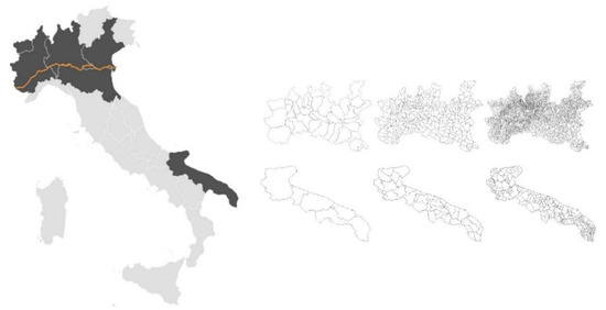
Figure 1.
Description of the studied area. An overview of the location of the two studied regions within Italy (left map), with Po river highlighted in orange. The three different spatial aggregation scales considered can be seen on the right-hand side panels: province (left), agricultural district (centre) and municipality (right).
PG is located in south-eastern Italy. About 70% of its surface, predominantly flat, is devoted to agriculture [26]. The most important agricultural land for production of cereals is situated in the central-northern zone, while olive trees and vineyards dominate the central and southern parts of the region. The climate is mainly of Mediterranean semi-arid type (Köppen: Csa), characterized by hot and dry summers and moderately cold and rainy winter seasons. Monthly precipitation ranges from about 30 mm/month in July, to 80 mm per month in November and December. Daily mean temperature seasonal cycles range from 7 °C in January to 25 °C in August [27]. Being surrounded by the seas, relative humidity in summer stays not lower than 50% [28].
The PRBD comprises five regions in northern Italy (Piedmont, Aosta Valley, Lombardy, Veneto and Emilia-Romagna), running from the Western Alps to the Adriatic Sea. The Po Valley has a warm oceanic climate (Köppen: Cfa), cool-humid with fog in winter and warm-moist in summer, with precipitation peaks in spring and autumn [29]. Mean daily temperature seasonality varies from just about zero degrees in winter to around 20 °C in summer [30]. On average, the precipitation over the Po basin is about 100 mm/month, with up to 50% difference among the seasonal peaks and the winter and summer dry period, and large interannual variability [29]. Climate in PRBD is strongly conditioned by orography. The Po valley, also known as Padan Plain, is structured as an extensive flatland, where the Alps protect the area from cold winds from north Europe, while the Apennines limit the mitigation action of the sea, favoring high levels of relative humidity throughout the year [31,32]. The relative humidity during summer is about 50%, similarly to PG [28]. The layout of the plain makes temperature variability over the year evenly distributed, in any point of the basin.
3. Materials and Methods
3.1. Yield Data
Farm-level, geo-referenced yield and surface data were retrieved from the Rete di Informazione Contabile Agricola (RICA) dataset, for a period covering the 2001–2015 growing seasons. RICA data is collected annually by the Italian Council for Agricultural Research and Economics (Consiglio per la Ricerca in agricoltura e l’analisi dell’Economia Agraria or CREA). CREA conducts field-level surveys providing data on a comprehensive list of agricultural and livestock variables from representative farms in Italy. The RICA-CREA dataset serves as the Italian input for the European Union’s Farm Accountancy Data Network (FADN; https://ec.europa.eu/agriculture/rica/), an instrument for evaluating the income of agricultural holdings and the impacts of the EU’s Common Agricultural Policy (CAP).
Four different cereal species (wheat, barley, maize and rice) are here analyzed. These four classes represent 97% of the total cereal production in the two studied regions. Most of the wheat in northern Italy is common wheat (around 80%), but durum wheat is also grown in the region (around the province of Parma), and its share within total wheat production keeps on rising. However, most of the durum wheat is grown in PG, the largest producing region in Europe. The cultivation of durum wheat in PG is overwhelmingly predominant, accounting for 92% of total cereal production in the region. Differences in the species and varieties grown in both regions, as well as diverse agro-climatic conditions, are reflected in the productivity of wheat farms, evidenced in Figure 2. Barley is also grown in PG and PRBD, but is relatively less important quantitatively, representing 5% and 4% of total regional cereal production, respectively. Maize and rice, mostly irrigated, are produced only in PRBD. These two crops are particularly relevant in the Po valley area and account for 82% and 98%, respectively, of the total national production. Except for wheat yields showing a slightly positive trend, cereal yields have remained stable over the study period in both regions (see Figures S1–S3 in the Supplementary Materials).
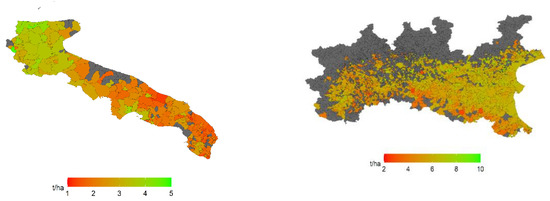
Figure 2.
Average wheat yields (tons/hectares) in Puglia (PG) (left) and the Po River Basin District (PRBD) (right), at the municipality level over the study period (2001–2015).
Despite RICA-CREA featuring a good spatial coverage of the two territories at the farm level (see Figures S4 and S5 in Supplementary Materials for a detailed description of the sampling frequency of each geographic area), there remain essentially two main reasons for data spatial aggregation: (1) RICA-CREA data show precise geo-reference information only after the year 2010. Prior to that year, only the municipality ascription of observed fields was provided; (2) survey-based data are usually subject to uncertainty associated to respondents inaccurately or falsely answering questions. Assuming a random bias in the responses, these uncertainties tend to mitigate when yield observations are spatially aggregated. Accordingly, three different scales of spatial aggregation are explored in this study: (i) municipality, (ii) Regione Agraria (agricultural district), and (iii) province (see right panels of Figure 1). For every season, crop and administrative unit considered, annual average cereal productivity was obtained as the total harvested product (tons) per aggregate unit of surface (hectare). A description of yield data at the three spatial aggregation scales studied can be found in Table 1.

Table 1.
Descriptive statistics of RICA-CREA yield data at the three spatial aggregation scales considered.
3.2. Yield Predictors
Several potential candidate predictors were considered. These indicators are broadly classified into two main families: meteorological and satellite-based indicators. Their sources, timespan and horizontal resolutions are described in Table 2. The selected indicators feature a native resolution below the size of the administrative units considered. Therefore, they were all trimmed and aggregated at the respective geographical unit of reference (municipality, agricultural district or province), using the 4th (2012) CORINE Land Cover inventory in Europe [33], and the corresponding boundaries maps. In particular, land cover class 2.1.1 (Non-irrigated arable land) was used for wheat, barley and maize, and class 2.1.3 (Rice fields) for rice. All variables (apart from precipitation, which was monthly cumulated) were averaged at the monthly scale. We distinguished between winter (wheat and barley) and summer crops (maize and rice). A homogenous growing season cycle was considered in both regions: a 9-month (October to June) growing cycle was assumed for winter crops and a 7-month (April to October) cycle for summer crops. Only monthly predictors belonging to the specified growing cycle periods were considered as candidate predictors.
Table 2.
Data sources and description of the weather and satellite-based indicators used in the construction of the analyzed statistical models.
3.2.1. Meteorological Variables
Temperature and precipitation time series were retrieved from the regional high-resolution (11 km) UERRA-Harmonie V1 reanalysis. This reanalysis was produced within the FP7 Uncertainties in Ensembles of Regional ReAnalysis UERRA project, with boundary conditions given by the global ERA-Interim reanalysis [34]. A complete description of the HARMONIE modelling system can be found in [35]. A drought stress index was derived from UERRA temperature and precipitation monthly time series. The Standardized Precipitation-Evapotranspiration Index (SPEI) [36] was calculated for each administrative unit (municipality, agricultural district and province), approximating potential evapotranspiration with the Thornthwaite equation [37]. The climatic water balance was computed on three different accumulation periods: 3, 6 and 9 months. Finally, SPEI values were obtained by standardizing monthly values of the climatic water balance over the analyzed period (2001–2015), using an empirical cumulative distribution function.
3.2.2. Remote Sensing Indicators
Three satellite-based indicators were considered in this analysis: the fraction of Absorbed Photosynthetically Active Radiation (fAPAR), Net Evapotranspiration (ET) and Land Surface Temperature (LST). These three indicators correlate well with crop yields [3,38,39,40], and are usually used as explanatory factors of yields in statistical models.
The fAPAR [41,42] is a spectral vegetation index quantifying the fraction of the solar radiation absorbed by live leaves for the photosynthesis activity. It refers only to the green and alive elements of the canopy. fAPAR data used in this study refer to version 2 of the data provided by [43]. LST (MOD11A2) [44] measures the radiative skin temperature of the land surface, including both vegetation and bare soil temperatures. It correlates but does not exactly matches surface air temperature. ET (MOD16A2) [45] summarizes part of the water cycle of the plant as the sum of evaporation and plant transpiration to the atmosphere. It is produced based on the logic of the Penman–Monteith equation [46], which includes inputs of daily meteorological reanalysis data along with remotely sensed data products, such as vegetation property dynamics, albedo, and land cover.
3.3. Statistical Models
We assessed the predictive ability of two different classes of models: parsimonious models, relying on a reduced number of predictors; and more complex, data-intensive models based on multiple indicators observed at different temporal scales. These families of models were applied to each region-crop combination under the three scales of spatial aggregation (municipality, agricultural district and province) considered.
Parsimonious models in this context are simple linear statistical models relying on a set of representative indicators within the growing season. In particular, a parsimonious model based on representative temperature (Temp) and precipitation (Prec) would read:
where yields of crop i relate linearly to monthly average temperature (Temp) and monthly cumulative precipitation (Prec), a constant term, a seasonal effect (Season) and a provincial fixed effect (NUTS3), while εi is a residual random error term. Yields come expressed in logarithms, which implicitly assumes that changes in the independent variables have the same percent impact on yields regardless of yield level. Equation (1) was estimated with OLS.
Parsimonious models were estimated for different candidate predictors, as described in Table 3 (rows 1–6). All possible monthly values over the hypothesized growing season were considered as candidate predictors. The final selected model was the one featuring lowest Root Mean Squared Error (RMSE). For instance, for the case of PG-Wheat (region-crop) and the family of models based on meteorological indicators (Model: Meteo), 9 different parsimonious models were estimated (a growing season of 9 months between October and June was assumed) and the model with greater predictive ability was retained. This estimation strategy was replicated for all the region-crop combinations and all the candidate models proposed.
Table 3.
Summary of the estimated models: model name identifier, indicators included, and estimation method used.
More complex models were also considered, on the premise that including more information potentially results in greater predictive accuracy. The following statistical model, based on the combination of meteorological and remote sensing indicators, was tested:
which differs from the parsimonious model described in Equation (1), in that here J = 6 indicators are included, represented by all their monthly values (Nk) over the respective growing cycle, with Nk equal to 9 and 7 for winter and summer crops, respectively. Since this approach implies working with an additional 54 predictors (number of predictors x number of months of the growing cycle) in the case of winter crops (42 additional predictors, if summer crops) on top of the seasonal and provincial fixed effects, a problem of overfitting could raise. We dealt with this problematic by resorting to regularization techniques [47,48]. These techniques are typically used to reduce the complexity of models in the presence of many, potentially correlated, features.
The most well know regularization alternatives are L1- and L2-type regularization. L1-type, also known as lasso (least absolute shrinkage and selection operator), adds “absolute value of magnitude” of coefficient as penalty term to the loss function. L2-type or ridge regularization adds “squared magnitude” of coefficient as penalty term to the loss function. The difference between these two techniques is that lasso performs variable selection by shrinking the less important feature’s coefficient to zero, thus, removing some features altogether and improving the sparsity of the model. In ridge regressions, all coefficients are shrunk towards zero, preventing from variable collinearity while controlling for overfitting. We used a specification that embeds the two types of penalties, known as elastic net [49]. Elastic net updates the general residual minimization function, by adding another term known as the regularization term.
Here, λ is the regularization tuning parameter and
where are not-penalised parameters and and are the L1-type and L2-type penalty terms, respectively. The hyperparameter λ controls the overall strength of the penalty and is chosen through cross-validation (note that if λ = 0, we are in the OLS case). The elastic net penalty is controlled by α, which modulates the influence of the lasso (α = 1) and ridge (α = 0) penalty terms. It is known that the ridge penalty shrinks the coefficients of correlated predictors towards each other, while the lasso tends to pick one of them and discard the others. The elastic net penalty mixes these two; if predictors are correlated in groups, an α = 0.5 tends to select the groups of indicators in or out together. Three different values of α were central in our analysis: α = 1 (lasso), α = 0.5 (elastic net) and α = 0 (ridge). Alternative estimations for α = 0.25, α = 0.75 and α = 1 − ε were also performed.
3.4. Estimation Strategy
As stated above, the hyperparameter λ for complex statistical models must be chosen through cross-validation. We implemented a cross-validation framework based on the construction of N = 1000 folds, resulting from randomly splitting the total sample into a training set (of size 2/3*N) and a validation set (1/3*N). The value of λ was chosen as the one which minimized the cross-validation error. Once λ was obtained, the root mean squared error (RMSE) of the predictions over the validation set was computed. These values were then averaged over folds. To preserve comparability, the constructed training-validation sets were also used for estimation and forecast accuracy on the parsimonious models.
In summary, we estimated a set of statistical models for each of the macro areas, available crops and spatial aggregation scales considered. For each of the 6 region-crop combinations and the three spatial aggregation scales proposed, 10 candidate models (7 parsimonious, 3 complex) were estimated, making a total of 10 × 6 × 3 = 180 estimated models. A full description of all these models can be found in Table 3.
4. Results and Discussion
An assessment of the predictive quality of the proposed models is presented and discussed in this section. Our analysis differentiated among cereal crops, as well as among different model complexity and spatial aggregation scales. By examining the outputs from feature selection models (lasso models), which (families of) indicators were preferred and the phase of the growing cycle of the plant of the selected indicators were also explored.
4.1. Model Accuracy by Cereal Species
Figure 3 and Figure 4 show the average root mean squared error (RMSE) of predictions within the cross-validation test datasets for all the proposed models. A summary of these findings by cereals species can be found in Table 4, where a region-crop, mean-adjusted average RMSE across specifications is computed. The ratio is obtained for each region-crop, where represents the average RMSE across all proposed models in a specific region-crop combination, and is the average yield within each specific region-crop combination.
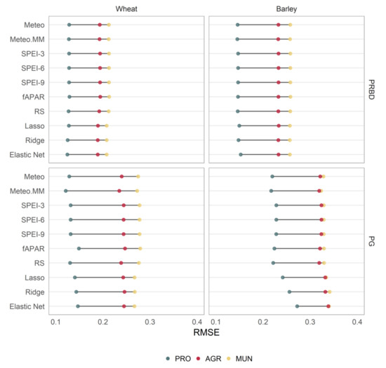
Figure 3.
Average RMSE of the estimated models for wheat (left) and barley (right) in PRBD (top) and PG (bottom), resulting from cross-validation estimation over N = 1000 training-validation folds. Three different levels of spatial aggregation were considered: municipality (MUN), agricultural district (AGR) and province level (PRO).
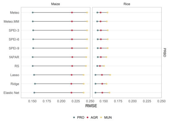
Figure 4.
Analogous to Figure 3, but for summer crops (maize and rice).
Table 4.
Average, mean-adjusted RMSE across all model specifications for the three spatial aggregation scale considered: municipality, agricultural district and province. A rank of the best predictable species at each administrative level is provided between parentheses.
Rice yield models showed, on average, the best forecasting performance at the municipality and agricultural district spatial aggregation scales. At the provincial scale, their relative accuracy decreased slightly in favor of maize and PRBD’s wheat yield models. Maize yield models followed in average performance, evidencing that summer crops tend to be more predictable than winter crops, possibly influenced by the smaller dispersion of their yields and their greater connection to heat stress. This better predictability has been early confirmed at the global level [14].
There existed notable differences in the forecasting accuracy of wheat yield models between regions, with wheat models in PRBD (where common wheat is predominant) behaving better than those in PG (durum wheat, mostly). Moreover, the ratio of these differences remained nearly constant over spatial aggregation scales. We attribute these differences to the heterogeneous performance of wheat farms within PG, where marked differences in the distribution of yields between North and South are observed (Figure 2). Our predictors failed to capture these differences, which suggest that they may lay on local characteristics, such as the type of soil (even though this variability may be partially captured by vegetation health remote sensing indicators), or in the amount and the intensity of use of various agro-management practices, such as the adjustment of sowing and harvest dates. The coexistence of common and durum wheat observations, especially in PRBD, could have also damaged the overall fit of wheat models.
Barley models featured the worst performance in both regions. Given the phenotypical similarities between wheat and barley and based on the findings of other studies (García-León et al. 2019), a similar performance between wheat and barley models was expected. We explain the relatively worse performance of barley models by the concurrence of two facts: first, barley is not a widespread crop in the studied regions, which results in a lesser amount of data being available; second, barley fields are sparse, especially in PG (Supplementary Figure S4), and their yields show very large dispersion, leading to less accurate estimations.
4.2. Differences across Spatial Scales
We observed generalized improvements in the performance of the proposed models after aggregating data to larger administrative units. Moreover, these improvements were homogenous across model specifications. When moving from the municipality to the agricultural district scale, an average of 10% RMSE reduction was observed for nearly all species. Gains when shifting to the provincial scale were strongly marked, but showed greater variability, with a decrease in RMSE ranging from 40% to 75%, depending on the crop species. These improvements in the overall predictability may be attributed to the observation of more stable yields at coarser spatial units, once data uncertainties, such as sampling errors and local factors, had been filtered out by spatial aggregation.
Interestingly, gains for rice yields were more moderate, with the RMSE of rice models being significantly lower at the municipality scale, compared to the rest of the crops. Rice is a case featuring several particularities: first, the production is highly concentrated in a relatively small geographic area (Supplementary Figure S5), making sampling errors at the municipality scale already low; second, rice fields are mostly irrigated and show a high degree of management, which probably decreases yield variability across spatial scales, because of a reduced impact of weather conditions; and third, there is a dedicated layer in CORINE to rice fields, making the extraction of weather and remote sensing indicators more precise.
4.3. Parsimonious Versus Complex Models
The performance of parsimonious models (Models 1 to 7 in Table 3) was compared against the performance of regularized models that rested on several predictors (Models 8 to 10 in Table 3). Also, within parsimonious models, different degrees of complexity were tested. Model performance differences were extracted from the analysis of Figure 3 and Figure 4.
Although it is difficult to generalize for all regions and species, Meteo models outperformed basic SPEI and fAPAR models. Some subtle gains were observed when extreme temperature values (Meteo.MM) instead of average values were accounted for. Even though simple models based on only fAPAR were not quite reliable, the addition of different sources of remote sensing indicators (RS) tended to improve their overall predictability and made them beat Meteo models in most cases.
Except for rice, regularized models, in any form, outperformed parsimonious models for all region-crop combinations at the municipality scale. These gains vanished as data was spatially aggregated, with all models at the agricultural district and province scales showing very similar performance. No significant differences were found among the three regularized methods considered. Different choices of the regularization parameter α were also explored, α = 0.25, α = 0.75 and α = 1 − ε (an alternative to lasso that removes any degeneracies and wild behaviour caused by extreme correlations), producing almost identical results (not shown).
Our results suggest that, when fine spatial resolution is sought, more complex models show better performance than any class of parsimonious models, based on a reduced number of either meteorological or remote sensing indicators. However, basic meteorological-based models could be as good as complex models to predict yield for large administrative units. Under coarse spatial resolutions, it was very hard to state which family of models performed best, as several models led to very similar performance levels. Given the opportunity cost of building more complex models, especially in terms of gathering and processing all the necessary data, it can be argued that simple parsimonious models are advisable for coarse spatial resolutions.
4.4. Nature of the Selected Predictors
By looking at the features selected by the lasso models, it can be inferred which indicator/family of indicators is more relevant to predict each crop in each region. Since looking directly at the size of the coefficients associated to each predictor can be misleading (even when predictors are standardized, so that they all showed the same mean and standard deviation prior to estimating the regressions), due to the collective constraint imposed on the size of the coefficients, it was opted to document the relative frequency of selected indicators along all the cross-validation simulations. These relative frequencies are shown for every model and spatial aggregation scale in Figure 5.
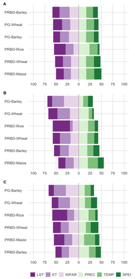
Figure 5.
Relative weight (%) of satellite-based indicators (purple-left) compared to meteorological indicators (green-right), within all selected features in lasso models at the province (A), agricultural district (B) and municipality level (C), for all the region-crop combinations.
A few messages can be extracted from the analysis of Figure 5. First, it was observed a general preference for the selection of satellite-based rather that meteorological predictors, regardless of the spatial detail considered. The relative weight of satellite indicators was always above 50% and was close to 75% in some cases. Second, indicators describing the water content of the soil/plant, such as ET and fAPAR, were selected more often in wheat and barley models, suggesting that moisture content is highly relevant for these two species. Third, in contrast to winter crops, temperature (both air temperature, temp, and ground temperature, LST) seems to be more relevant for the predictability of summer crops: maize and, especially, rice.
There was, however, considerable variation in the choice of selected input variables, and thus the results must be handled with caution. It was confirmed that the distribution of selected indicators was highly dependent on the strength of the regularization penalty, which relies on the value of the parameter λ. We experimented with different choices of λ, basically increasing the size of the penalty. It was observed that higher penalty values made the selection of indicators more stringent in detriment to the overall predictive quality of the model, causing in most cases that regularized models featured worse performance than parsimonious models. Feature selection should be further studied for other regions under different climatic conditions.
4.5. Timing of the Selected Predictors
We aggregated our candidate predictors at the monthly level, based on previous studies [10,20] and our own correlation analysis. Correlations between yields and predictors suggested that the optimal temporal aggregation window for indicators is the monthly level (as seen for wheat yields and fAPAR in Supplementary Figure S6). We assumed three different growing stages: early or tilling stage, mid or anthesis stage and late or grain filling stage. These stages were proportionally distributed over the growing cycles assumed for winter and summer crops.
Figure 6 describes the phases within the growing stage of the selected features by lasso. It was very hard to discern any clear time pattern within the selected indicators, as they were widespread over the entire growing cycle for most crops and spatial aggregation scales. Wheat in PG seemed to be more dependent on indicators belonging to the mid stage (January–March). More interestingly, most indicators of maize models were also drawn from the mid stage (June–August). The sign of the parameter estimates associated to the selected Temp and LST indicators was most of the time positive, suggesting that higher than average summer temperatures would decrease average maize yields. Given that it is inferred from the previous section that temperatures are relatively more relevant for this crop, it can be added here that summer temperatures are crucial to explain maize productivity.
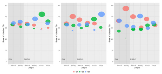
Figure 6.
Percentage of indicators belonging to each of the three growing stages (Q1, Q2 and Q3) of the plant, as derived from the selected features by lasso models under the three spatial aggregation scales considered: municipality (left), agricultural district (center) and province (right).
5. Conclusions
The predictive ability of several local-scale statistical models for Italian cereal yields was tested in this study. Summer crops showed relatively better predictability than winter crops, irrespective of the model considered. This may be partly explained by a more intricate relation between winter cereals and excess water scenarios, and because some winter species are subject to different physiological processes, such as vernalization, neither of which is well captured by our predictors. Differences in the fit of wheat models in both regions could also respond to common and durum wheat reacting differently to weather variations. More complex models based on feature selection outperformed parsimonious models, evidencing the gains of combining climate and satellite information. These gains, however, decreased as yield and predictors were spatially aggregated. Within feature selection models, a preference for satellite-based indicators was revealed, probably because their higher native resolution can better match local crop characteristics. We conclude, however, that feature selection from regularized models needs to be further explored, as it seems highly dependent on the total size of the regularization penalty. Finally, our results indicate that parsimonious models based on pure meteorological variables behave well in predicting cereal yields at coarse aggregation scales, but if finer levels of spatial detail are sought, combining information from different sources using; for instance, the regularization methods proposed in this study can improve the overall performance of crop yield forecasting tools.
Supplementary Materials
The following are available online at https://www.mdpi.com/2073-4395/10/6/809/s1, Figure S1:Wheat yields time series for various municipalities over the study period, Figure S2: Barley yields time series for various municipalities over the study period, Figure S3: Maize and rice yields time series for various municipalities in PRBD, Figure S4: Sampling coverage of RICA-CREA data at the municipality level in PG, Figure S5: Sampling coverage of RICA-CREA data at the province level in PRBD, Figure S6: Triangular correlation matrix between fAPAR and wheat yields over the growing season.
Author Contributions
Conceptualization, D.G.-L. and R.L.-L.; Data curation, D.G.-L., R.L.-L., A.T. and M.Z.; Formal analysis, D.G.-L., A.T. and M.Z.; Methodology, D.G.-L., R.L.-L., A.T. and M.Z.; Supervision, R.L.-L., A.T. and M.Z.; Visualization, D.G.-L.; Writing—Original draft, D.G.-L. All authors have read and agreed to the published version of the manuscript.
Funding
David García-León acknowledges financial support from the European Commission (H2020-MSCA-IF-2015) under REA grant agreement no. 705408.
Acknowledgments
We thank CREA for providing us with the farm-level agricultural data used in this study. David García-León would like to thank Giacinto Manfron for his assistance and support in the processing of the remote sensing data used in this study.
Conflicts of Interest
The authors declare no conflict of interest.
References
- Kowalik, W.; Dabrowska-Zielinska, K.; Meroni, M.; Raczka, T.U.; de Wit, A. Yield estimation using SPOT-VEGETATION products: A case study of wheat in European countries. Int. J. Appl. Earth Obs. Geoinfor. 2014, 32, 228–239. [Google Scholar] [CrossRef]
- Baruth, B.; Genovese, G.; Leo, O. CGMS Version 9.2—User Manual and Technical Documentation; EUR 22936 EN; OPOCE: Brussels, Belgium, 2007. [Google Scholar]
- López-Lozano, R.; Duveiller, G.; Seguini, L.; Meroni, M.; García-Condado, S.; Hooker, J.; Leo, O.; Baruth, B. Towards regional grain yield forecasting with 1 km-resolution EO biophysical products: Strengths and limitations at pan-European level. Agric. For. Meteorol. 2015, 206, 12–32. [Google Scholar] [CrossRef]
- Zampieri, M.; Carmona García, G.; Dentener, F.; Gumma, M.K.; Salamon, P.; Seguini, L.; Toreti, A. Surface Freshwater Limitation Explains Worst Rice Production Anomaly in India in 2002. Remote Sens. 2018, 10, 244. [Google Scholar] [CrossRef]
- García-León, D.; Contreras, S.; Hunink, J. Comparison of meteorological and satellite-based drought indices as yield predictors of Spanish cereals. Agric. Water Manag. 2019, 213, 388–396. [Google Scholar] [CrossRef]
- Basso, B.; Cammarano, D.; Carfagna, E. Review of crop yield forecasting methods and early warning systems. In Proceedings of the First Meeting of the Scientific Advisory Committee of the Global Strategy to Improve Agricultural and Rural Statistics, FAO Headquarters, Rome, Italy, 18–19 July 2013; pp. 18–19. [Google Scholar]
- Van Diepen, C.A.; Boogaard, H.L.; Supit, I.; LAZAR, C.; Orlandi, S.; van der Goot, E.; Schapendonk, A. Methodology of the MARS crop yield forecasting system. In Volume 2 Agrometeorological Data Collection, Processing and Analysis; Office for Official Publications of the European Communities: Luxembourg, 2004. [Google Scholar]
- Schlenker, W.; Roberts, M.J. Nonlinear temperature effects indicate severe damages to U.S. crop yields under climate change. Proc. Natl. Acad. Sci. USA 2009, 106, 15594–15598. [Google Scholar] [CrossRef] [PubMed]
- Lobell, D.B.; Burke, M.B. On the use of statistical models to predict crop yield responses to climate change. Agric. For. Meteorol. 2010, 150, 1443–1452. [Google Scholar] [CrossRef]
- Sharif, B.; Makowski, D.; Plauborg, F.; Olesen, J.E. Comparison of regression techniques to predict response of oilseed rape yield to variation in climatic conditions in Denmark. Eur. J. Agron. 2017, 82, 11–20. [Google Scholar] [CrossRef]
- Tack, J.; Barkley, A.; Nalley, L.L. Effect of warming temperatures on U.S. wheat yields. Proc. Natl. Acad. Sci. USA 2015, 112, 6931–6936. [Google Scholar] [CrossRef] [PubMed]
- Ben-Ari, T.; Adrian, J.; Klein, T.; Calanca, P.; Van der Velde, M.; Makowski, D. Identifying indicators for extreme wheat and maize yield losses. Agric. For. Meteorol. 2016, 220, 130–140. [Google Scholar] [CrossRef]
- Ceglar, A.; Toreti, A.; Lecerf, R.; van der Velde, M.; Dentener, F. Impact of meteorological drivers on regional inter-annual crop yield variability in France. Agric. For. Meteorol. 2016, 216, 58–67. [Google Scholar] [CrossRef]
- Zampieri, M.; Ceglar, A.; Dentener, F.; Toreti, A. Wheat yield loss attributable to heat waves, drought and water excess at the global, national and subnational scales. Environ. Res. Lett. 2017, 12, 064008. [Google Scholar] [CrossRef]
- De Wit, A.; Baruth, B.; Boogaard, H.; van Diepen, K.; van Kraalingen, D.; Micale, F.; te Roller, J.; Supit, I.; van den Wijngaart, R. Using ERA-INTERIM for regional crop yield forecasting in Europe. Clim. Res. 2010, 44, 41–53. [Google Scholar] [CrossRef]
- Peltonen-Sainio, P.; Jauhiainen, L.; Trnka, M.; Olesen, J.E.; Calanca, P.; Eckersten, H.; Eitzinger, J.; Gobin, A.; Kersebaum, K.C.; Kozyra, J.; et al. Coincidence of variation in yield and climate in Europe. Agric. Ecosyst. Environ. 2010, 139, 483–489. [Google Scholar] [CrossRef]
- Bannayan, M.; Sanjani, S. Weather conditions associated with irrigated crops in an arid and semiarid environment. Agric. For. Meteorol. 2011, 151, 1589–1598. [Google Scholar] [CrossRef]
- Gouache, D.; Bouchon, A.-S.; Jouanneau, E.; Le Bris, X. Agrometeorological analysis and prediction of wheat yield at the departmental level in France. Agric. For. Meteorol. 2015, 209–210, 1–10. [Google Scholar] [CrossRef]
- Schauberger, B.; Gornott, C.; Wechsung, F. Global evaluation of a semi-empirical model for yield anomalies and application to within-season yield forecasting. Glob. Chang. Biol. 2017, 23, 4750–4764. [Google Scholar] [CrossRef] [PubMed]
- Lecerf, R.; Ceglar, A.; López-Lozano, R.; Van der Velde, M.; Baruth, B. Assessing the information in crop model and meteorological indicators to forecast crop yield over Europe. Agric. Syst. 2019, 168, 191–202. [Google Scholar] [CrossRef]
- Quiring, S.M.; Papakryiaokou, T.N. An evaluation of agricultural drought indices for the Canadian prairies. Agric. For. Meteorol. 2003, 168, 49–62. [Google Scholar] [CrossRef]
- Bachmair, S.; Tanguy, M.; Hannaford, J.; Stahl, K. How well do meteorological indicators represent agricultural and forest drought across Europe? Environ. Res. Lett. 2018, 13, 034042. [Google Scholar] [CrossRef]
- Michel, L.; Makowski, D. Comparison of statistical models for analyzing wheat yield time series. PLoS ONE 2013, 8, e78615. [Google Scholar] [CrossRef]
- Wallach, D.; Makowski, D.; Jones, J.; Brun, F. Working with Dynamic Crop Models—Methods, Tools and Examples for Agriculture and Environment; Academic Press: Cambridge, MA, USA, 2014. [Google Scholar]
- ISTAT—Istituto Nazionale di Statistica. Superficie (Ettari) e Produzione (Quintali): Cereali. Dettaglio per Regione. (Surface and Production of Cereals. Breakdown by Regions). 2015. Available online: http://agri.istat.it/sag_is_pdwout/jsp/consultazioneDati.jsp (accessed on 25 January 2019). (In Italian).
- Steduto, P.; Todorovic, M. The Agro-ecological characterisation of Apulia region (Italy): Methodology and experience. In Soil Resources of Southern and Eastern Mediterranean Countries; Options Méditerranéennes: Série B. Etudes et Recherches; n. 34; Zdruli, P., Steduto, P., Lacirignola, C., Montanarella, L., Eds.; CIHEAM: Bari, Italy, 2001; pp. 143–158. [Google Scholar]
- Pizzigalli, C.; Palatella, L.; Zampieri, M.; Liobello, P.; Miglietta, M.M.; Paradisi, P. Dynamical and Statistical Downscaling of Precipitation and Temperature in a Mediterranean Area. Ital. J. Agron. 2012, 7, e2. [Google Scholar] [CrossRef]
- Diffenbaugh, N.S.; Pal, J.S.; Giorgi, F.; Gao, X. Heat stress intensification in the Mediterranean climate change hotspot. Geophys. Res. Lett. 2007, 34. [Google Scholar] [CrossRef]
- Zampieri, M.; Scoccimarro, E.; Gualdi, S.; Navarra, A. Observed shift towards earlier spring discharge in the main Alpine rivers. Sci. Total Environ. 2015, 503–504, 222–232. [Google Scholar] [CrossRef]
- Zampieri, M.; Giorgi, F.; Lionello, P.; Nikulin, G. Regional climate change in the Northern Adriatic. Phys. Chem. Earth 2012, 40–41, 32–46. [Google Scholar] [CrossRef]
- Po River Basin Authority. Caratteristiche del Bacino del Fiume Po e Primo Esame dell’ Impatto Ambientale Delle Attivitá Umane Sulle Risorse Idriche (Characteristics of Po River Catchment and First Investigation of the Impact of Human Activities on Water Resources). 2006. Available online: http://www.adbpo.it/download/bacino_Po/AdbPo_Caratteristiche-bacino-Po_2006.pdf/ (accessed on 27 January 2019). (In Italian).
- Vitali, A.; Segnalini, M.; Esposito, S.; Lacetera, N.; Nardone, A.; Bernabucci, U. The changes of climate may threat the production of Grana Padano cheese: Past, recent and future scenarios. Ital. J. Anim. Sci. 2018, 18, 922–933. [Google Scholar] [CrossRef]
- Buttner, G.; Feranec, J.; Jaffrain, G.; Mari, L.; Maucha, G.; Soukup, T. The CORINE land cover project. EARSel E Proc. 2004, 3, 331–346. [Google Scholar]
- Dee, D.P.; Uppala, S.M.; Simmons, A.J.; Berrisford, P.; Poli, P.; Kobayashi, S.; Andrae, U.; Balmaseda, M.A.; Balsamo, G.; Bauer, P.; et al. The ERA-Interim reanalysis: Configuration and performance of the data assimilation system. Q. J. R. Meteorol. Soc. 2011, 137, 553–597. [Google Scholar] [CrossRef]
- Ridal, M.; Olsson, E.; Unden, P.; Zimmermann, K.; Ohlsson, A. HARMONIE Reanalysis Report of Results and Dataset; UERRA Deliverable D2.7. 2017. Available online: http://uerra.eu/component/dpattachments (accessed on 5 June 2020).
- Vicente-Serrano, S.M.; Beguería, S.; López-Moreno, J.I. A Multi-scalar drought index sensitive to global warming: The Standardized Precipitation Evapotranspiration Index—SPEI. J. Clim. 2010, 23, 1696–1718. [Google Scholar] [CrossRef]
- Thornthwaite, C.W. An approach toward a rational classification of climate. Geogr. Rev. 1948, 38, 55–94. [Google Scholar] [CrossRef]
- Siebert, S.; Ewert, F.; Rezaei, E.E.; Kage, H.; Graß, R. Impact of heat stress on crop yield—On the importance of considering canopy temperature. Environ. Res. Lett. 2014, 9, 044012. [Google Scholar] [CrossRef]
- WMO; GWP. Handbook of Drought Indicators and Indices. Integrated Drought Management Tools and Guidelines; Svoboda, M., Fuchs, B.A., Eds.; World Meteorological Organization: Geneva, Switzerland; Global Water Partnership: Stockholm, Sweden, 2016. [Google Scholar]
- Bokusheva, R.; Kogan, F.; Vitkovskaya, I.; Conradt, S.; Batyrbayeva, M. Satellite-based vegetation health indices as a criteria for insuring against drought-related yield losses. Agric. For. Meteorol. 2016, 220, 200–206. [Google Scholar] [CrossRef]
- Myneni, R.B.; Hoffman, S.; Knyazikhin, Y.; Privette, J.L.; Glassy, J.; Tian, Y.; Wang, Y.; Song, X.; Zhang, Y.; Smith, G.R.; et al. Global products of vegetation leaf area and fraction absorbed PAR from year one of MODIS data. Remote Sens. Environ. 2002, 83, 214–231. [Google Scholar] [CrossRef]
- Baret, F.; Weiss, M.; Lacaze, R.; Camacho, F.; Makhmara, H.; Pacholczyk, P.; Smets, B. GEOV1: LAI, FAPAR Essential Climate Variables and FCover global times series capitalizing over existing products. Part 1: Principles of development and production. Remote Sens. Environ. 2013, 137, 299–309. [Google Scholar] [CrossRef]
- Copernicus Global Land Service. Fraction of Absorbed Photosynthetically Active Radiation, Sensor SPOT-VGT, PROBA-V, Product Version 2 [Data Set]. 2017. Available online: https://land.copernicus.eu/global/products/fapar (accessed on 1 November 2017).
- Wan, Z.; Hook, S.; Hulley, G. MOD11A2 MODIS/Terra Land Surface Temperature/Emissivity 8-Day L3 Global 1 km SIN Grid V006 [Data Set]. NASA EOSDIS LP DAAC. 2015. Available online: http://dx.doi.org/10.5067/MODIS/MOD11A2.006 (accessed on 1 November 2017).
- Running, S.; Mu, Q.; Zhao, M. MOD16A2 MODIS/Terra Net Evapotranspiration 8-Day L4 Global 500 m SIN Grid V006 [Data Set]. NASA EOSDIS Land Processes DAAC. 2017. Available online: http://dx.doi.org/10.5067/MODIS/MOD16A2.006 (accessed on 1 November 2017).
- Allen, R.G.; Pereira, L.S.; Raes, D.; Smith, M. Crop Evapotranspiration: Guidelines for Computing Crop Requirements; Irrigation and Drainage Paper 56; FAO: Rome, Italy, 1998. [Google Scholar]
- Tibshirani, R. Regression shrinkage and selection via the Lasso. J. R. Stat. Soc. Ser. B Stat. Methodol. 1996, 58, 267–288. [Google Scholar] [CrossRef]
- Efron, B.; Hastie, T.; Johnstone, I.; Tibshirani, R. Least angle regression. Ann. Stat. 2004, 32, 407–451. [Google Scholar]
- Hastie, T.; Tibshirani, R.; Friedman, J.H. The Elements of Statistical Learning: Data Mining, Inference and Prediction, 2nd ed.; Springer: New York, NY, USA, 2009. [Google Scholar]
© 2020 by the authors. Licensee MDPI, Basel, Switzerland. This article is an open access article distributed under the terms and conditions of the Creative Commons Attribution (CC BY) license (http://creativecommons.org/licenses/by/4.0/).