Article

Assessing Soil Key Fertility Attributes Using a Portable X-ray Fluorescence: A Simple Method to Overcome Matrix Effect

by
Tiago Rodrigues Tavares
1,2,
Abdul Mounem Mouazen
2,
Elton Eduardo Novais Alves
3,
Felipe Rodrigues dos Santos
4,
Fábio Luiz Melquiades
4,
Hudson Wallace Pereira de Carvalho
5 and
José Paulo Molin
1,*
1
Laboratory of Precision Agriculture (LAP), Department of Biosystems Engineering, “Luiz de Queiroz” College of Agriculture (ESALQ), University of São Paulo (USP), Piracicaba 13418900, São Paulo, Brazil
2
Precision Soil and Crop Engineering Group (Precision SCoRing), Department of Environment, Faculty of Bioscience Engineering, Ghent University, Coupure Links 653, Blok B, 1st Floor, 9000 Gent, Belgium
3
Laboratory of 14 Carbon (LC14), Center for Nuclear Energy in Agriculture (CENA), University of São Paulo (USP), Piracicaba 13416000, São Paulo, Brazil
4
Laboratory of Applied Nuclear Physics (LFNA), Department of Physics, Londrina State University (UEL), Londrina 86057970, Paraná, Brazil
5
Laboratory of Nuclear Instrumentation (LIN), Center for Nuclear Energy in Agriculture (CENA), University of São Paulo (USP), Piracicaba 13416000, São Paulo, Brazil
*
Author to whom correspondence should be addressed.
Agronomy 2020, 10(6), 787; https://doi.org/10.3390/agronomy10060787
Submission received: 28 April 2020 / Revised: 24 May 2020 / Accepted: 26 May 2020 / Published: 1 June 2020
(This article belongs to the Special Issue Precision Agriculture for Sustainability)

Abstract

:
The matrix effect is one of the challenges to be overcome for a successful analysis of soil samples using X-ray fluorescence (XRF) sensors. This work aimed at evaluation of a simple modeling approach consisted of Compton normalization (CN) and multivariate regressions (e.g., multiple linear regressions (MLR) and partial least squares regression (PLSR)) to overcome the soil matrix effect, and subsequently improve the prediction accuracy of key soil fertility attributes. A portable XRF was used for analyzing 102 soil samples collected from two agricultural fields with contrasting soil matrices. Using the intensity of emission lines as input, preprocessing methods included with and without the CN. Univariate regression models for the prediction of clay, cation exchange capacity (CEC), and exchangeable (ex-) K and Ca were compared with the corresponding MLR models to assess matrix effect mitigation. The MLR and PLSR models improved the prediction results of the univariate models for both preprocessing methods, proving to be promising strategies for mitigating the matrix effect. In turn, the CN also mitigated part of the matrix effect for ex-K, ex-Ca, and CEC predictions, by improving the predictive performance of these elements when used in univariate and multivariate models. The CN has not improved the prediction accuracy of clay. The prediction performances obtained using MLR and PLSR were comparable for all evaluated attributes. The combined use of CN with multivariate regressions (MLR or PLSR) achieved excellent prediction results for CEC (R2 = 0.87), ex-K (R2 ≥ 0.94), and ex-Ca (R2 ≥ 0.96), whereas clay predictions were comparable with and without CN (0.89 ≤ R2 ≤ 0.92). We suggest using multivariate regressions (MLR or PLSR) combined with the CN to remove the soil matrix effects and consequently result in optimal prediction results of the studied key soil fertility attributes. The prediction performance observed for this solution showed comparable results to the approach based on the preprogrammed measurement package tested (Geo Exploration package, Bruker AXS, Madison, WI, USA).

1. Introduction

An accurate characterization of spatiotemporal variation of soil key fertility attributes is important for the successful implementation of precision agriculture (PA) [1]. However, the classical mapping methods based on soil sampling followed by laboratory soil analysis is not a practical and cost-effective approach, especially because a high spatial density sampling is required for a reliable characterization [2,3]. The recent development of proximal soil sensing technologies enabled a fast, cost-effective, easy-to-use, and environmentally friendly way for soil attributes mapping [4,5,6]. These sensing techniques overcome the disadvantage of traditional soil sampling and test methods [3,7].
X-ray fluorescence (XRF) spectrometry is a well-established bulk analytical technique to assess the total content of several chemical elements in many different types of samples. Besides total elemental quantification, reports demonstrated XRF as a promising sensing technology for soil fertility assessment in the PA context [8,9]. Benchtop and portable XRF equipment are used for direct analysis of solid samples, with minimal or no sample preparation [10]. There is an increasing interest in this technique in recent years due to advances in engineering that have allowed the construction of robust equipment, with reduced weight and size; hence, compatible with in situ analyses [11]. Besides, some recent works have shown promising results for the prediction of organic matter (OM) [12], chemical attributes (base saturation (V), cation exchange capacity (CEC), and pH) [9,13,14,15,16,17], exchangeable (ex-) nutrients (ex-P, ex-K, ex-Ca, and ex-Mg) [10,16,18] and soil texture [19,20,21]. However, the application of XRF sensors as a practical tool for fertility analysis on agricultural soils is still at its early stages of development and further research are needed [18,21], particularly for developing transparent procedures and protocols for XRF data acquisition and modeling, as discussed by Tavares et al. [22].
The majority of studies evaluating the performance of XRF sensors for practical soil analysis have used preprogrammed measurement packages (e.g., Soil Mode (Innov-X Systems, Inc., Waltham, MA, USA) and Geo Exploration (Bruker AXS, Madison, WI, EUA)) [13,14,16,17,18,19,23,24,25]. These packages have pre-established instrumental conditions for data acquisition (e.g., X-ray tube operational settings, scanning time, etc.) and spectral analysis (e.g., matrix effects correction, quantification based on the fundamental parameter method, etc.), resulting in total elemental content of the soil sample. These packages also implement solutions to mitigate the matrix effect, facilitating the use of XRF sensors by nonexpert users [26]. However, preprogrammed measurement packages are associated with a pre-established scanning time (e.g., generally between: 60 and 90 s) [27], which is a constraint for the development of proximal soil sensing (PSS) applications that require rapid analysis (e.g., online analysis using mobile platforms). In this regard, new solutions for XRF data acquisition and analysis, avoiding the use of preprogrammed measurement packages and using the direct information of XRF spectra, should be developed to expand the use of XRF sensors in the PSS context.
Due to the heterogeneous and complex nature, XRF analysis of soils is prone to matrix effects [26], which refer to the influences of the different soil constituents in promoting absorptions or enhancements of emission lines of a given analyte under consideration [28]. When the matrix effects vary significantly between different samples that compose a dataset it must be corrected to achieve accurate predictive models [29]. A simple and widespread method for matrix effect correction is the Compton normalization (CN), which consists of using the Compton peak to normalize the analyte emission line [30]. As the Compton peak intensity is inversely proportional to the average atomic mass of a sample, it may play an important role in discriminating between different sample sets each having similar matrices. Another alternative solution for mitigating the matrix effect is the use of multivariate statistics approaches (e.g., multiple linear regression (MLR) or partial least squares regression (PLSR)) with emission lines intensities and scattering peaks used as input X-variables [31]. However, models should be established with soil samples having similar matrices to ensure the best prediction performance. Combining CN with multivariate statistics could be the ideal transparent solution to overcome the matrix effects and achieve the best prediction accuracy. To the best of our knowledge, no previous studies have attempted to evaluate solutions for matrix effect mitigation by combining CN and multivariate modeling approaches. Therefore, this work aimed at the evaluation of the combined effects of CN and multivariate regressions (MLR and PLSR) on the attenuation of the soil matrix effects (using data of two fields with considerable matrix effect) and consequently improve the prediction accuracy of key soil fertility attributes (clay, CEC, ex-K, and ex-Ca). In addition, the prediction performance achieved with the proposed solutions was also compared to that obtained from the Geo Exploration package (Bruker AXS, Madison, WI, EUA), a preprogrammed measurement package.

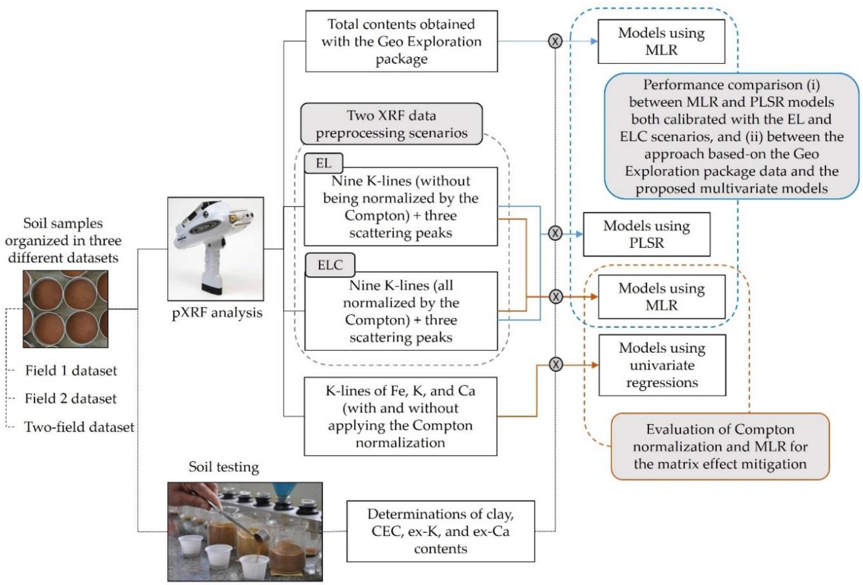
2. Materials and Methods

The different methodology steps followed in this work to fulfill the paper aim are shown by the block diagram of Figure 1. These steps can be divided into main tasks of soil sampling, XRF and laboratory chemical analyses, and finally spectra preprocessing and modeling. Each of these steps is explained in detail in the following sections.

2.1. Soil Samples

Samples used in this study belong to the soil sample bank of the Precision Agriculture Laboratory (LAP) from Luiz de Queiroz College of Agriculture, University of São Paulo. They were collected in 0–20 cm depth from two different agricultural fields (Figure 2) in 2014. The fields have different soil matrices due to considerable textural and total elemental composition dissimilarity. The samples were air-dried, ground, and sieved (≤2 mm). Results of laboratory fertility analysis conducted in 2014 were used to choose samples with wide ranges of the variability of fertility attributes in both study fields and also to evaluate its textural characteristics.
A set of 102 soil samples were selected for this work, with 58 samples from the Field 1, having a Lixisol [32] and located in the southeast region of Brazil, in the municipality of Piracicaba, State of São Paulo. The remaining samples (n = 44) were from the Field 2, having a Ferralsol [32] and situated in Brazil’s midwest region, in the municipality of Campo Novo do Parecis, State of Mato Grosso. The samples chosen have clay and sand content varying from 175 to 511 g dm−3 and from 233 to 805 g dm−3, respectively, a variation comprising three different textural classes of sandy loam, sand clay loam, and clay. The selected samples for this study were again subjected to laboratory fertility analyses, as described below in Section 2.2.

2.2. Reference Analyses

The variables clay, ex-K, ex-Ca, and CEC were determined by routine soil fertility testing conducted in a commercial laboratory following the methods described by Van Raij et al. [33]. Clay content was quantified by the Bouyoucos hydrometer method in dispersing solution. Exchangeable nutrients were determined via ion exchange resin extraction. CEC was calculated as the sum of soil potential acidity (H + Al) and the sum of bases (ex-Ca + ex-Mg + ex-K). In turn, soil potential acidity was quantified via pH in the buffer solution method (SMP).
The pseudo total content (ptc) of K, Ca, Ti, Mn, and Fe was also analyzed following the United States Environmental Protection Agency (USEPA) Method 3051A [34]. The ptc was used to understand the relationship between the total and exchangeable contents of K and Ca, as well as to compare them with their respective emission lines obtained via XRF analysis (as described in Section 2.4.). Linear correlations were performed between exchangeable and ptc of K and Ca, as well as among fertility attributes to better understand their interrelations.

2.3. XRF Measurements

A quantity of ten grams of soil was placed in an XRF polyethylene cup sealed on the base with a 4 μm thick polypropylene film (n. 3520, SPEX, Metuchen, NJ, USA). Each sample was scanned in triplicate and the sample cup was repositioned between scans; afterwards, the replicates were averaged in one spectrum per sample for further analysis.
A portable energy-dispersive X-ray fluorescence (ED-XRF) equipment (Tracer III-SD, Bruker AXS, Madison, WI, EUA) was used. This instrument is equipped with a 4 W Rh X-ray tube and an X-Flash® Peltier-cooled Silicon Drift Detector (Bruker AXS, Madison, WI, USA). The X-ray tube was configured at 35 kV of voltage and 7 μA of current. A scanning time (dwell time) of 90 s was applied, which was performed under atmospheric pressure and without filters. The above-mentioned XRF data acquisition followed the procedure suggested by Tavares et al. [22]. The spectra were recorded using the Bruker S1PXRF® software (Bruker AXS, Madison, WI, EUA). The Bayesian deconvolution process was applied using Artax® (Bruker AXS, Madison, WI, EUA) to correct possible spectral interferences. The spectra were evaluated and presented in counts of photons per second (cps), i.e., after being normalized by the detector’s live time. The mean spectra of Field 1 and Field 2 are shown in Figure 3.
All samples were also scanned using the Geo Exploration package (Bruker AXS, Madison, WI, EUA). This is an empirical package calibrated with standard reference materials. The measurements were performed in 3-phase oxide calibration which means that three different instrumental conditions are applied, i.e., with different combinations of X-ray tube voltage and current and X-ray filters. This package also uses a standardization tool to modify the output of a new calibration in order to match with its type of sample matrix [35].

2.4. XRF Data Preprocessing and Related Analyses

The mean spectra of both fields were evaluated in order to select emission lines to be used as independent variables. The selection of emission lines suggested by Tavares et al. [22] was adopted. It consists of the following criteria: (i) the element should be commonly found in agricultural soils; (ii) the signal-to-noise ratio (SNR) should be higher than 10 [36], in at least one of the two fields; and (iii) just K-lines were used, in case of elements with both K and L emission lines. Following those criteria, 12 emission lines (Al-Kα, Si-Kα, K-Kα, Ca-Kα, Ti-Kα, Mn-Kα, Fe-Kα, Ni-Kα, Cu-Kα, Rh-Lα Thomson, Rh-Kα Thomson, and Rh-Kα Compton) were selected. Two different XRF data preprocessing methods were applied. In the first method, designated as EL, the net intensities of the 12 emission lines were used as X-variables, whereas in the second method, designated as ELC, the normalized intensities of the same 12 emission lines with Compton peak were used as predictors. Scattering peaks were not normalized in any of the two scenarios. Both preprocessing scenarios were subjected to multiple linear regressions (MLR and PLSR), in order to assess the effectiveness of this proposed combined solution to remove the matrix effect that exists in the current dataset and evaluate the improvement in the prediction accuracy of the studied soil fertility attributes.
Scatter plots and regression analysis of measured pseudo total content (ptc) of K, Ca, Ti, Mn, and Fe versus their respective Kα emission lines were presented. These five elements (namely, K, Ca, Ti, Mn, and Fe) were analyzed since their ptc obtained via the USEPA method 3051A represent proportional recoveries to their total contents in tropical soils [37,38]. Boxplots graphs with the intensity of XRF lines (Al-Kα, Si-Kα, K-Kα, Ca-Kα, Ti-Kα, Mn-Kα, Fe-Kα, Ni-Kα, and Cu-Kα) with and without CN were also shown. They were compared after being normalized by their range (e.g., the difference between the maximum and minimum values), due to the different scales of both EL and ELC datasets.

2.5. Modeling

In order to evaluate the matrix effect on the XRF data, calibration models for the merge two-field dataset were compared with the corresponding individual field dataset models (Field 1 dataset and Field 2 dataset). Each of the three datasets was divided into two subsets of 70% for calibration and 30% for validation using the Kennard Stone algorithm [39]. MLR was used for the development of calibration models for both EL and ELC scenarios of the three above-mentioned datasets. Univariate regressions using emission lines with and without the CN were also carried out and the results were compared with those of the MLR. Univariate calibrations were established using the emission line that showed the greatest importance for the predictions built via MLR (presented in Table A1, in the Appendix A). For example, for clay the Fe-Kα emission line was used; for ex-K, the K-Kα emission line; and for both ex-Ca and CEC, the Ca-Kα emission line.
For both EL and ELC scenarios, PLSR calibration models were also developed for each of the studied soil fertility attributes using the two-field merged dataset. The same calibration and validation sets mentioned above were used, and the number of latent variables (nLV) was selected based on the smallest root-mean-square error of cross-validation (RMSECV) applied by the leave-one-out technique.
The prediction performance of PLSR and MLR models calibrated with both XRF preprocessing scenarios (EL and ELC) were compared with models calibrated using the Geo Exploration package. The latter was calibrated for all the studied soil fertility attributes using MLR and for the contents of Al2O3, SiO2, K2O, Ca, Ti, Mn, Fe, Ni, and Cu as input X-variables, as suggested by Weindorf and Chakraborty [27]. The same above-mentioned calibration and validation datasets were used. All calibrations were performed using Unscrambler® version 10.5.1 (Camo AS, Oslo, Norway).
To evaluate the performance of the calibration models developed, the coefficient of determination (R2), root-mean-square error (RMSE), and the residual prediction deviation (RPD) were calculated and compared. Four RPD classes adapted from Chang et al. [40] were used to evaluate the performance of prediction models, namely, poor models (RPD < 1.40), reasonable models (1.40 ≤ RPD < 2.00), good models (2.00 ≤ RPD < 3.00), and excellent models (RPD ≥ 3.00).

3. Results

3.1. Laboratory Measured Soil Properties

Table 1 shows a summary of the descriptive statistics of fertility attributes for the calibration and validation datasets, both having comparable ranges and SDs. This was only not the case for the clay content of Field 1, whose clay’s SD in the validation set (24.52 g dm−3) is clearly lower than that in the calibration set (44.10 g dm−3). It is also noteworthy that the ex-K concentration in Field 2 is of a considerably lower range and SD than the values in Field 1, e.g., the ex-K’s SD for the Field 2 (0.43 mmolc dm−3) was about 4.5 times lower than that for Field 1 (1.94 mmolc dm−3). According to the Brazilian soil fertility classes proposed by Van Raij [41], ex-K in Field 1 ranges from medium to very high content, whereas it ranges from low to medium in Field 2.
Pearson’s correlations between all fertility attributes, as well as between ptc and exchangeable contents of K and Ca are shown in Table 2. For all datasets, a significant correlation exists between the ptc and exchangeable contents of K and Ca (0.49 ≤ r ≤ 0.95). These significant correlations suggest that all exchangeable nutrients evaluated can be inferred by their total content values assessed by XRF. The lowest correlation was observed in Field 2 between ptc and exchangeable content of K (r = 0.49), probably because of the low range and SD of K in this field. The highest correlation observed for all the three datasets evaluated was between ex-Ca and CEC, with r values of 0.93, 0.70, and 0.93 for the Field 1, Field 2, and two-field datasets, respectively. These strong correlations explain the indirect predictions of CEC, although it has no emission lines in XRF, as reported by Tavares et al. [22].

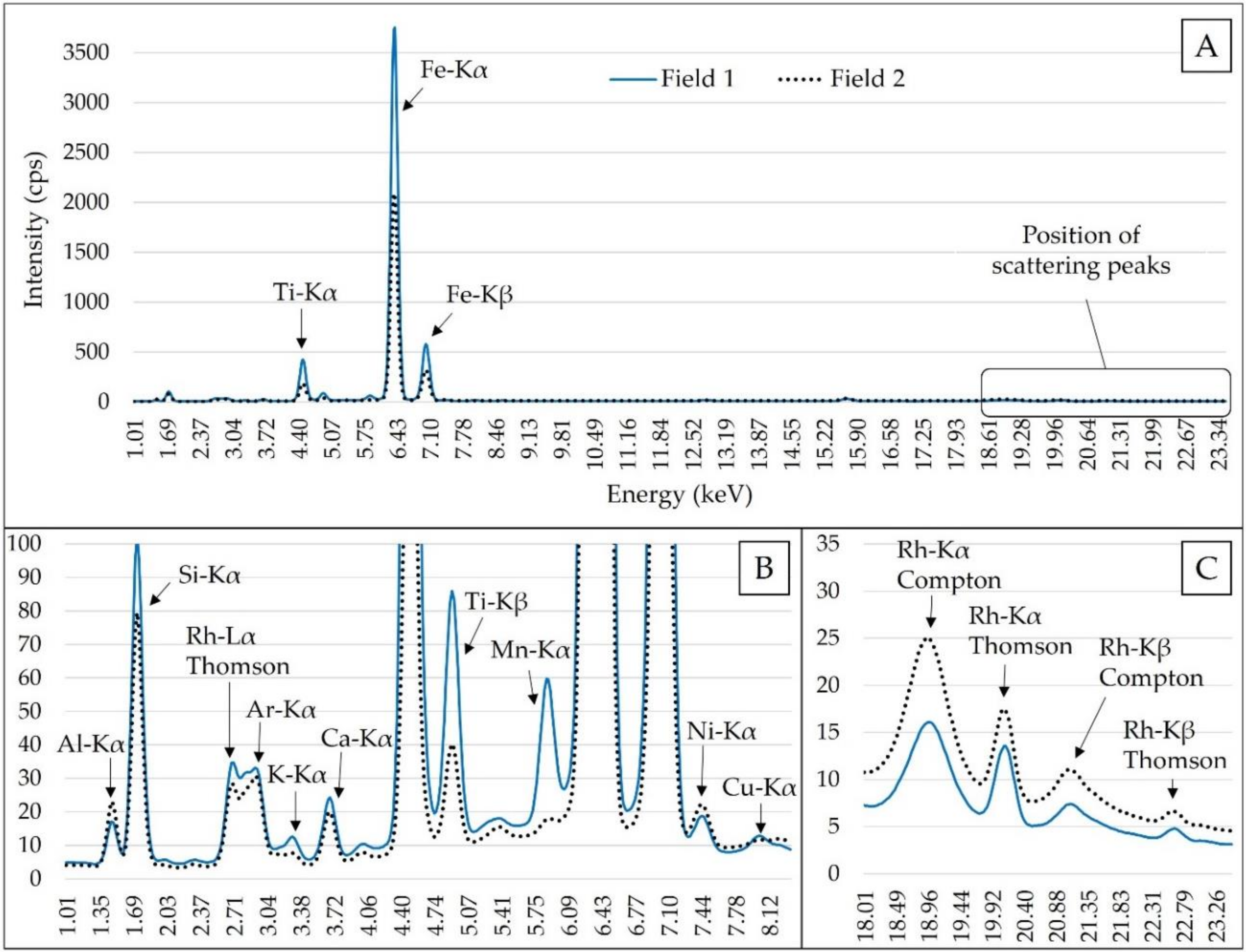
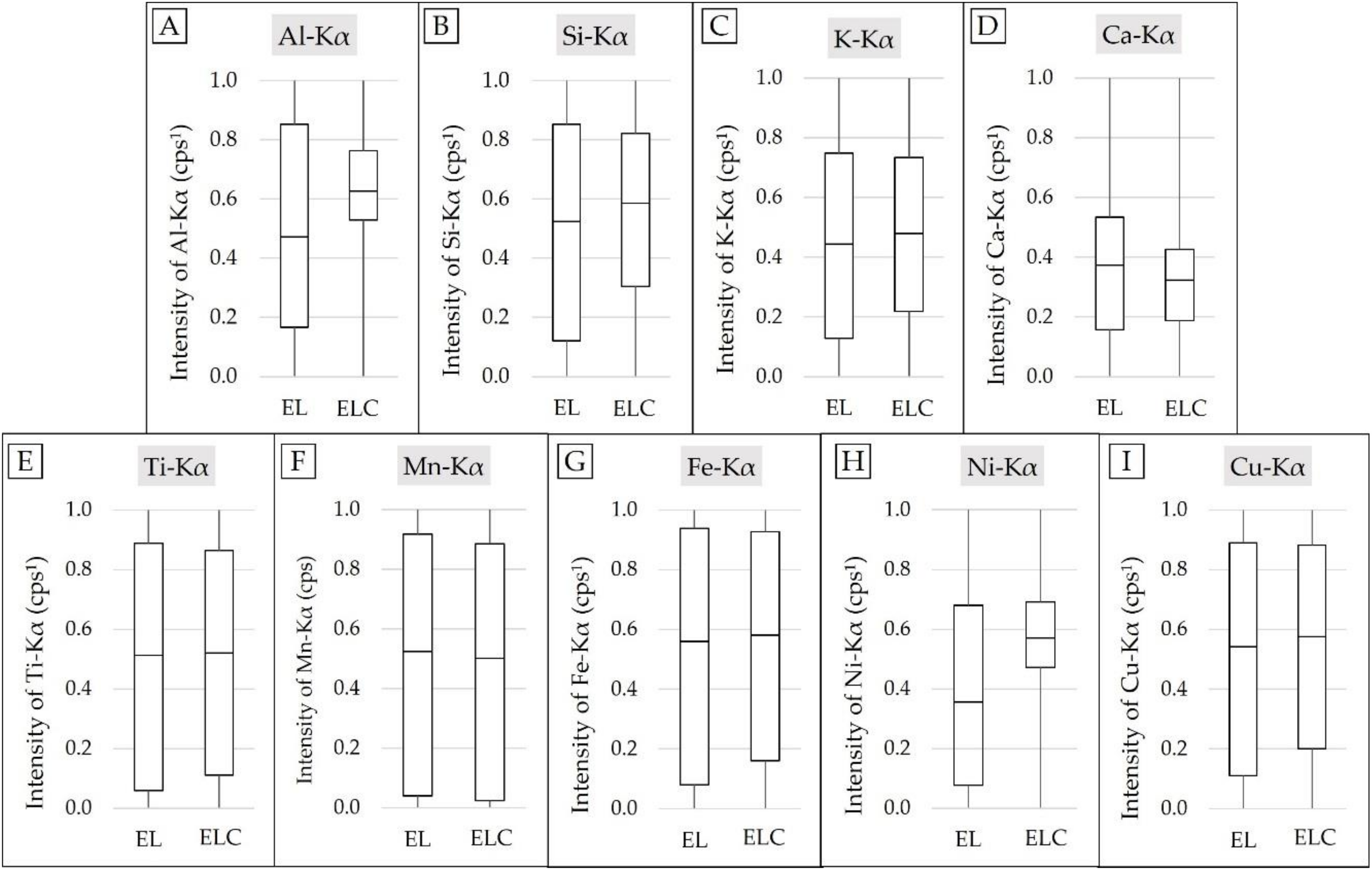
3.2. Effect of Compton Normalization on XRF Data

The ptc of the elements K, Ca, Ti, Mn, and Fe were compared with their respective emission lines in scatter plots made for two scenarios of with and without normalization by the Compton peak (Figure 4). Only K and Ca data showed continuous values when joining both fields (Figure 4A–D). The other elements (Ti, Mn, and Fe) presented a clear separation of data into contrasting groups, which highlights its different soil matrices. The scatter plots also show that the dispersion of XRF emission lines was reduced after being normalized by Compton peak, reducing its range between the first and third quartile (Figure 5). This is true for all evaluated emission lines except for Mn-Kα, whereas the largest rates of reductions are for the K-lines of Al, Ca, and Ni.
For both K and Ca of the two-field dataset, CN reduced dispersion, and improved the correlations between ptc and the K-lines of K and Ca, as R2 values increased from 0.84 to 0.89 for K, and from 0.69 to 0.92, for Ca (Figure 4A–D). The contrasting ranges leading to two clear groups of data for Ti, Mn, and Fe of the two fields resulted in an overestimation of R2. However, for these elements, it can be observed that CN did not lead to clear increases in the R2 values, as observed for Ca and K. The R2 values with and without CN were similar for Fe (R2 = 0.96, shown in Figure 4I,J), and slightly changed from 0.96 to 0.97 (Figure 4E,F) and from 0.98 to 0.97 (Figure 4G,H), for Ti and Mn, respectively.
Assessing the relationship between ptc and XRF emission lines for the Field 1 and Field 2 datasets separately, no clear performance improvement can be observed after the CN application on K-lines of K and Ca. Subtle performance reduction by CN for K and Ca is observed in Field 1, as R2 values were reduced from 0.46 to 0.43, for K, and from 0.83 to 0.81, for Ca. For Field 2, the R2 values for Ca-Kα slightly increased from 0.92 to 0.93. These results suggest a lower influence of CN on XRF data obtained from soil samples from the same field, confirming the lower influence of the matrix effect for individual field dataset, compared the dataset of the two fields.

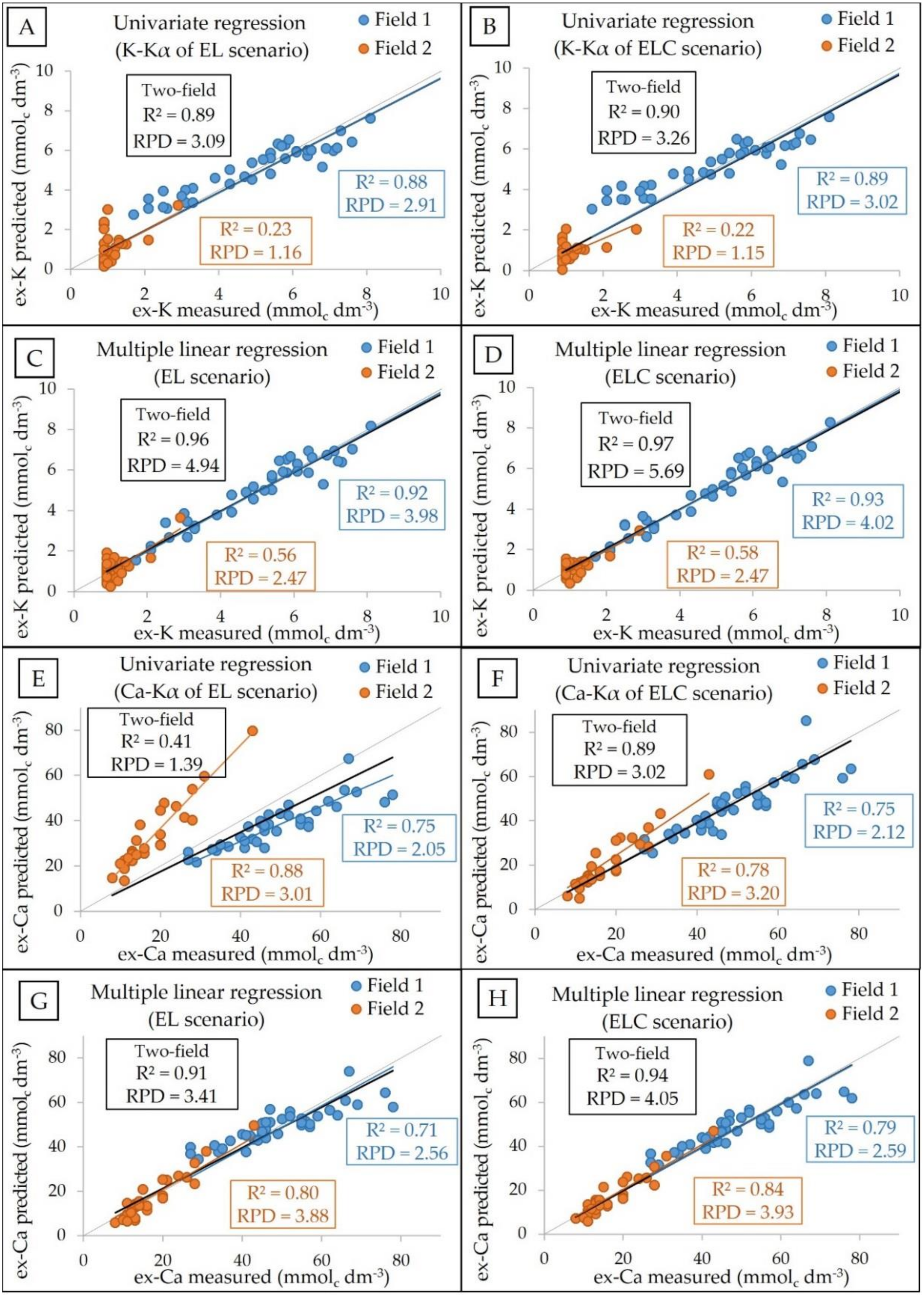
3.3. Matrix Effect Mitigation

3.3.1. Attenuation Promoted by Compton Normalization and MLR

The scatter plots of measured versus predicted ex-K and ex-Ca are presented in Figure 6A–H for calibrations with and without CN. For the two-field dataset, models for ex-Ca based on univariate regressions using the Ca-Kα without CN (Figure 6E) presented poor prediction performance (RPD = 1.39 and R2 = 0.41). This is clearly attributed to the different sample locations, confirming the matrix effect. An explicitly better prediction performance (RPD = 3.02 and R2 = 0.89) was obtained after CN, with points closely distributed around the 1:1 line, indicating the mitigation of part of the matrix effect present in the two-field dataset (Figure 6F). Even better prediction performance was observed for ex-Ca when using MLR (Figure 6G,H), with R2 and RPD values increasing from 0.91 and 3.41 for EL (Figure 6G) to 0.94 and 4.05 for ELC (Figure 6H). A similar trend with large matrix effect can be observed for CEC (Figure 6M–P), for which the prediction results of the univariate model improved from being of poor performance for EL (R2 = 0.35 and RPD = 1.25, Figure 6M) to reasonable performance with ELC (R2 of 0.64 and RPD of 1.95, Figure 6N). Again MLR for CEC prediction showed further improvement in the prediction performance of CEC (R2 ≥ 0.76 and RPD ≥ 2.07, Figure 6O,P), with the best performance obtained after the ELC scenario (R2 = 0.82 and RPD = 2.34, Figure 6P).
The ex-K prediction results (R2 and RPD values of 0.89 and 3.09, respectively) with univariate models using the K-Kα without CN did not indicate a distinguished matrix effect in the two-field dataset (Figure 6A), which may be related to the low dispersion of ex-K in Field 2, masking the visualization of matrix effect. However, the ex-K prediction after CN has slightly improved, with R2 and RPD values of 0.90 and 3.26, respectively (Figure 6B). Extra performance improvement was observed with MLR for ex-K prediction (Figure 6C,D).
Although the prediction results of clay using the univariate models were visually of good performances (0.80 ≤ R2 ≤ 0.85 and 2.28 ≤ RPD ≤ 2.60), point dispersions far from the 1:1 line indicating nonlinear behaviors, and consequently the clear matrix effect present in the two-field dataset (Figure 6I,J). Even CN did not lead to overcoming the matrix effect on clay prediction, behaving differently from the predictions for CEC, ex-K, and ex-Ca. With MLR, the clay prediction presented a linear dispersion of points around the 1:1 line with better performance indicators (R2 = 0.92 and RPD ≥ 3.64, Figure 6K,L). However, unlike observed for CEC, ex-K, and ex-Ca predictions, the MLR model after ELC did not show improvement in the prediction performance of clay, compared to the EL scenario. The observed R2 and RPD values for clay prediction using MLR were, respectively, 0.92 and 3.70, for the EL scenario (Figure 6K), and 0.92 and 3.64, for the ELC scenario (Figure 6L). Finally, the scatter plots of measured versus predicted ex-K, ex-Ca, clay, and CEC for calibrations using PLSR with and without CN are presented in Figure A1 (Appendix A). The PLSR models showed similar behavior to MLR, with all models showing a linear dispersion of points around the 1:1 line, as well as showing a slight increase in the prediction performance of ex-K, ex-Ca, and CEC for the ELC scenario in comparison with the EL scenario.
In summary, multivariate models (MLR and PLSR) for the prediction of ex-K, ex-Ca, clay, and CEC using both EL and ELC scenarios improved the linearity in the scatter plots, compared to the univariate models. In turn, CN has proved to be a good solution for mitigating the matrix effect in ex-K, ex-Ca, and CEC predictions, evidenced by increasing the predictive performance of these elements when used in both the univariate and multivariate models. However, CN was not useful for clay prediction, since no improvement in performance was observed in both the univariate and multivariate models.
It is also interesting to note that for predictions using individual field datasets the matrix effect was not as perceptible as seen for the two-field dataset. For the individual field models, the predictions with univariate regressions for EL showed a linear dispersion of points close the 1:1 line, particularly for ex-K in Field 1 (RPD = 2.91, Figure 6A), ex-Ca prediction in Field 1 (RPD = 2.05, Figure 6E), and clay in Field 2 (RPD = 1.43, Figure 6I).

3.3.2. Comparison Between MLR, PLSR, and the Geo Exploration Package

The results presented in Table 3 show comparable prediction performances for PLSR and MLR for both EL and ELC scenarios, with the biggest difference observed for clay prediction with the ELC scenario (R2 values of 0.92 and 0.89, for MLR and PLSR, respectively). Smaller differences than 0.03 of R2 values calculated for all properties indicate that both multivariate models tested allowed correcting the matrix effect present in the two-field dataset with comparable accuracies.
Again models developed after the CN (ELC scenario) provided subtly better prediction performances for all soil attributes evaluated. The only exception was the PLSR model for clay, which provided better results for the EL scenario (R2 of 0.91), compared to the ELC scenario (R2 of 0.89). The largest improvements after ELC were observed for CEC and ex-Ca models, either with MLR or PLSR, with an increase in R2 values for CEC of 0.04 and 0.06 and for ex-Ca of 0.04 and 0.05 for MLR and PLSR models, respectively. All other R2 increases, when using the ELC scenario, were less than 0.04.
Finally, results achieved using the Geo Exploration package data showed R2 values comparable to the MLR and PLSR models, with R2 values of 0.83 for CEC, 0.90 for ex-Ca, and 0.92 for clay and ex-K. Despite that, the prediction performances achieved using the Geo Exploration package data showed, in general, higher RMSE values. The only exception was the clay prediction, in which the Geo Exploration package presented the best result. For the other parameters (CEC, ex-K, and ex-Ca), the ELC models improved expressively the RMSE values. For CEC, the RMSE of PLSR-ELC model presented 21% lower than the one achieved by the Geo Exploration package; for ex-K, the MLR-ELC model presented a reduction of 26%; and for ex-Ca, the RMSE values of both PLSR-ELC and MLR-ELC reduced by 33% compared to the Geo Exploration package.

4. Discussion

Analyses of soil samples with heterogeneous composition using XRF sensors are subject to the called matrix effects. The matrix effect comprises the physical and chemical properties of the sample that influence the XRF spectra. Chemical matrix effects originate from differences in the concentrations of the elements that compose the soil matrix (e.g., concentrations of Fe, Si, Al, etc.), which generate interferences from absorption and/or enhancement of the fluorescence produced by the sample [28]. The total contents of Ti, Mn, Fe, and Cu and their emission lines, are different between both fields, confirming the matrix difference between them (Figure 4). Prediction models of the univariate calibration using the emission lines as input without CN showed a clear nonlinear dispersion of points around the 1:1 scatter plot line, with the samples divided into two groups according to their field of origin, especially for clay (Figure 6I), CEC (Figure 6M), and ex-Ca (Figure 6E) models. For ex-K, the matrix effect was less evident than the others, most probably due to the small variation range of this element in Field 2, as above commented (Section 3.1.).
The univariate calibration of clay, ex-Ca, and ex-K, used, respectively, the emission lines of Fe-Kα, Ca-Kα, and K-Kα; the Ca-Kα was also used for the prediction of CEC. These lines can suffer from an absorption effect depending on the presence of elements that have an absorption edge with slightly lower energy than their fluorescent peaks [42]. At the same time, enhancement effects may also occur due to the presence of elements that emit XRF with slightly higher energy than the absorption edge energy of these elements [28]. For example, Fe tends to absorb the Cu K-line, since Fe Kedge (7.11 keV) is close in energy to the Cu-Kα (8.05 keV), enhancing the intensity of Fe-Kα (6.41 keV). At the same time, Fe-Kα can be absorbed by the Cr, which presents Kedge at 5.99 keV, with energy slightly below that of Fe-Kα. Regarding the K-lines of K and Ca, the same interferences may take place between K (K-Kα = 3.31 keV and Kedge = 3.61 keV), Ar (Ar-Kα = 2.96 keV and Kedge = 3.20 keV), and Ca (Ca-Kα = 3.69 keV and Kedge = 4.04 keV), as well as between Ca, K, and Ti (Ti-Kα = 4.51 keV and Kedge = 4.97 keV).
The emission lines observed in this work presented well-defined peaks (Figure 3), indicating a low interference due to peak overlaps. However, chemical matrix effects due to spectral interferences can occur in soil samples, especially when heavier elements (e.g., Ba, Pb, W, etc.) are present in the soil matrix [43]. The energy of the L-lines of heavier elements occurs mainly within 0-10 keV, the region where the K-lines of important elements for soil assessment (e.g., Ti, Cr, Fe, Co, and Ni) exist and lead to increase the intensity of the K-lines measured by the detector [44]. Possible interference with K-Kα (3.31 keV) is the emissions of Cd-Lβ (3.33 keV) and Ti-Kα (4.51 keV) due to fluorescence of Ba-Lα (4.47 keV).
Solutions for matrix effect mitigation should be used to optimize the performance of prediction models in datasets with contrasting soil matrices [45]. In this work, the use of CN combined with multivariate regressions was tested as a potential solution to improve the prediction accuracy of selected fertility attributes. Our results showed that CN allowed correcting part of the matrix effect present in the two-field dataset for CEC, ex-K, and ex-Ca predictions. This is evident by comparing the results of the univariate models using the K-lines with and without CN. Better linearity of points scattered around the 1:1 line and greater prediction accuracy obtained after CN with RPD value increases of 0.70 for CEC (Figure 6M,N), 0.17 for ex-K (Figure 6A,B), and 1.63 for ex-Ca (Figure 6E,F). This was not true only for clay prediction, which may be explained by the large difference in intensity observed for the Fe-Kα emission line of the Field 1 and Field 2 datasets (Figure 4I,J). The clay prediction using the two-field dataset required employing MLR, which resulted in reducing the matrix effect (Figure 6A–D) by using a multilayer of information available in XRF data and improving the prediction accuracy of this variable. The principal variables for clay prediction were the K-lines of Fe, Ti, and Si (Table A1, Appendix A).
It should be noted that MLR without CN was sufficient to mitigate the error caused by the matrix effect and provide satisfactory prediction performances (R2 ≥ 0.76 and RPD ≥ 2.07) for clay, CEC, ex-K, and ex-Ca (Figure 6). These MLR models without CN had even slightly higher prediction performances than the corresponding univariate models after CN, with R2 value increases of 0.12 for clay (Figure 6J,K) and CEC (Figure 6N,O), 0.06 for ex-K (Figure 6B,C), and 0.02 for ex-Ca (Figure 6F,G). This may be explained by the fact that the multiple regressions account for emission lines of different elements that compose the soil matrix (e.g., Si, Al, Fe, Ti, etc.), which contain more information about the target element to be predicted than the single emission line accounted for by the univariate regression analysis [12,46]. The MLR-ELC scenario provided the best performance for the prediction of CEC, ex-K, and ex-Ca in the two-field dataset, reaching R2 ≥ 0.82 and RPD ≥ 2.34. The MLR-ELC outperformed MLR-EL by increasing the R2 values by 0.06, for CEC (Figure 6O,P), 0.01, for ex-K (Figure 6C,D), and 0.03, for ex-Ca (Figure 6G,H), while the prediction of clay remained similar in both scenarios, achieving R2 of 0.92 (Figure 6K,L).
Multivariate models including MLR and PLSR are better solutions to exploit the hidden information present in the spectra [31], mitigating the matrix effect while improving the prediction accuracy of fertility attributes. Comparing the predictive performances of PLSR and MLR models, it was observed that both performed similarly (Table 3). Panchuk et al. [31], reviewing the application of chemometric methods to XRF data, explained that PLSR models can perform similarly to MLR models when there are no overlaps in the emission lines selected for the models, otherwise PLSR models generally perform better than MLR. The spectra obtained in this work presented well-resolved peaks, which explain the similar prediction performance of MLR and PLSR models. In addition, results obtained with MLR and PLSR models showed prediction performances comparable to the Geo Exploration package (Table 3). These results indicate that the prediction performance of the multivariate models proposed in this paper may achieve a similar quality to those obtained by preprogrammed measurement packages (Table 3), and both approaches allowed the mitigation of the soil matrix effect. It is important to emphasize that preprogrammed measurement packages generally use calibration methods capable of correcting the matrix effect, as long as it is well-calibrated with accurate sensitivity coefficients.
In view of our results, a simple method for matrix effect mitigation by combining CN and multivariate models allowed a dataset of largely contrasting soil matrices, to be compatible for general calibrations of fertility attributes using XRF sensors. In general, the different strategies evaluated in this work can be presented in the following descending order of goodness of performance: multiple regressions using the selected emission lines after CN (ELC scenario) ≥ multiple regressions using the selected emission lines without CN (EC scenario) > univariate regression using emission lines after CN > univariate regression using emission lines without CN. Therefore, for the prediction of soil fertility attributes in datasets with the presence of matrix effect, we suggest the combined use of CN with any of the tested multivariate models (MLR or PLSR).
Most of the works that assessed XRF for predicting soil fertility attributes have used preprogrammed measurement packages [13,14,16,17,18,19,23,24,25], which use not disclosed general algorithms to preprocess the XRF data and mitigate the matrix effect [26]. Studies use these packages with a robust number (n ≥ 120) of soil samples reported R2 for clay prediction ranging between 0.85 and 0.97 [19,21], from 0.86 to 0.92, for CEC [14,16], from 0.67 to 0.81, for ex-K [16,18], and from 0.71 to 0.89, for ex-Ca [16,18]. The prediction accuracy for clay, CEC, ex-K, and ex-Ca observed in this research was similar or higher (Table 3) than those reported by the above-mentioned studies. Although preprogrammed measurement packages allow for a user-friendly approach that contributes to the popularization and expansion of the XRF application, they are not fully transparent and do not allow flexibility regarding the XRF scanning time [22]. Furthermore, the preprogrammed measurement packages offer total content values to be used as input for calibration models, which demand an extra validation step to confirm that the total contents are accurately measured. In general, accuracy problems with these routines can occur, which demands a “correction factor” that can be determined based on the ratio of the certified concentration of standard reference material and the XRF measured concentration [35,47,48]. In this sense, using intensity values of XRF emission lines is totally enough for establishing the prediction models avoiding this issue, and also the nonflexible procedures related to commercial packages (e.g., pre-established X-ray tube settings and scanning time).
Although the matrix effect presented clearly in the two-field dataset has been successfully mitigated in this work by combining CN and multivariate regressions, more investigations are needed to confirm that this approach can be applied for different datasets having different degrees of diversity of soil matrices. Therefore, it is essential that future research also evaluate other types of soils with contrasting soil characteristics that can proportionate distinct levels of chemical matrix effects, as well as evaluate more sophisticated methods for modeling XRF data (e.g., machine learning, and computational models), especially for calibrations involving a larger number of samples.

5. Conclusions

A portable X-ray fluorescence (XRF) sensor was used for the prediction of key soil fertility attributes (clay, cation exchange capacity (CEC), and exchangeable (ex-) K and Ca) in soil samples collected from two fields with contrasting soil matrices. In order to mitigate the matrix effect, solutions using Compton normalization (CN) combined with multivariate regressions (e.g., multiple linear regression (MLR) and partial least squares regression (PLSR)) were evaluated and compared to a modeling approach using both univariate and multivariate regression analyses without CN. In addition, the proposed solutions were also compared to modeling based on a preprogrammed measurement package approach (Geo Exploration package, Bruker AXS, Madison, WI, EUA).
Results showed that models developed with emission lines without CN were clearly affected by the matrix effect. For CEC, ex-K, and ex-Ca predictions, the matrix effect was attenuated by both CN and multivariate regressions (PLSR or MLR). For clay prediction the matrix effect was mitigated by the multivariate regressions only, for which CN had no effect. The prediction performances of MLR and PLSR models were comparable for all evaluated attributes. For the two-field dataset, the combined use of CN + multivariate regression achieved the best performances for the prediction of CEC (R2 = 0.82), ex-K (R2 = 0.97), and ex-Ca (R2 = 0.94), whereas comparable performance was recorded for clay with and without CN (R2 = 0.92). Therefore, it was suggested to use multivariate regressions (MLR or PLSR) combined with CN to predict key fertility attributes in sample sets with contrasting soil matrices.
The prediction performance observed for the solutions proposed in this work showed comparable results to the approach based on the Geo Exploration package, as well as to previously published works that used preprogrammed measurement packages. Moreover, the methodology applied in this study is simple and transparent, which allows the optimization of the procedures of XRF data acquisition, preprocessing, and modeling. Such knowledge is essential to enable more accurate and faster XRF analysis, as well as developing new applications of XRF sensors in the context of precision agriculture and soil science.

Author Contributions

Conceptualization, T.R.T. and J.P.M.; methodology, T.R.T., E.E.N.A., F.R.d.S., A.M.M., and F.L.M.; validation, E.E.N.A. and J.P.M.; formal analysis, T.R.T., E.E.N.A., A.M.M., and F.L.M.; investigation, T.R.T.; resources, T.R.T.; data curation, T.R.T.; writing—Original draft preparation, T.R.T., and A.M.M.; writing—Review and editing, E.E.N.A., F.L.M., F.R.d.S., H.W.P.d.C., A.M.M., and J.P.M.; visualization, T.R.T.; supervision, H.W.P.d.C., A.M.M., and J.P.M.; project administration, T.R.T., and J.P.M.; funding acquisition, T.R.T., J.P.M., and H.W.P.d.C. All authors have read and agreed to the published version of the manuscript.

Funding

The T.R.T. and E.E.N.A were funded by São Paulo Research Foundation (FAPESP), grant number 2017/21969-0 and 2018/08877-2, respectively; and also partially funded by the Brazilian Federal Agencies: Coordination for the Improvement of Higher Education Personnel (CAPES)—Finance Code 001, and the National Council for Scientific and Technological Development. (CNPq). XRF facilities were funded by FAPESP, grant 2015-19121-8, “Financiadora de Estudos e Projetos” (FINEP) project “Core Facility de suportes às pesquisas em Nutrologia e Segurança Alimentar na USP”, grant 01.12.0535.0, and INCT-FNA (Instituto Nacional de Ciência e Tecnologia - Física Nuclear e Aplicações), grant 464898/2014-5. Authors also acknowledge the financial support received from the Research Foundation—Flanders (FWO) for Odysseus I SiTeMan Project (Nr. G0F9216N).

Acknowledgments

We would like to thank the technician Eduardo de Almeida, from Laboratory of Nuclear Instrumentation, for the support with X-ray fluorescence equipment; and, also the technician Marina Colzato, from the Laboratory of Environmental Analysis, for the support with soil analysis.

Conflicts of Interest

The authors declare no conflicts of interest. The funders had no role in the design of the study; in the collection, analyses, or interpretation of data; in the writing of the manuscript, or in the decision to publish the results.

Appendix A

Table A1. Importance of X-ray fluorescence (XRF) variables for the prediction of studied soil fertility attributes on the two-field dataset, using both tested XRF scenarios, with (ELC scenario) and without (EL scenario) applying the Compton normalization to the selected emission lines. The values presented correspond to the t-value for each standardized coefficient obtained in the regressions calibration.
Al-KαSi-KαK-KαCa-KαTi-KαMn-KαFe-KαNi-KαCu-KαRh-Lα 3Rh-Kα 3Rh-Kα 4
ClayEL−1.1−2.4−1.3−0.4−2.8−0.55.2−1.1−1.2−1.20.1−0.8
ELC−0.6−4.3−1.1−0.4−2.5−0.13.1−1.2−1.7−1.71.1−2.5
CEC 1EL−0.5−0.41.54.62.5−1.6−0.41.30.8−0.80.0−0.2
ELC−0.3−0.51.45.93.3−1.20.80.90.9−0.2−0.71.8
ex-K 2EL−1.0−1.019.0−5.8−0.8−2.1−1.4−0.5−0.6−4.4−1.2−2.5
ELC−0.8−0.622.0−5.4−0.1−2.3−0.80.8−0.5−4.0−0.9−1.9
ex-Ca 2EL−1.10.81.09.2−0.2−1.80.51.10.60.81.5−1.3
ELC−1.30.61.011.9−0.4−1.00.90.70.51.31.50.1
1 Cation exchange capacity; 2 exchangeable (ex-) nutrients (ex-K and ex-Ca); 3 Thomson scattering peaks (Rh-Lα and Rh-Kα); 4 Compton scattering peak (Rh-Kα). The emboldened values indicate a significant correlation at the probability level of 0.05; significant values were presented on grayscale, with the most important variables having the darkest color and vice versa.
Figure A1. Scatter plots of measured versus predicted exchangeable (ex-) potassium (K; A,B), and calcium (Ca; C,D), clay (E,F), and cation exchange capacity (CEC; G,H) obtained with partial least squares regression (PLSR) using all selected emission lines from the EL (B,D,F,H) and ELC scenario (A,C,E,G). Models were obtained using the calibration set (n of 39, 29, and 68 for the Field 1, Field 2, and two-field dataset) and the validation was performed by “leave-one-out” full cross-validation. Figures of merit in blue, orange, and black correspond, respectively, to the calibrations performed using the Field 1, Field 2, and two-field datasets.
Agronomy 10 00787 g0a1

References

  1. Gebbers, R.; Adamchuk, V.I. Precision agriculture and food security. Science 2010, 327, 828–831. [Google Scholar] [CrossRef] [PubMed]
  2. Schirrmann, M.; Domsch, H. Sampling procedure simulating on-the-go sensing for soil nutrients. J. Soil Sci. Plant Nutr. 2011, 174, 333–343. [Google Scholar] [CrossRef]
  3. Molin, J.P.; Tavares, T.R. Sensor systems for mapping soil fertility attributes: Challenges, advances and perspectives in Brazilian tropical soils. Eng. Agric. 2019, 39, 126–147. [Google Scholar] [CrossRef] [Green Version]
  4. Rossel, R.A.V.; Adamchuk, V.I.; Sudduth, K.A.; Kenzie, N.J.M.; Lobsey, C. Proximal soil sensing: An effective approach for soil measurements in space and time. Adv. Agron. 2011, 113, 237–282. [Google Scholar] [CrossRef]
  5. Kuang, B.; Mahmood, H.S.; Quraishi, M.Z.; Hoogmoed, W.B.; Mouazen, A.M.; van Henten, E.J. Sensing soil properties in the laboratory, in situ, and on-line: A review. Adv. Agron. 2012, 114, 155–223. [Google Scholar] [CrossRef]
  6. Rossel, R.A.V.; Bouma, J. Soil sensing: A new paradigm for agriculture. Agric. Syst. 2016, 148, 71–74. [Google Scholar] [CrossRef]
  7. Mouazen, A.M.; Kuang, B. On-line visible and near infrared spectroscopy for in-field phosphorous Management. Soil Tillage Res. 2016, 155, 471–477. [Google Scholar] [CrossRef]
  8. Nawar, S.; Delbecque, N.; Declercq, Y.; Smedt, P.; Finke, P.; Verdoodt, A.; Meirvenne, M.V.; Mouazen, A.M. Can spectral analyses improve measurement of key soil fertility parameters with X-ray fluorescence spectrometry? Geoderma 2019, 350, 29–39. [Google Scholar] [CrossRef]
  9. Santos, F.R.; Oliveira, J.F.; Bona, E.; Santos, J.V.F.; Barboza, G.M.; Melquiades, F.L. EDXRF spectral data combined with PLSR to determine some soil fertility indicators. Microchem. J. 2020, 152, 104275. [Google Scholar] [CrossRef]
  10. Tavares, T.R.; Nunes, L.C.; Alves, E.E.N.; Almeida, E.; Maldaner, L.F.; Krug, F.J.; Carvalho, H.W.P.; Molin, J.P. Simplifying sample preparation for soil fertility analysis by X-ray fluorescence spectrometry. Sensors 2019, 19, 5066. [Google Scholar] [CrossRef] [Green Version]
  11. Gałuszka, A.; Migaszewski, Z.M.; Namieśnik, J. Moving your laboratories to the field—Advantages and limitations of the use of field portable instruments in environmental sample analysis. Environ. Res. 2015, 140, 593–603. [Google Scholar] [CrossRef] [PubMed]
  12. Morona, F.; Santos, F.R.; Brinatti, A.M.; Melquiades, F.L. Quick analysis of organic matter in soil by energy-dispersive X-ray fluorescence and multivariate analysis. Appl. Radiat. Isot. 2017, 130, 13–20. [Google Scholar] [CrossRef] [PubMed]
  13. Sharma, A.; Weindorf, D.C.; Man, T.; Aldabaa, A.A.A.; Chakraborty, S. Characterizing soils via portable X-ray fluorescence spectrometer: 3, Soil reaction (pH). Geoderma 2014, 232, 141–147. [Google Scholar] [CrossRef]
  14. Sharma, A.; Weindorf, D.C.; Wang, D.; Chakraborty, S. Characterizing soils via portable X-ray fluorescence spectrometer: 4, Cation exchange capacity (CEC). Geoderma 2015, 239, 130–134. [Google Scholar] [CrossRef]
  15. Rawal, A.; Chakraborty, S.; Li, B.; Lewis, K.; Godoy, M.; Paulette, L.; Weindorf, D.C. Determination of base saturation percentage in agricultural soils via portable X-ray fluorescence spectrometer. Geoderma 2019, 338, 375–382. [Google Scholar] [CrossRef]
  16. Silva, S.H.G.; Teixeira, A.F.D.S.; Menezes, M.D.D.; Guilherme, L.R.G.; Moreira, F.M.D.S.; Curi, N. Multiple linear regression and random forest to predict and map soil properties using data from portable X-ray fluorescence spectrometer (pXRF). Ciênc. Agrotecnol. 2017, 41, 648–664. [Google Scholar] [CrossRef]
  17. Teixeira, A.F.D.S.; Weindorf, D.C.; Silva, S.H.G.; Guilherme, L.R.G.; Curi, N. Portable X-ray fluorescence (pXRF) spectrometry applied to the prediction of chemical attributes in Inceptisols under different land uses. Ciênc. Agrotecnol. 2018, 42, 501–512. [Google Scholar] [CrossRef]
  18. Andrade, R.; Faria, W.M.; Silva, S.H.G.; Chakraborty, S.; Weindorf, D.C.; Mesquita, L.F.; Guilherme, L.R.G.; Curi, N. Prediction of soil fertility via portable X-ray fluorescence (pXRF) spectrometry and soil texture in the Brazilian Coastal Plains. Geoderma 2020, 357, 113960. [Google Scholar] [CrossRef]
  19. Zhu, Y.; Weindorf, D.C.; Zhang, W. Characterizing soils using a portable X-ray fluorescence spectrometer: 1. Soil texture. Geoderma 2011, 167, 167–177. [Google Scholar] [CrossRef]
  20. Silva, S.; Poggere, G.; Menezes, M.; Carvalho, G.; Guilherme, L.; Curi, N. Proximal sensing and digital terrain models applied to digital soil mapping and modeling of Brazilian Latosols (Oxisols). Remote Sens. 2016, 8, 614. [Google Scholar] [CrossRef] [Green Version]
  21. Lima, T.M.; Weindorf, D.C.; Curi, N.; Guilherme, L.R.; Lana, R.M.; Ribeiro, B.T. Elemental analysis of Cerrado agricultural soils via portable X-ray fluorescence spectrometry: Inferences for soil fertility assessment. Geoderma 2019, 353, 264–272. [Google Scholar] [CrossRef]
  22. Tavares, T.R.; Molin, J.P.; Nunes, L.C.; Alves, E.E.N.; Melquiades, F.L.; Carvalho, H.W.P.; Mouazen, A.M. Effect of X-ray tube configuration on measurement of key soil fertility attributes with XRF. Remote Sens. 2020, 12, 963. [Google Scholar] [CrossRef] [Green Version]
  23. Weindorf, D.C.; Zhu, Y.; Daniel, P.M.; Valerio, M.; Lynn, L.; Michaelson, G.; Clark, M.; Ping, C.L. Characterizing soils via portable X-ray fluorescence spectrometer: 2. Spodic and Albic horizons. Geoderma 2012, 189, 268–277. [Google Scholar] [CrossRef]
  24. O’Rourke, S.M.; Stockmann, U.; Holden, N.M.; Bratney, A.B.M.; Minasny, B. An assessment of model averaging to improve predictive power of portable vis-NIR and XRF for the determination of agronomic soil properties. Geoderma 2016, 279, 31–44. [Google Scholar] [CrossRef]
  25. Silva, E.A.; Weindorf, D.C.; Silva, S.H.; Ribeiro, B.T.; Poggere, G.C.; Carvalho, T.S.; Goncalves, M.G.; Guilherme, L.R.; Curi, N. Advances in Tropical Soil Characterization via Portable X-Ray Fluorescence Spectrometry. Pedosphere 2019, 29, 468–482. [Google Scholar] [CrossRef]
  26. Bowers, C. Matrix Effect Corrections in X-ray Fluorescence Spectrometry. J. Chem. Educ. 2019, 96, 2597–2599. [Google Scholar] [CrossRef]
  27. Weindorf, D.C.; Chakraborty, S. Portable X-ray fluorescence spectrometry analysis of soils. In Methods of Soil Analysis; Hirmas, D., Madison, W.I., Eds.; Soil Science Society of America: Wisconsin, WI, USA, 2016; pp. 1–8. [Google Scholar] [CrossRef]
  28. USEPA—United States Environmental Protection Agency (2007) Method 6200: Field portable X-ray Fluorescence Spectrometry for the Determination of Elemental Concentrations in Soil and Sediment. Available online: https://www.epa.gov/sites/production/files/2015-12/documents/6200.pdf (accessed on 25 March 2020).
  29. Kalnicky, D.J.; Singhvi, R. Field portable XRF analysis of environmental samples. J. Hazard. Mater. 2001, 83, 93–122. [Google Scholar] [CrossRef] [Green Version]
  30. Yılmaz, D.; Boydaş, E. The use of scattering peaks for matrix effect correction in WDXRF analysis. Radiat. Phys. Chem. 2018, 153, 17–20. [Google Scholar] [CrossRef]
  31. Panchuk, V.; Yaroshenko, I.; Legin, A.; Semenov, V.; Kirsanov, D. Application of chemometric methods to XRF-data—A tutorial review. Anal. Chim. Acta 2018, 1040, 19–32. [Google Scholar] [CrossRef]
  32. IUSS Working Group WRB. World reference base for soil resources 2014. In World Soil Resources Reports No. 106; Schad, P., van Huyssteen, C., Micheli, E., Eds.; FAO: Rome, Italy, 2014; p. 189. ISBN 978-92-5-108369-7. [Google Scholar]
  33. Van Raij, B.; Andrade, J.C.; Cantarela, H.; Quaggio, J.A. Análise Química Para Avaliação de Solos Tropicais; IAC: Campinas, Brazil, 2001; p. 285. (In Portuguese) [Google Scholar]
  34. Element, C.A.S. Method 3051A microwave assisted acid digestion of sediments, sludges, soils, and oils. Z. Für Anal. Chem. 2007, 111, 362–366. [Google Scholar]
  35. Mantler, M.; Willis, J.P.; Lachance, G.R.; Vrebos, B.A.R.; Mauser, K.E.; Kawahara, N.; Rousseau, R.M.; Brouwer, P.N. Quantitative analysis. In Handbook of Practical X-Ray Fluorescence Analysis; Burkhard, B., Kanngiesser, B., Langhoff, N., Wedell, R., Wolff, H., Eds.; Springer: Berlin/Heidelberg, Germany, 2006; pp. 309–410. [Google Scholar]
  36. Currie, L.A. Limits for qualitative detection and quantitative determination. Application to radiochemistry. Anal. Chem. 1968, 40, 586–593. [Google Scholar] [CrossRef]
  37. Nogueirol, R.C.; De Melo, W.J.; Bertoncini, E.I.; Alleoni, L.R.F. Concentrations of Cu, Fe, Mn, and Zn in tropical soils amended with sewage sludge and composted sewage sludge. Environ. Monit. Assess. 2013, 185, 2929–2938. [Google Scholar] [CrossRef]
  38. Silva, Y.J.A.B.; Nascimento, C.W.A.; Biondi, C.M. Comparison of USEPA digestion methods to heavy metals in soil samples. Environ. Monit. Assess. 2014, 186, 47–53. [Google Scholar] [CrossRef]
  39. Kennard, R.W.; Stone, L.A. Computer aided design of experiments. Technometrics 1969, 11, 137–148. [Google Scholar] [CrossRef]
  40. Chang, C.W.; Laird, D.A.; Mausbach, M.J.; Hurburgh, C.R. Near-infrared reflectance spectroscopy-principal components regression analyses of soil properties. Soil Sci. Soc. Am. J. 2001, 65, 480–490. [Google Scholar] [CrossRef] [Green Version]
  41. Van Raij, B. Fertilidade Do Solo e Manejo de Nutrientes; International Plant Nutrition Institute (IPNI): Piracicaba, São Paulo, Brazil, 2011; p. 420. (In Portuguese) [Google Scholar]
  42. Jenkins, R. X-Ray Fluorescence Spectrometry; John Wiley & Sons: Hoboken, NJ, USA, 2012; p. 232. [Google Scholar]
  43. Taggart, J.E., Jr.; Lindsay, J.R.; Scott, B.A.; Vivit, D.V.; Bartel, A.J.; Stewart, K.C. Analysis of geologic materials by wavelength-dispersive X-ray fluorescence spectrometry. In Methods for Geochemical Analysis; US Geological Survey Bulletin: Denver, CO, USA, 1987; Volume 1770, pp. 1–19. [Google Scholar]
  44. Gallhofer, D.; Lottermoser, B.G. The influence of spectral interferences on critical element determination with portable X-ray fluorescence (pXRF). Minerals 2018, 8, 320. [Google Scholar] [CrossRef] [Green Version]
  45. Markowicz, A.A. Chapter 2 quantification and correction procedures. In Portable X-ray Fluorescence Spectrometry: Capabilities for In Situ Analysis; The Royal Society of Chemistry: London, UK, 2008; pp. 13–38. [Google Scholar]
  46. Kaniu, M.I.; Angeyo, K.H.; Mangala, M.J.; Mwala, A.K.; Bartilol, S.K. Feasibility for chemometric energy dispersive X-ray fluorescence and scattering (EDXRFS) spectroscopy method for rapid soil quality assessment. X-Ray Spectrom. 2011, 40, 432–440. [Google Scholar] [CrossRef]
  47. Koch, J.; Chakraborty, S.; Li, B.; Kucera, J.M.; Van Deventer, P.; Daniell, A.; Faul, C.; Man, T.; Pearson, D.; Duda, B.; et al. Proximal sensor analysis of mine tailings in South Africa: An exploratory study. J. Geochem. Explor. 2017, 181, 45–57. [Google Scholar] [CrossRef]
  48. Chakraborty, S.; Li, B.; Weindorf, D.C.; Deb, S.; Acree, A.; De, P.; Panda, P. Use of portable X-ray fluorescence spectrometry for classifying soils from different land use land cover systems in India. Geoderma 2019, 338, 5–13. [Google Scholar] [CrossRef]
Figure 1. Framework of the methodology applied for the development of calibration models for clay, cation exchange capacity (CEC), and exchangeable (ex-) potassium (K) calcium (Ca), and magnesium (Mg), using portable X-ray fluorescence device (pXRF) and methods to attenuate the matrix effect. Two scenarios of XRF data preprocessing (emission lines with (ELC) and without (EL) Compton normalization), both using the 12 emission lines selected (Al-Kα, Si-Kα, K-Kα, Ca-Kα, Ti-Kα, Mn-Kα, Fe-Kα, Ni-Kα, Cu-Kα, Rh-Lα Thomson, Rh-Kα Thomson, and Rh-Kα Compton), were subjected to multiple linear regression (MLR) and partial least squares regression (PLSR) analyses. For the ELC scenario, the fluorescence emission lines of Al-Kα, Si-Kα, K-Kα, Ca-Kα, Ti-Kα, Mn-Kα, Fe-Kα, Ni-Kα, and Cu-Kα were normalized by the Compton peak, which was not applied for the EL scenario. Scattering peaks were not normalized in any of the scenarios. Total contents obtained with the Geo Exploration package (Bruker AXS, Madison, WI, USA) were also used to calibrate models for the studied soil attributes using MLR, having their performance compared with the other calibrated models.
Agronomy 10 00787 g001
Figure 2. Location of Field 1 and Field 2 in Brazil, where the soil samples were collected.
Agronomy 10 00787 g002
Figure 3. Mean of X-ray fluorescence (XRF) spectra of Field 1 and Field 2 (A). Snapshot of the emission lines from 1.01 to 8.34 keV, focusing on the elements that presented lower XRF emission intensity in relation to the Kα emission lines of iron (Fe) (B). Snapshot of the scattering region of Rh K-lines (C). Counts of photons per second were abbreviated as cps.
Agronomy 10 00787 g003
Figure 4. Scatter plots of measured pseudo total content (ptc) of potassium (K), calcium (Ca), titanium (Ti), manganese (Mn), and iron (Fe) versus their respective K-line intensity. The scatter plots were presented for the emission lines of both EL (on the left side, A,C,E,G,I) and ELC scenarios (on the right side, B,D,F,H,J). The intensity of the emission lines was presented in counts per second (cps), and the cps were normalized by Compton peak (cps*). The coefficient of determination (R2) of each scatter plot was also presented. The points and R2 presented in blue, orange, and black correspond, respectively, to the data of the Field 1, Field 2, and two-field datasets.
Agronomy 10 00787 g004
Figure 5. Box plots of the K-lines intensity of aluminum (Al), silicon (Si), potassium (K), calcium (Ca), titanium (Ti), manganese (Mn), iron (Fe), nickel (Ni), and copper (Cu; AI, respectively) from the EL and ELC scenarios. The counts per second were scaled (cps1) using their maximum and minimum values in order to represent the intensity of both scenarios on a comparable scale.
Agronomy 10 00787 g005
Figure 6. Scatter plots of measured versus predicted exchangeable (ex-) potassium (K; AD) and calcium (Ca; EH), clay (IL), and cation exchange capacity (CEC; MP) obtained from univariate regression using the K-lines without the Compton normalization (EL scenario; A,E,I,M, respectively); univariate regression using the K-lines after the Compton normalization (ELC scenario; B,F,J,N, respectively); multiple linear regression using all selected emission lines from the EL scenario (C,G,K, and O, respectively); and multiple linear regression using all selected emission lines from the ELC scenario (D,H,L,P, respectively). Models were obtained using the calibration set (n of 39, 29, and 68 for the Field 1, Field 2, and two-field datasets) and the validation was performed by “leave-one-out” full cross-validation. Figures of merit in blue, orange, and black correspond, respectively, to the calibrations performed using the Field 1, Field 2, and two-field datasets.
Agronomy 10 00787 g006aAgronomy 10 00787 g006b
Table 1. Descriptive statistics of the studied soil fertility attributes according to the calibration and validation set used for each dataset evaluated.
Clay 1CEC 1ex-K 1ex-Ca 1
Cal SetVal SetCal SetVal SetCal SetVal SetCal SetVal Set
Field 1 2
Min345.00378.0058.9062.501.702.3027.0028.00
Mean424.03405.4797.5293.235.115.0749.2147.53
Max511.00463.00148.90138.4010.307.9078.0075.00
SD44.1024.5220.9321.191.941.5012.5313.52
CV (%)10.406.0521.4622.7337.9229.4825.4728.44
Field 2 2
Min175.00175.0037.5042.500.900.908.008.00
Mean255.14239.2060.5455.311.121.1917.5215.33
Max328.00328.0088.9088.902.902.3043.0038.00
SD45.9051.3413.8913.130.430.397.817.78
CV (%)17.9921.4622.9423.7438.3833.2344.5850.74
Two-field 2
Min175.00175.0037.5042.500.900.908.008.00
Mean352.00332.1281.7576.503.413.3635.6933.32
Max511.00463.00148.90138.4010.307.9078.0075.00
SD95.2192.0325.8626.142.482.2619.0819.71
CV (%)27.0527.7131.6334.1772.7367.3953.4459.16
1 The minimum (min), maximum (max), mean, and standard deviation (SD) values of clay content were given in g dm−3 and, in mmolc dm−3, for cation exchange capacity (CEC) and the exchangeable (ex-) contents of K and Ca. 2 The number of samples (n) used for the calibration (cal) and validation (val) sets were, respectively, 39 and 19 for the Field 1 dataset, 29 and 15 for the Field 2 dataset, and 68 and 34 for the two-field dataset.
Table 2. Pearson’s correlation between the studied soil fertility attributes for each dataset evaluated. Correlations between exchangeable (ex-) and pseudo total content (ptc) of potassium (K) and calcium (Ca) are also shown.
ClayCEC 1ex-K 2ex-Ca 2ClayCECex-Kex-CaClayCECex-Kex-Ca
Field 1Field 2Two-field dataset
Clay1.00−0.02−0.050.141.000.31 *0.34 *0.211.000.67 **0.73 **0.78 **
CEC 1.000.170.93 ** 1.000.010.70 ** 1.000.64**0.93 **
ex-K 1.000.03 1.00−0.01 1.000.68 **
ex-Ca 1.00 1.00 1.00
Correl 3 with ptc 0.67 **0.83 ** 0.49 **0.95 ** 0.90 **0.75 **
* Significant correlation at the probability level of 0.05; ** Significant correlation at the probability level of 0.01; the correlations were presented on grayscale highlighting the highest values. 1 Cation exchange capacity. 2 Exchangeables (ex-) K and Ca 3 Pearson’s coefficient of correlation (r).
Table 3. Prediction results of the validation set (n = 34) obtained from multiple linear regressions (MLR) and partial least squares regression (PLSR) using portable X-ray fluorescence (XRF) measured emission lines with (ELC) and without (EL) Compton normalization. The results obtained with MLR using the Geo Exploration package data as input X-variables were also shown.
Geo Exp. Package 3MLRPLSR
ELELCELELCnLV 4
R 2
Clay0.920.910.920.910.894
CEC 10.830.830.870.810.873
ex-K 20.920.920.950.910.943
ex-Ca 20.900.920.960.910.964
RMSE
Clay27.4431.7229.4032.6535.564
CEC11.9011.0810.1911.569.423
ex-K0.720.650.530.750.603
ex-Ca6.095.634.095.994.114
RPD
Clay3.352.903.132.822.594
CEC2.202.362.572.262.783
ex-K3.163.474.263.013.773
ex-Ca3.243.504.823.294.804
1 Cation exchange capacity; 2 exchangeable (ex-) nutrients (ex-K and ex-Ca); 3 Geo Exploration package (Bruker AXS, Madison, WI, EUA); 4 number of latent variables used for the PLSR models calibrated for both EL and ELC scenarios. The coefficient of determination (R2) and residual prediction deviation (RPD) values are presented on grayscale, highlighting the highest values. The root-mean-square error (RMSE) was given in g dm−3 for clay, and in mmolc dm−3 for CEC, ex-K, and ex-Ca.

