Article

Cut-Edge Detection Method for Rice Harvesting Based on Machine Vision

Key Laboratory of Modern Precision Agriculture System Integration Research, Ministry of Education, China Agricultural University, Beijing 100083, China
*
Author to whom correspondence should be addressed.
Agronomy 2020, 10(4), 590; https://doi.org/10.3390/agronomy10040590
Submission received: 18 March 2020 / Revised: 15 April 2020 / Accepted: 17 April 2020 / Published: 20 April 2020
(This article belongs to the Special Issue Precision Agriculture for Sustainability)

Abstract

:
A cut-edge detection method based on machine vision was developed for obtaining the navigation path of a combine harvester. First, the Cr component in the YCbCr color model was selected as the grayscale feature factor. Then, by detecting the end of the crop row, judging the target demarcation and getting the feature points, the region of interest (ROI) was automatically gained. Subsequently, the vertical projection was applied to reduce the noise. All the points in the ROI were calculated, and a dividing point was found in each row. The hierarchical clustering method was used to extract the outliers. At last, the polynomial fitting method was used to acquire the straight or curved cut-edge. The results gained from the samples showed that the average error for locating the cut-edge was 2.84 cm. The method was capable of providing support for the automatic navigation of a combine harvester.

1. Introduction

The invention of the harvester has led to an improvement in the production efficiency. However, during harvest the driver needs to continuously adjust those parameters such as speed, direction as well as cutting width [1,2], which inevitably increases operator fatigue. The invention of the automatic navigation technology of the harvester can effectively reduce the driver′s work intensity while improving the operating efficiency, which is of great significance [3].
The extraction of the navigation path is crucial for automatic navigation. Traditionally, the cut/uncut edge is often used as the reference for the harvester’s working path. The driver needs to steer the harvester along this cut-edge. Therefore, the technology of automatically detecting the cut-edge is one of the key technologies of the automatic navigation system of the harvester.
At present, Global Navigation Satellite System (GNSS), Light Detection and Ranging (LiDAR), and vision sensors are often used as main detection devices in automatic navigation systems, while the millimeter-wave radar, ultrasonic radar and infrared cameras are mainly used as the auxiliary part [4,5,6]. Now, agricultural machinery navigation systems based on the Real-time kinematic (RTK) GNSS have been adopted and are widespread [7]. However, the RTK GNSS costs a considerable amount and it can only provide navigation according to a predetermined path and can’t solve the external sensing problem. Therefore, other sensors are also needed in the navigation system to achieve the real-time environment detection. Although LiDAR is known for a long detection range and high accuracy [8], it is also high cost and know for its sparse point cloud. LiDAR is greatly affected by dust and straw debris, which means that it is not suitable to use in harvesting environments. The vision sensor is characterized by a high resolution, large amount of information and a low cost [9]. The machine vision is used to detect lateral and heading deviations of the agricultural machinery from the expected working path. This method can be applied for unknown environments, irregular fields, or environments where GNSS signals cannot be received.
Based on the above analysis, to meet the needs of small-scale rice fields and non-linear operations, this study used visual sensors as sensing devices. However, the following issues needed to be addressed in a complex field environment:
  • the irregular cut-edge.
  • great variability in relatively smaller areas caused by rice texture.
  • dynamic changes in image brightness and color temperature.
  • blurry images and weakened texture features caused by the harvester vibrations.
  • the interference in the image.
To solve the above problems, this research, based on visual sensors, explored the cut-edge detection method in the work environment to make it more robust under field conditions.
Table 1 illustrates the research on the visual detection of the cut-edge, which could be classified into three groups: detection based on color, on texture and on stereo vision.
The stereo-vision-based method uses the height difference between the crops and the land to identify crop rows [22]. Although this method is not affected by shadows, it only works for tall crops and cannot effectively identify crop rows cut by a semi-feeder harvester.
The texture feature can be used to detect the cut-edge [23], but the vibrations of the harvester will blur the image and weaken the texture feature which would also be affected by light changes.
The color-based segmentation method uses the color difference between the cut and un-cut areas for segmentation, which is characterized by a small amount of calculation and high accuracy [24]. However, this method is greatly affected by light changes and shadows and is not suitable for crops with low color discrimination such as wheat.
Because the color difference between the cut and uncut areas is relatively stable during the rice harvesting, it was advisable to use color to segment the image. Current extraction methods have limitations such as the lack of robustness under a complex light and susceptibility to trees and roads. Therefore, improving the robustness of the color segmentation method and eliminating the interference factors were the focus of this study.

2. Materials and Methods

2.1. Image Collection

2.1.1. Image Collection System

The image collection system was installed on the combine harvester to capture and process the image in real time. The system was composed of vision sensors, mounting brackets, transmission cables and on-board computers.
The vision sensor was an Olympus EM1 Mark ii camera, which can provide five-axis body image stabilization to reduce the impact of the shaking caused by the combine harvester. The size of the image is 960 × 960 pixels and the collection frequency is 1Hz. The on-board computer was a Dell Precision 7530 mobile workstation.
Figure 1 illustrates the general layout of the system. The two cameras were installed directly above both sides of the header. The cameras were connected to the mounting bracket through a spherical head, which made it possible for them to adjust the shooting elevation angle. The camera near the cut-edge was turned on to cope with the combine harvester′s clockwise and counterclockwise operation. During the harvest, the camera was directly above the cut-edge. When controlling the steering angle of the vehicle, a driver only needed to keep the cut-edge in the center of the screen.

2.1.2. Prior Conditions for the Picture

The method proposed in this study worked only for the cases where the following prior conditions were met:
  • The picture contained one or more cut-edges and there was only one cut-edge at the bottom of the picture.
  • The target cut-edge started from the bottom of the screen and extended to the distance without a return.
  • The target cut-edge was a single-valued function of row coordinates.

2.2. Grayscale Feature Factor Section

To improve the contrast between the cut and uncut areas, which is to reduce the intra-regional differences while increasing the inter-regional differences, it was necessary to compare the grayscale feature factors, and select the color space and components suitable for the rice harvesting scene [25].
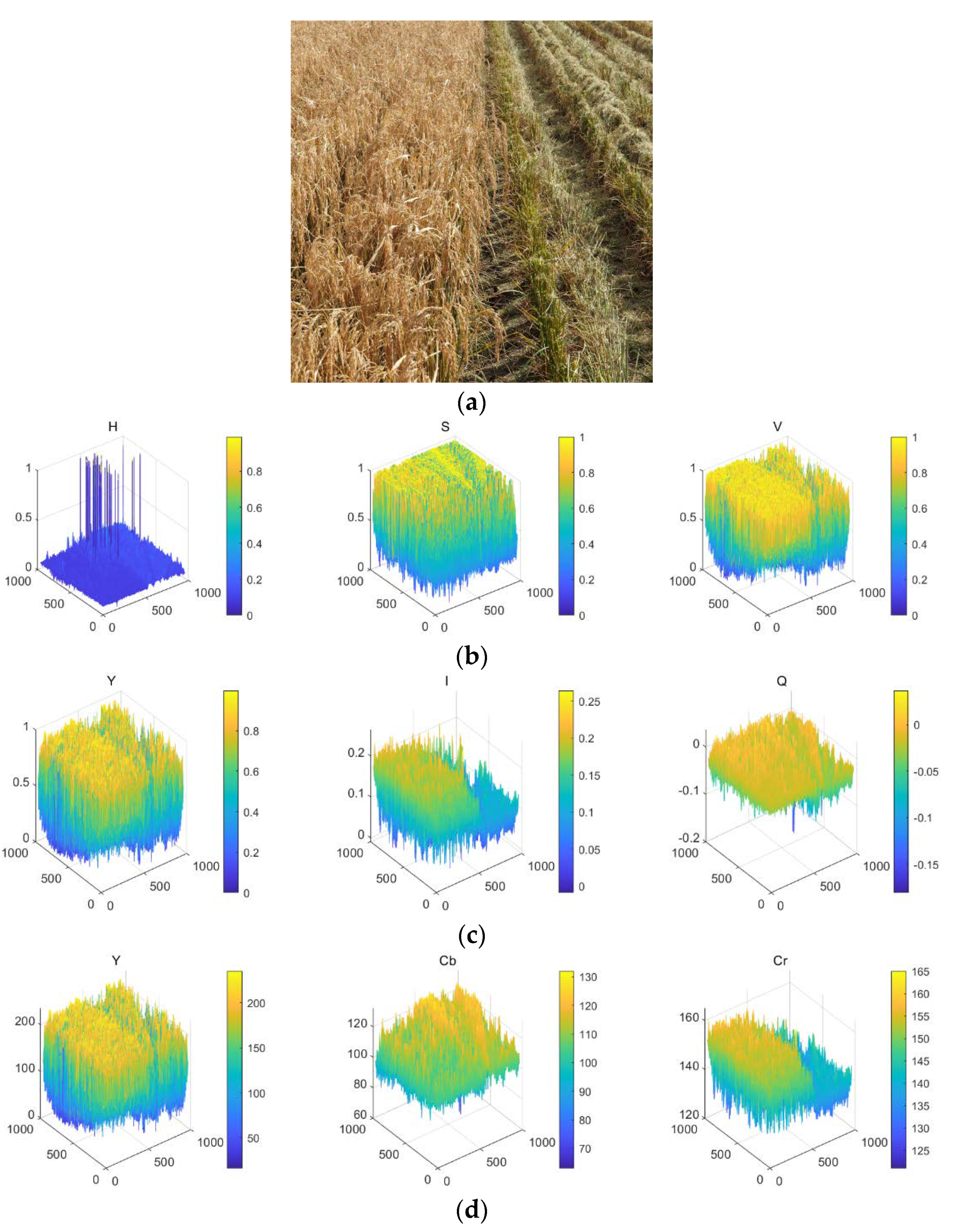
The RGB images collected by the camera were converted to color spaces containing separate brightness components such as the HSV, YCbCr and the NTSC so that the effects of the light changes and shadows could be reduced [26]. Take Figure 2a as an example to view the different components in each color space. The results are shown in Figure 2b–d.
According to the statistical results, under the rice harvesting conditions, the Cr component in the YCbCr color space was characterized by the feature that its intra-regional variability was relatively low while its inter-regional difference was relatively high. It was therefore used as a processing project. The following studies were based on images gray-scaled by the Cr component in the YCbCr model.

2.3. Region of Interest (ROI) Extraction

To reduce the scanning range and the computation, and eliminate interference factors such as trees and roads, it was necessary to automatically obtain the region of interest (ROI). The ROI included the following characteristics:
  • There was only one cut-edge starting from the bottom and extending to the top.
  • There were only cut and uncut areas that existed.
  • The region containing the target cut-edge was as small as possible.
The steps of creating the ROI included an end-of-row detection, target crop row selection and ROI extraction.

2.3.1. End-of-Row Detection

The end-of-row needed to be detected since there was a non-interest area, as well as many interference factors outside the end of the row.
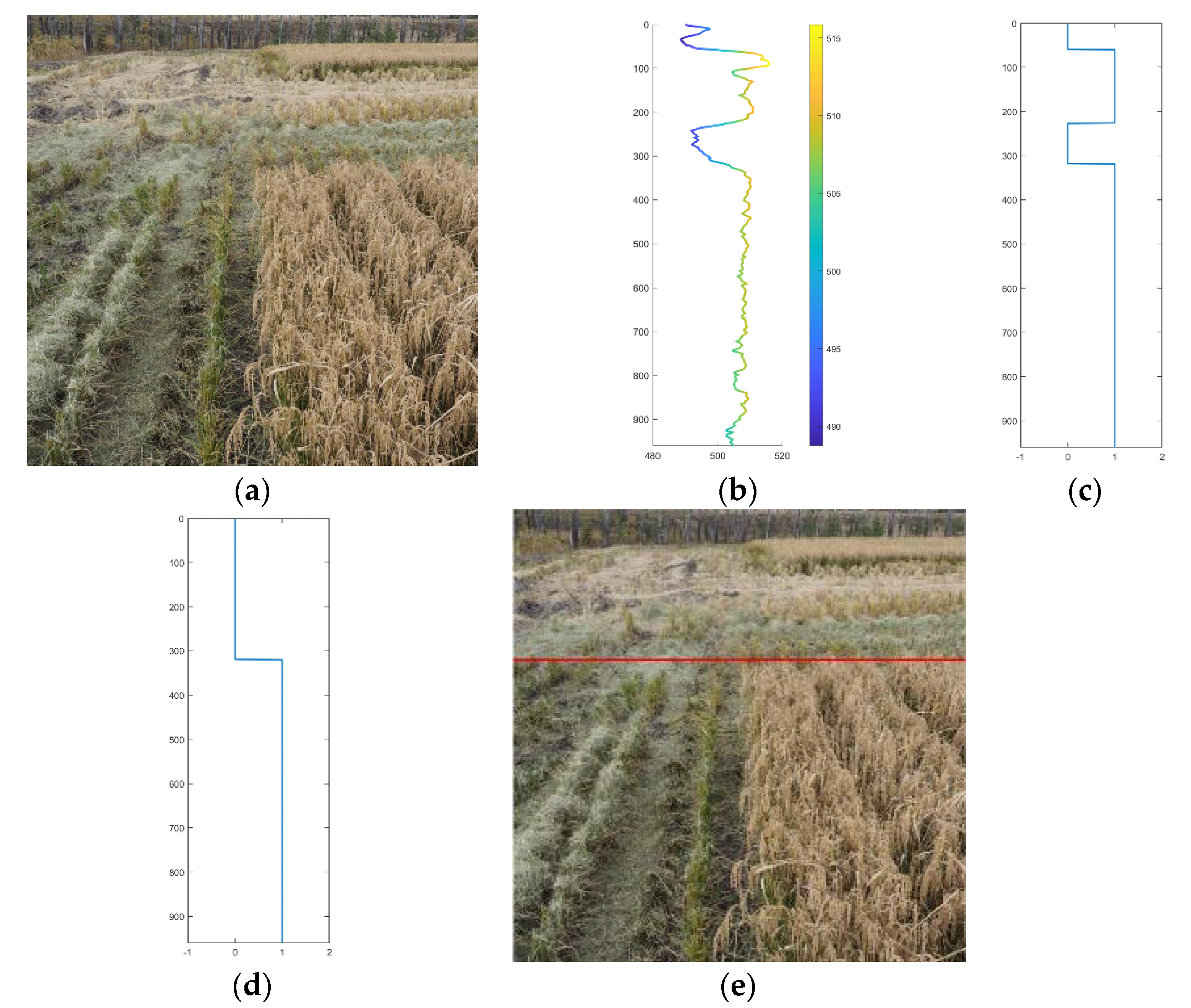
The image was horizontally projected (Figure 3a) and accumulated pixels of each row according to formula (1):
P i = 1 j n P ( i , j )
In formula (1), P(i, j) represents the pixel value of the i-th row and j-th column, and n is the number of the column of the image.
The projection result is shown in Figure 3b. The image shows good consistency in ROI. There was a clear valley boundary between ROI and non-ROI.
The projection result was shaped according to formula (2). The threshold was set to the average of the maximum and minimum values:
P i { = 1 , P i   ( max ( P ) min   ( P ) ) / 2 = 0 , P i < ( max ( P ) min   ( P ) ) / 2
In formula (2), Pi is the projection result of the i-th row, max (P) and min (P) are the maximum and minimum values in the projection result.
The effect after shaping is shown in Figure 3c. The area below the waveform is the vertical range of the ROI. Only the value of the ROI was retained. The result is shown in Figure 3d. The image is divided at the end-of-row and the detection result is shown in Figure 3e.

2.3.2. Target Crop Row Selection

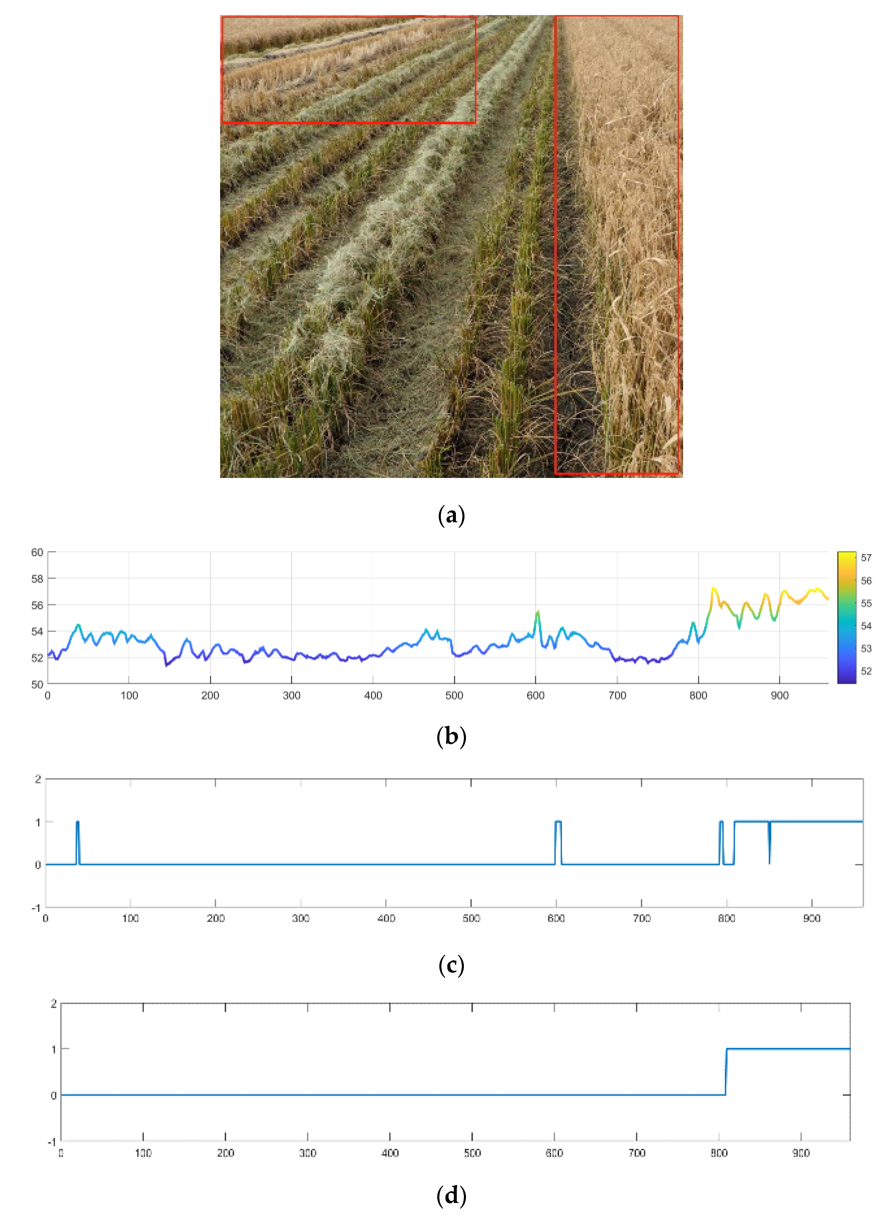
If there were two uncut areas at the far end of the image (Figure 4a), the area to be processed needed to be selected. According to the prior conditions, there was only one cut-edge at the near end of the image, which could be used to decide whether the uncut area was on the left or the right side. Then, the crop rows at the far end were selected. Both the bottom and the top of the image were vertically projected. Since it was not a necessity to do an accurate selection of the target edge, which could be included in an approximate region, the number of projection rows was set to 100 to meet the need of reducing the effect of noise.
Figure 4b shows the result gained from the projection of the bottom, which, after shaping, turned into those data illustrated in Figure 4c. A threshold value of 20 was set according to experience to eliminate noise. Figure 4d shows the result when shorter fluctuations with periods less than 20 are removed. This method can separate cut/uncut areas.
The near-end image was binarized through projection, shaping and noise reduction. The result showed that the uncut area was on the right side of the image. The mutation could be regarded as the near-end feature point of the cut-edge.
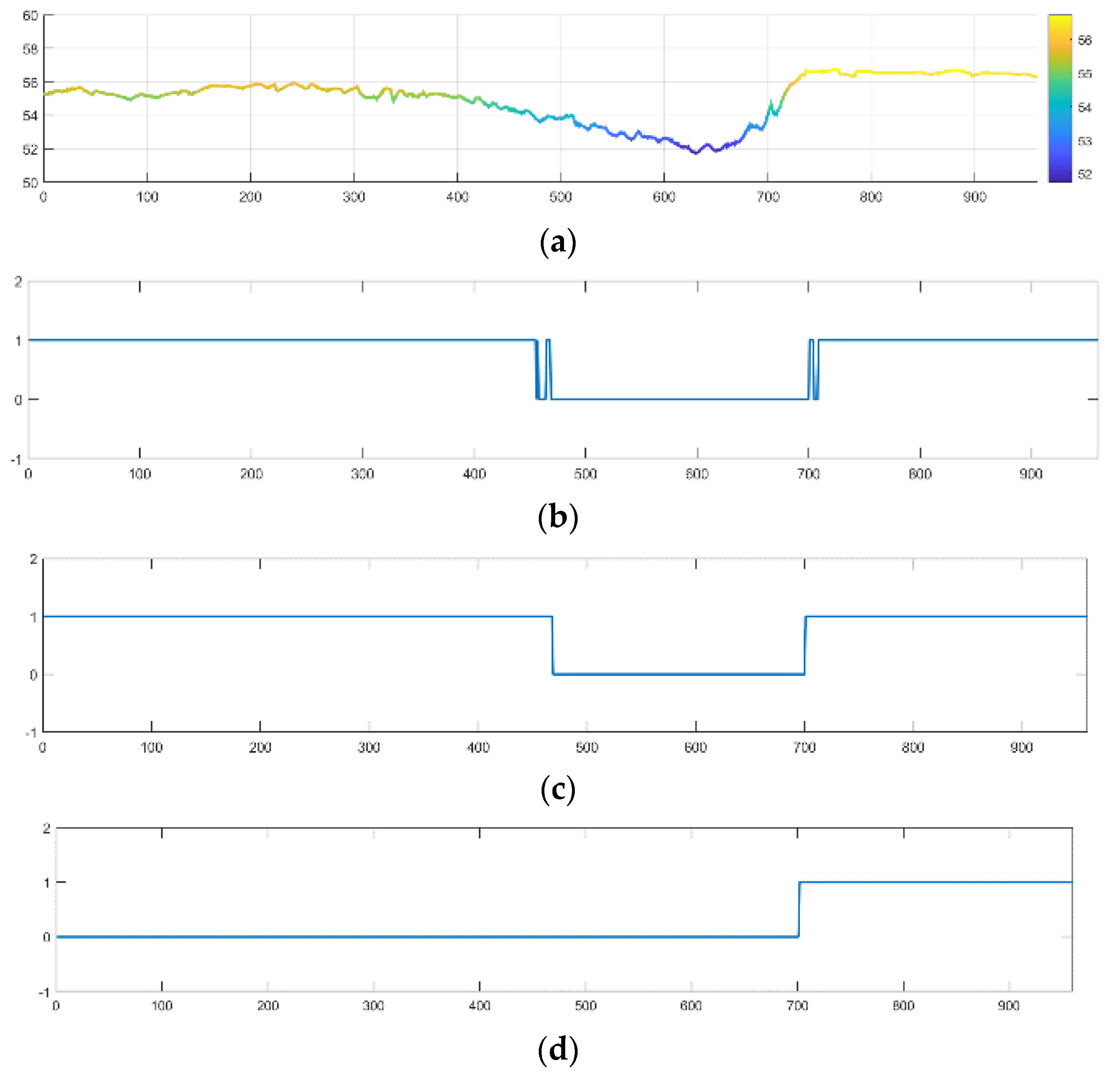
The top of the image was processed and the result was illustrated in Figure 5a–c. It showed that there were uncut areas on both sides. According to Figure 4d, the target uncut area was on the right side. The left part was set to zero, and the final result was shown in Figure 5d, which contains the feature points of the distal boundary.

2.3.3. ROI Extraction

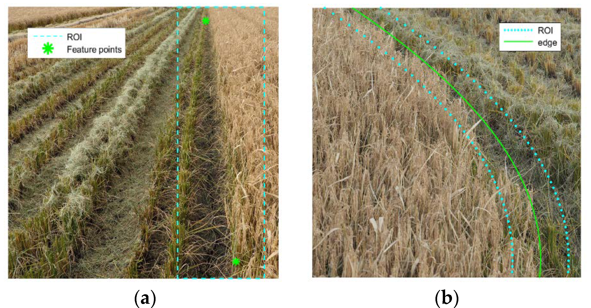
The prior conditions indicated that the cut-edge extended in one direction, so its approximate lateral range should have been between two characteristic points (Figure 6). Considering the computation and robustness, the scanning range was extended by 100 pixels (empirical value) to each side to obtain the initial ROI, as shown in the rectangular box in Figure 6a.
Because of the continuity of the field work, the difference between the two adjacent frames was small, and the frames were regarded as similar images. When the initial cut-edge was obtained, the ROI of the image was extended 100 pixels to both sides based on the cut-edge, which was taken as the ROI of the next image, as shown in Figure 6b.

2.4. Dividing Point Extraction

In this section, the dividing point was extracted in ROI in units of row. The vertical projection was used to eliminate the noise. The points in the ROI with the largest mean difference were found between the left and the right side of the image and were set as the dividing points.

2.4.1. The Vertical Projection

To eliminate the noise caused by the rice canopy texture as well as to reduce the variability within the region, it was necessary to vertically project the image according to formula (3):
P j = i 1 i i 2 P ( i , j )
P (i,j) represents the pixel value of row i, column j. The process of cumulation starts at row i1 while ends at row i2.
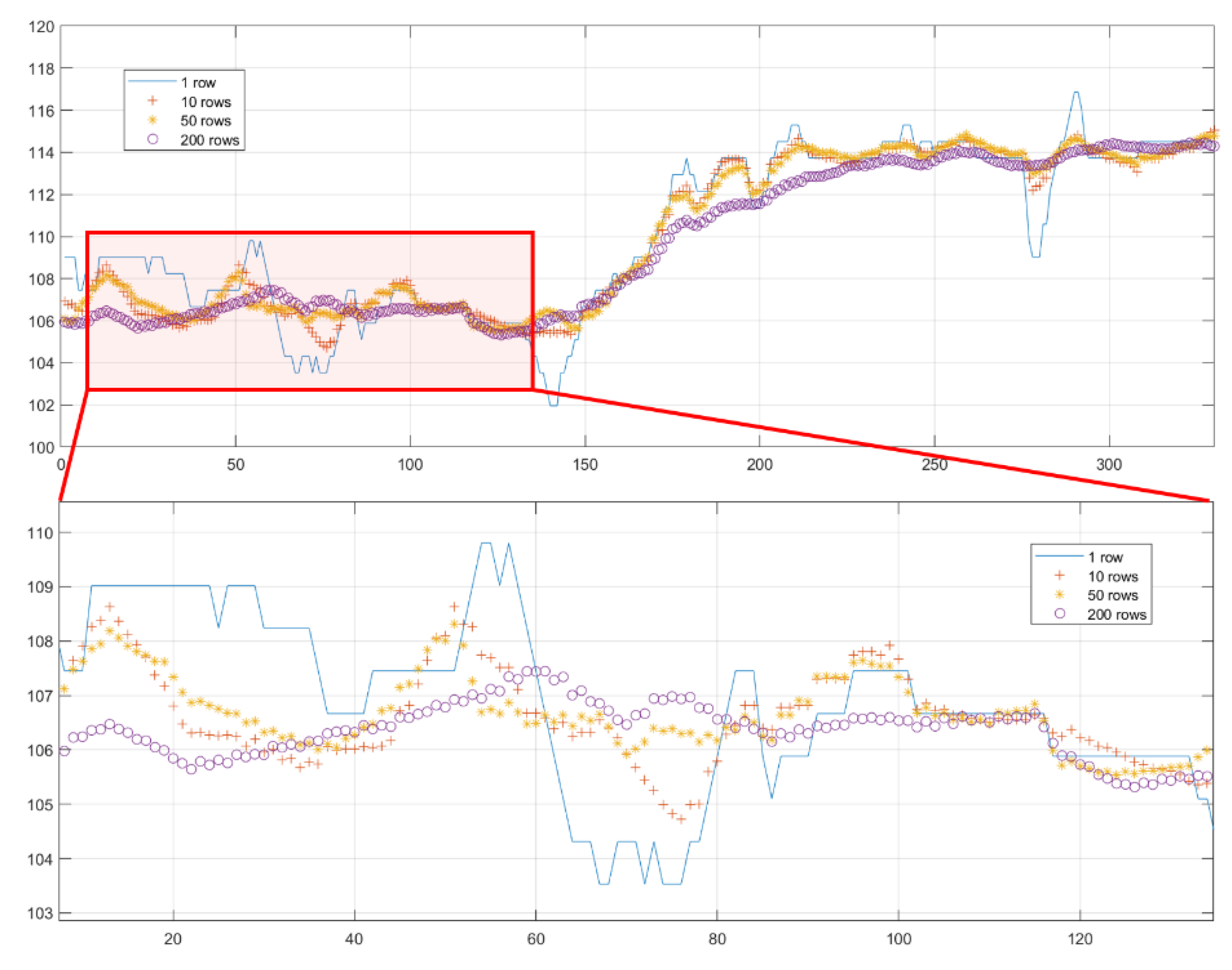
The crops were projected in 1 row, in 10 rows, in 50 rows and in 200 rows, respectively, and the results were normalized to get Figure 7. The results indicated that the uncut area was the higher part of the graph. When the number of the projected rows climbed, the consistency of the cut area increased accordingly, while the accuracy was reduced. The number of projected rows was therefore set to 10 to realize the trade-off between the computational cost and the accuracy of discrimination.

2.4.2. Dividing Points Extraction

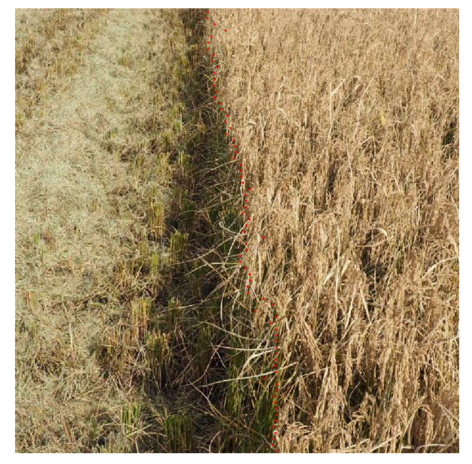
The process of extracting the dividing point was revealed in Figure 8. Projection was carried out on every 10 rows of pixels in the image. In the projection, the leftmost point within the ROI was taken. The average value of the pixels on each sides of this point were calculated, respectively. The difference between these two average values was obtained. The same calculation was applied to all points in the projection. The point with the greatest difference was the dividing point. Every 10 rows of pixels generated one dividing point, as shown in Figure 9.

2.5. Outlier Handling

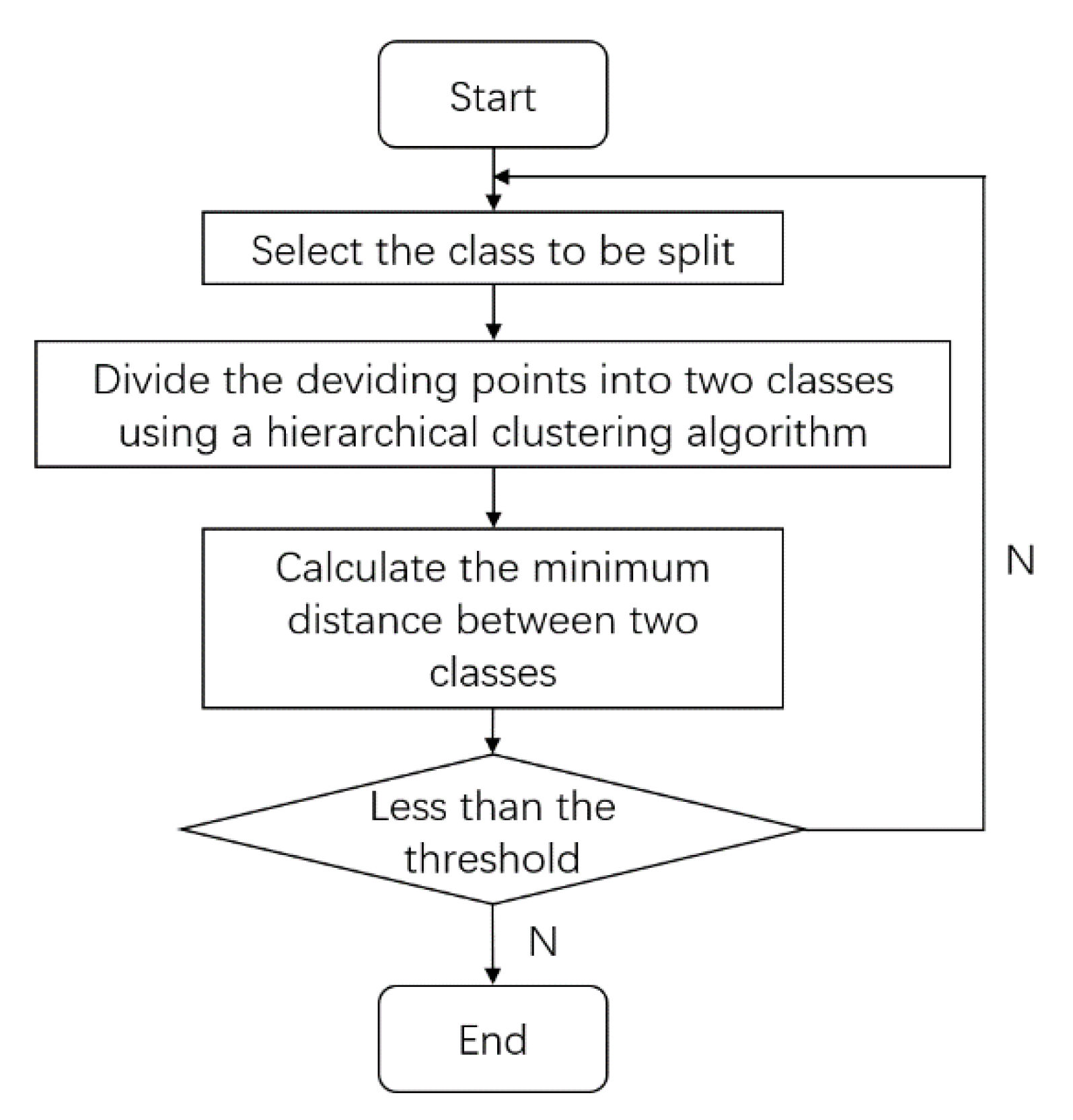
Outliers with a large offset possibly appeared in the extracted results, so they needed to be detected and corrected. In this paper, the hierarchical clustering method was adopted. A minimum distance between the clusters was taken as the classification standard. The number of categories was set as 2. After several rounds of classification, all the outliers were separated.
The classification process is shown in Figure 10. During one process, a part of outliers could be extracted. The minimum distance between these outliers and the rest ones was calculated. The calculation did not stop until the value gained from the above process was less than the threshold. The distances between the normal points in the 20 images, which as revealed by the results, were always less than 50 pixels. Therefore, the threshold was set to 50.
Piecewise linear interpolation was carried out after removing the outliers. If the outliers were at the head or the end, the closest point was taken as the modified value of it.
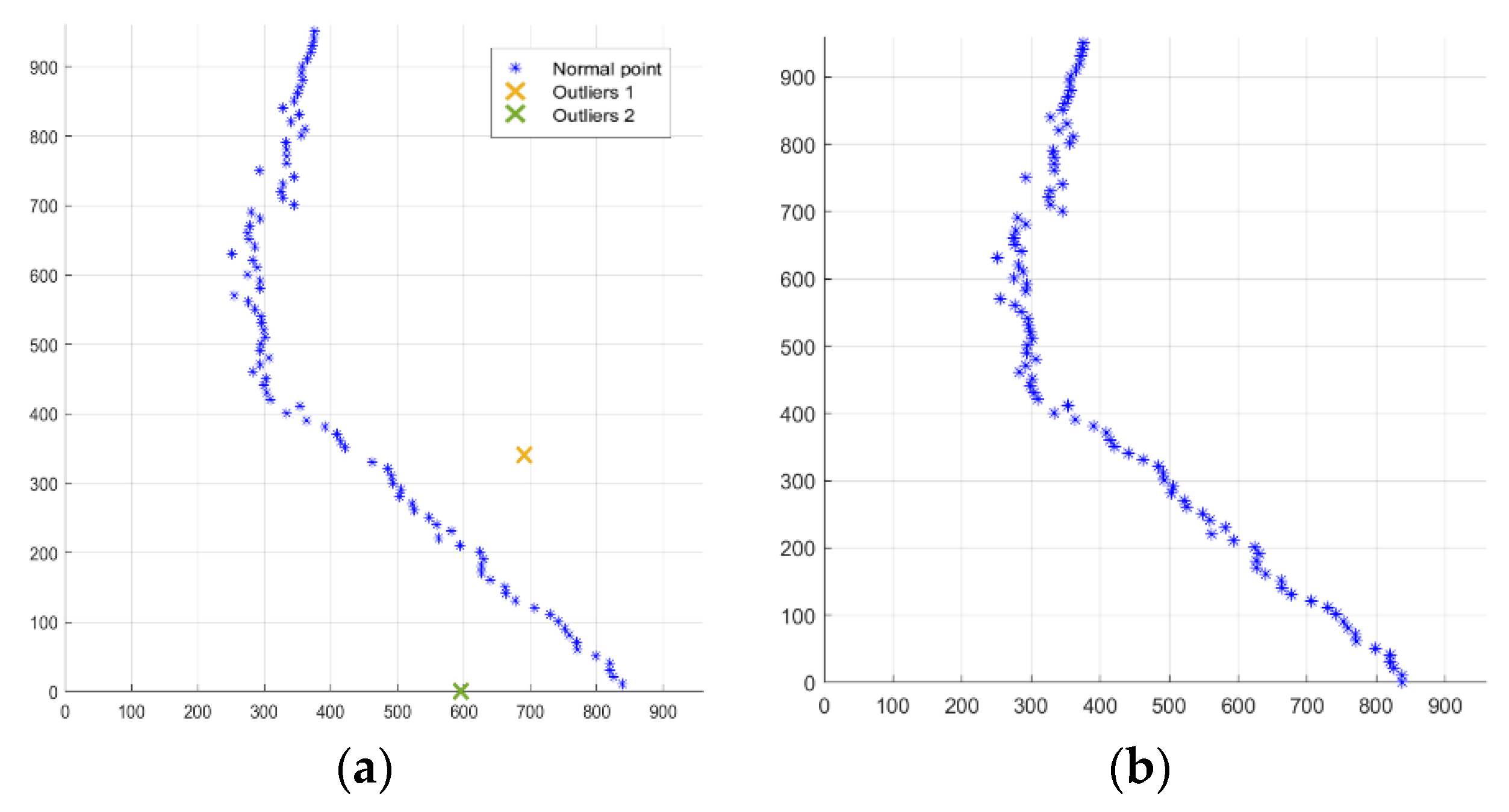
Figure 11a shows two outliers gained from two processes of classification, which were represented as outlier 1 and outlier 2. Figure 11b shows the effect when the two outliers were corrected.

2.6. Edge Fitting

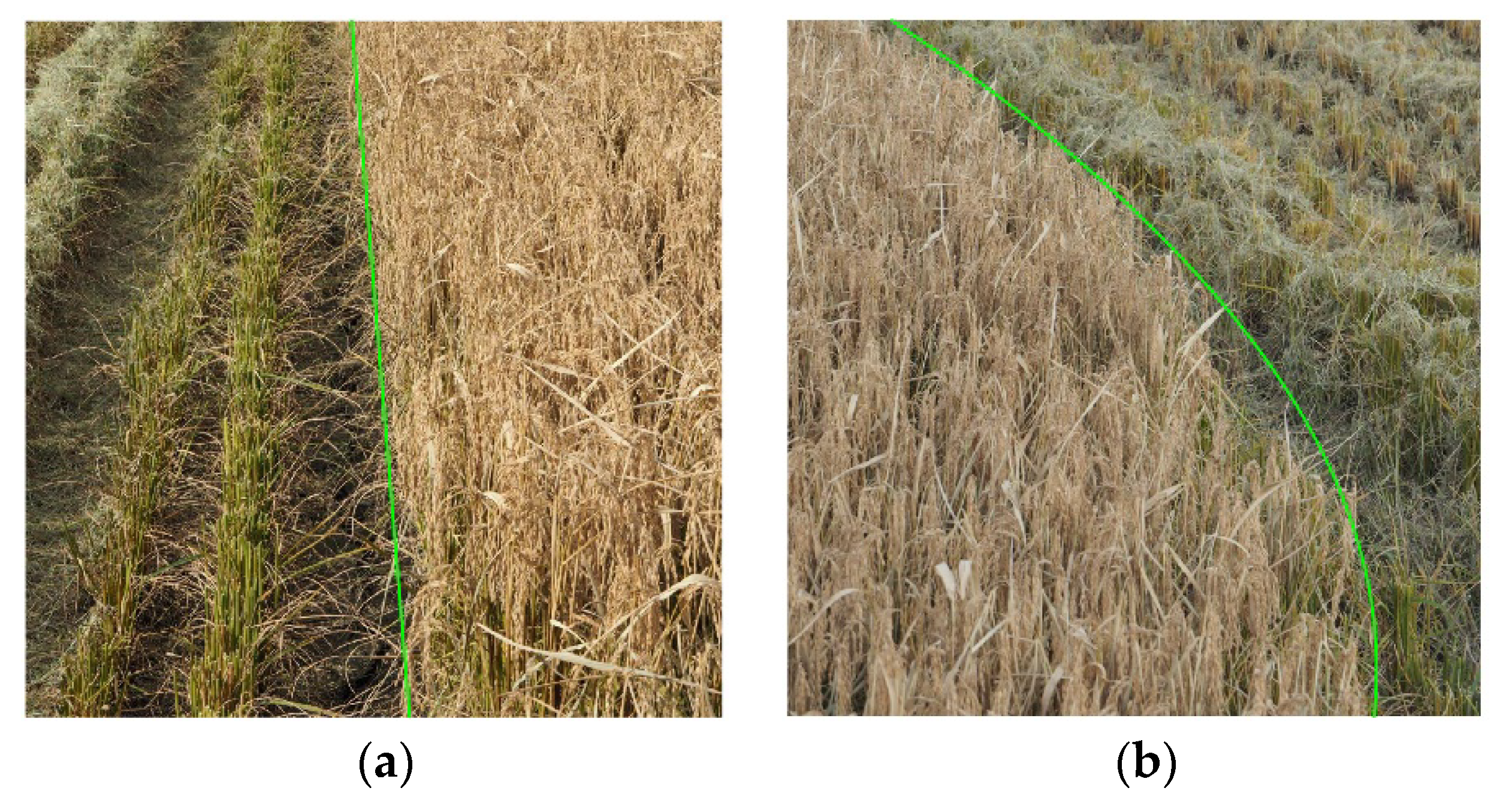
The results gained from the detection of the edge were fitted by the linear polynomial. If the R2 was higher than 0.95, then the cut-edge could be regarded as a straight line. In this situation, the linear polynomial method was applied to describe the cut-edge. Otherwise, the quadratic polynomial method was adopted. The fitting effect is shown in Figure 12.

3. Results

The image collection system was installed on the combine harvester. The images were collected in the Erdaohe Farm in Heilongjiang Province, China. The rice fields were located at 134.124679 degrees east for longitude and 47.801431 degrees north for latitude. The driver manually drove the combine harvester. Vision sensors continuously collected images during the harvest. The working speed of the combine harvester was basically maintained at 1m/s.

3.1. Grayscale Feature Factor Comparison

The components of the cut and uncut areas in 20 images were normalized to calculate the variation coefficient of the two areas and the ratio of mean. The results are shown in Table 2. The Cr component in the YCbCr color space was characterized by the feature that its intra-regional variability was relatively low while its inter-regional difference was relatively high.

3.2. ROI Extraction

The ROI extraction experiment was carried out on 100 images. The success rate was 96%. The failure was caused by the inaccurate location of the end of the row.

3.3. Dividing Points Extraction

Twenty images were extracted for the dividing points. The deviation was calculated by comparing the manually marked dividing point with the predicted point. The error statistics for locating the cut-edge of one of the images are shown in Figure 13.
The formula (4) was adopted to convert the points [Xc, Yc, Zc] in the visual coordinate system into the points [X, Y, Z] in the world coordinate system. In this formula, θ is the angle between the camera and the horizontal plane and h is the height from the center of the camera to the ground:
[ X Y Z ] = [ 1 0 0 0 s i n θ c o s θ 0 c o s θ s i n θ ] · [ X c Y c Z c ] + h [ 0 0 1 ]
According to the formula, the error in pixels is turned into an error in centimeters and the standard deviation of the error is calculated. The statistical results gained from 20 images are shown in Table 3.

3.4. Outliers Detection

Twenty images with outliers were selected for clustering. According to the manual statistics, 110outliers were identified from 116 outliers in 20 images. The recall for outliers was 94.8%.

3.5. Cut Edge Fitting

The dividing points were fitted by the linear polynomial first. If the R2 was higher than 0.95, then the cut-edge could be regarded as a straight line, and the calculation stopped. Otherwise, the cut-edge was regarded as a curved one and the quadratic polynomial fitting was applied. The fitting test was repeatedly carried out on 100 images, and the results are shown in Table 4.

4. Discussion

The extraction of the ROI removed the interference of the non-targeted areas, trees and other factors in the distance. The Cr component of the YCbCr color model diminished the impact of the shadows and illumination changes. The vertical projection reduced the noise caused by the canopy holes between the plants. Under the prior conditions, the extraction of the ROI and the dividing points, the detection of the outliers as well as the fitting of the cut-edge were all realized.
Through analyzing the results, the main reason for the failure of the ROI extraction was the inaccurate judgment of the end of the row, which prevented the interference factors from being completely removed. Moreover, the error in the extraction of the dividing points was mainly caused by the interference of the spikes protruding near the cut-edge. The reason for the error of the outlier extraction was that the fixed threshold was incapable of handling all the outliers. Therefore, to maintain a certain precision, the threshold could not be set too low, which consequently, led to the result that 5.2% of the outliers were not being detected. Through applying the linear and quadratic polynomials, the R2 of 97% of the cut-edges could reach more than 0.95. This indicated that it is advisable to use the linear and quadratic polynomials to describe most of the cut-edges.
The current method still has some inadequacy. First, the adopted method only compared the effect of the single component while the optimal combination of different components was not studied. The components will therefore be combined in different ways to find a relatively ideal combination, so that the contrast between the cut and uncut areas will be improved. Then, the negative impacts caused by shadows were not completely evaded. The failure of the extraction existed when the shadows covered too large an area. This shortcoming can be solved with a shadow removal method for rice fields. The method will be used to diminish the impact of the shadow when the shadow area is large. Finally, if the interference factor exists at the near end of the image then it cannot be eliminated. To improve robustness, the process of detecting obstacles can be added to remove near-end interference factors.

5. Conclusions

A cut-edge detection method based on machine vision was developed and evaluated under both laboratory and field conditions. The Cr component in the YCbCr color model was selected as the grayscale characteristic factor. In this way, the contrast between the cut and uncut areas was improved. This article also presented a method for automatically extracting the ROI, the success rate of which was 96%. A method to extract the dividing point was also presented, with an average error of 2.84 cm from the samples. The hierarchical clustering method was used to extract the outliers and the recall was 94.8%. The results show that the method is capable of providing support for the automatic navigation of a combine harvester.

Author Contributions

Data curation, Z.Z., R.L. and Y.S.; Investigation, Z.Z., H.L.; Methodology, Z.Z.; Software, Z.Z. and R.C.; Validation, Z.Z.; Visualization, Z.Z. and C.P.; Writing–Original draft, Z.Z.; Writing–Review & editing, M.Z. All authors have read and agreed to the published version of the manuscript.

Funding

This work was supported by the National Key Research and Development Program (Grant No.2017YFD0700400-2017YFD0700403).

Conflicts of Interest

The authors declare no conflict of interest.

References

  1. Dong, Z.Z.; Duan, J.; Wang, M.L.; Zhao, J.B.; Wang, H. On Agricultural Machinery Operation System of Beidou Navigation System. In Proceedings of the 2018 IEEE 3rd Advanced Information Technology, Electronic and Automation Control Conference, Chongqing, China, 12–14 October 2018; pp. 1748–1751. [Google Scholar]
  2. Bechar, A.; Vigneault, C. Agricultural robots for field operations: Concepts and components. Biosyst. Eng. 2016, 149, 94–111. [Google Scholar] [CrossRef]
  3. Chen, J.; Yang, G.J.; Xu, K.; Cai, Y.Y. On Research on Combine Harvester Positioning algorithm and Aided-navigation System. In Proceedings of the International Conference on Advances in Mechanical Engineering and Industrial Informatics, Zhengzhou, China, 11–12 April 2015; pp. 848–853. [Google Scholar]
  4. Long, N.B.; Wang, K.W.; Cheng, R.Q.; Yang, K.L.; Bai, J. Fusion of Millimeter wave Radar and RGB-Depth sensors for assisted navigation of the visually impaired. In Proceedings of the Conference on Millimeter Wave and Terahertz Sensors and Technology XI, Berlin, Germany, 10–11 September 2018. [Google Scholar]
  5. Yayan, U.; Yucel, H.; Yazici, A. A Low Cost Ultrasonic Based Positioning System for the Indoor Navigation of Mobile Robots. J. Intell. Robot. Syst. 2015, 78, 541–552. [Google Scholar] [CrossRef]
  6. Zampella, F.; Bahillo, A.; Prieto, J.; Jimenez, A.R.; Seco, F. Pedestrian navigation fusing inertial and RSS/TOF measurements with adaptive movement/measurement models: Experimental evaluation and theoretical limits. Sens. Actuators A Phys. 2013, 203, 249–260. [Google Scholar] [CrossRef]
  7. Ball, D.; Upcroft, B.; Wyeth, G.; Corke, P.; English, A.; Ross, P.; Patten, T.; Fitch, R.; Sukkarieh, S.; Bate, A. Vision-based Obstacle Detection and Navigation for an Agricultural Robot. J. Field Robot. 2016, 33, 1107–1130. [Google Scholar] [CrossRef]
  8. Hacioglu, A.; Unal, M.F.; Altan, O.; Yorukoglu, M.; Yildiz, M.S. Contribution of GNSS in Precision Agriculture. In Proceedings of the 8th International Conference On Recent Advances in Space Technologies, Istanbul, Turkey, 19–22 June 2017; pp. 513–516. [Google Scholar]
  9. Malavazi, F.B.P.; Guyonneau, R.; Fasquel, J.B.; Lagrange, S.; Mercier, F. LiDAR-only based navigation algorithm for an autonomous agricultural robot. Comput. Electron. Agric. 2018, 154, 71–79. [Google Scholar] [CrossRef]
  10. Mark, O.; Anthony, S. First Results in Vision-Based Crop Line Tracking. In Proceedings of the Robotics & Automation, Minneapolis, MN, USA, 22–28 April 1996; pp. 951–956. [Google Scholar]
  11. Mark, O.; Anthony, S. Vision-Based Perception for an Automated Harvester. In Proceedings of the Intelligent Robots and Systems, Grenoble, France, 8–13 September 1997; pp. 1838–1844. [Google Scholar]
  12. Debain, C.; Chateau, T.; Berducat, M.; Martinet, P. A Guidance-Assistance System for Agricultural Vehicles. Comput. Electron. Agric. 2000, 25, 29–51. [Google Scholar] [CrossRef]
  13. Benson, E.R.; Reid, J.F.; Zhang, Q. Machine Vision-based Guidance System for Agricultural Grain Harvesters using Cut-edge Detection. Biosyst. Eng. 2003, 86, 389–398. [Google Scholar] [CrossRef]
  14. Cornell University Library, eCommons. Available online: https://ecommons.cornell.edu/handle/1813/10608 (accessed on 11 July 2007).
  15. Zhang, L.; Wang, S.M.; Chen, B.Q.; Zhang, H.X. Crop-edge Detection Based on Machine Vision. N. Z. J. Agric. Res. 2007, 50, 1367–1374. [Google Scholar]
  16. Michihisa, I.; Yu, I.; Masahiko, S.; Ryohei, M. Cut-edge and Stubble Detection for Auto-Steering System of Combine Harvester using Machine Vision. IFAC Proc. Vol. 2010, 43, 145–150. [Google Scholar]
  17. Ding, Y.C.; Chen, D.; Wang, S.M. The Mature Wheat Cut and Uncut Edge Detection Method Based on Wavelet Image Rotation and Projection. Afr. J. Agric. Res. 2011, 6, 2609–2616. [Google Scholar]
  18. Zhang, T.; Xia, J.F.; Wu, G.; Zhai, J.B. Automatic Navigation Path Detection Method for Tillage Machines Working on High Crop Stubble Fields Based on Machine Vision. Int. J. Agric. Biol. Eng. 2014, 7, 29–37. [Google Scholar]
  19. Wonjae, C.; Michihisa, L.; Masahiko, S.; Ryohei, M.; Hiroki, K. Using Multiple Sensors to Detect Uncut Crop Edges for Autonomous Guidance Systems of Head-Feeding Combine Harvesters. Eng. Agric. Environ. Food 2014, 7, 115–121. [Google Scholar]
  20. Cornell University Library. Available online: https://arxiv.org/abs/1501.02376 (accessed on 10 January 2015).
  21. Kneip, J.; Fleischmann, P.; Berns, K. Crop Edge Detection Based on Stereo Vision. Intell. Auton. Syst. 2018, 123, 639–651. [Google Scholar]
  22. Kise, M.; Zhang, Q.; Mas, F.R. A Stereovision-based Crop Row Detection Method for Tractor-automated Guidance. Biosyst. Eng. 2005, 90, 357–367. [Google Scholar] [CrossRef]
  23. Kebapci, H.; Yanikoglu, B.; Unal, G. Plant Image Retrieval Using Color, Shape and Texture Features. Comput. J. 2011, 54, 1475–1490. [Google Scholar] [CrossRef] [Green Version]
  24. Garcia-Santillan, I.; Guerrero, J.M.; Montalvo, M.; Pajares, G. Curved and Straight Crop Row Detection by Accumulation of Green Pixels from Images in Maize Fields. Precis. Agric. 2018, 19, 18–41. [Google Scholar] [CrossRef]
  25. Rohit, M.; Ashish, M.K. Digital Image Processing Using SCILAB; Springer: Berlin, Germany, 2018; pp. 131–142. [Google Scholar]
  26. Shiva, S.; Dzulkifli, M.; Tanzila, S.; Amjad, R. Recognition of Partially Occluded Objects Based on the Three Different Color Spaces (RGB, YCbCr, HSV). 3D Res. 2015, 6, 22. [Google Scholar]
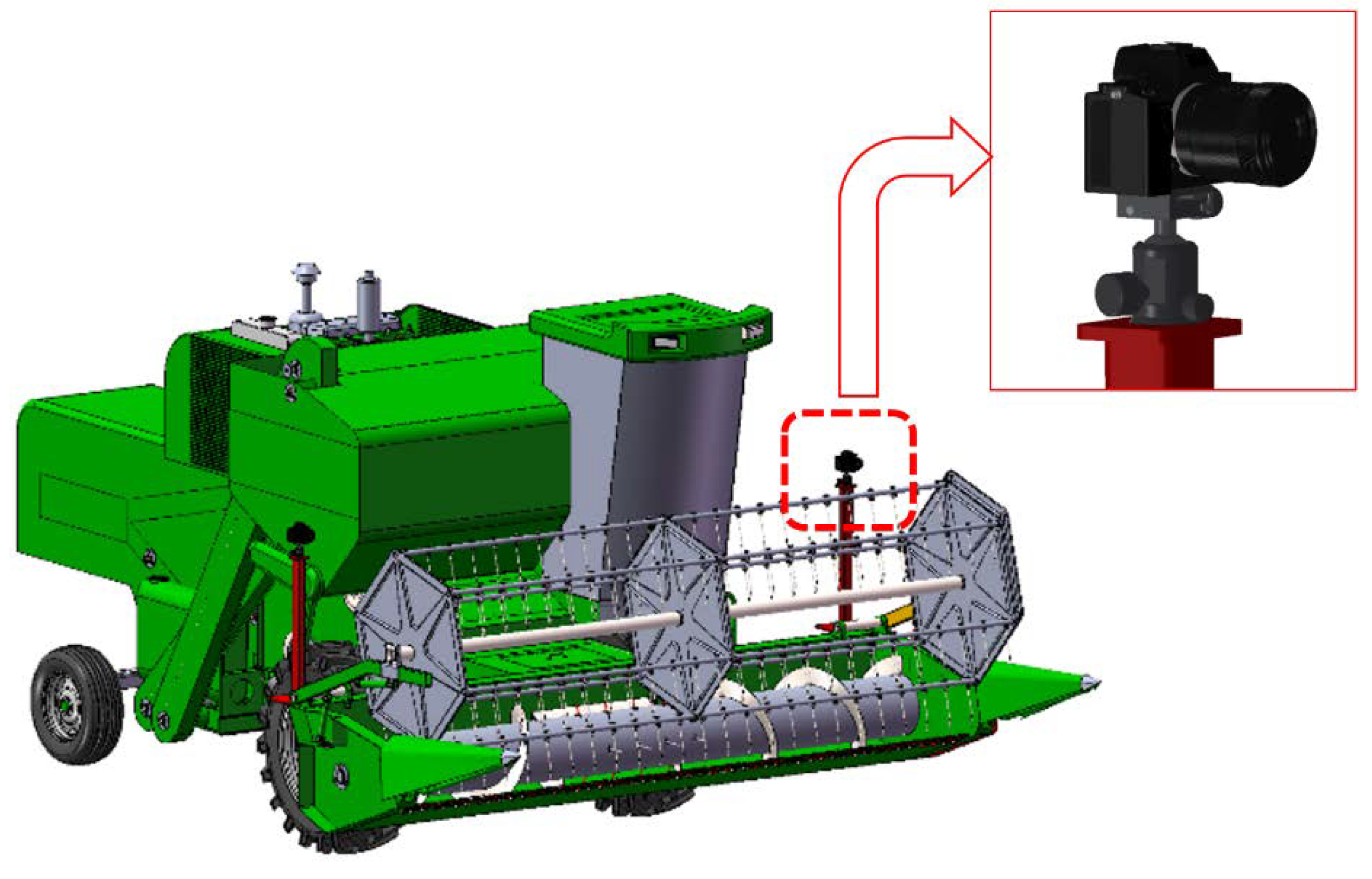
Figure 1. Camera mounting structure.
Agronomy 10 00590 g001
Figure 2. Figure of each color space component model: (a) RGB image; (b) HSV model; (c) NTSC model; (d) YCbCr model.
Agronomy 10 00590 g002
Figure 3. Horizontal projection results: (a) Image to be extracted; (b) Horizontal projection results; (c) Shaped results; (d) Preserved area of interest; (e) Extracted results.
Agronomy 10 00590 g003
Figure 4. Target crop row selection process: (a) Image to be processed; (b) Projected results; (c) Results after shaping; (d) Noise reduction results.
Agronomy 10 00590 g004
Figure 5. Top processing results of the image: (a) Projection results; (b) Shaped results; (c) Noise reduction results; (d) Selected results.
Agronomy 10 00590 g005
Figure 6. Region of interest (ROI) extraction results: (a) Initial ROI extraction; (b) Dynamic ROI extraction.
Agronomy 10 00590 g006
Figure 7. Number of different projection lines.
Agronomy 10 00590 g007
Figure 8. Dividing point extraction process.
Agronomy 10 00590 g008
Figure 9. Dividing point extraction effect.
Agronomy 10 00590 g009
Figure 10. Outlier extraction process.
Agronomy 10 00590 g010
Figure 11. Exception extraction and correction: (a) Outliers detection results; (b) Exception correction results.
Agronomy 10 00590 g011
Figure 12. Dividing point fitting effect: (a) Straight cut-edge; (b) Curved cut-edge.
Agronomy 10 00590 g012
Figure 13. The error statistics of an image.
Agronomy 10 00590 g013
Table 1. Current research status of the harvester vision navigation.
MethodCropReference
Color segmentationAlfalfa hayM. Ollis [10,11], 1996
Texture segmentationGrassC. Debain [12], 2000
Grayscale segmentationCornE.R. Benson [13], 2003
Stereo vision detectionCornF. Rovira-Más [14], 2007
Luminance segmentationWheat, cornZ. Lei [15], 2007
Grayscale segmentationRiceM. Iida [16], 2010
Wavelet transformationWheatY. Ding [17], 2011
Color segmentationWheat, rice, rapeseedZ. Tian [18], 2014
Color segmentationRiceW. Cho [19], 2014
Color segmentationWheatM.Z. Ahmad [20], 2015
Point cloud segmentationWheat, rapeseedJ. Kneip [21], 2020
Table 2. Comparison of the different components.
Grayscale Feature FactorVariation Coefficient of Cut AreaVariation Coefficient of Uncut AreaRatio of Mean
HSV-H0.22630.09740.8441
HSV-S0.37780.30110.9291
NTSC-I0.04630.03580.924
NTSC-Q0.03910.01720.9844
YCbCr-Cb0.05990.03460.9443
YCbCr-Cr0.02350.01890.9169
Table 3. Results of the dividing points extraction.
IndexError in PixelsError in CentimetersStandard Deviation
value4.722.8418.49
Table 4. Result of the edge fitting.
Fit MethodLinear Polynomial R² > 0.95Quadratic Polynomial R² > 0.95Quadratic Polynomial 0.75 < R² < 0.95
Amount82153