Data Grouping Method for the Purpose of Forecasting the Mechanical Strength of Plastic Soils

Abstract

The aim of this work was to develop a method of data grouping (DGM) that enables the selection of regression equations for forecasting soil penetration resistance based on an easily available and small set of input data: soil moisture content, soil bulk density and the grain size distribution of the soil. Models for forecasting the penetration resistance were created by selecting regression equations for specific intervals of granulometric variability of soil fractions. A field measurements campaign was conducted and soil samples were taken from the subsoil on 43 profiles, at depths of 25–30, 35–40, 45–50 and 55–60 cm. It was found that the dry bulk density is much less useful for predicting the penetration resistance of plastic soils than soil moisture. The study also showed that it is possible to forecast the soil penetration resistance on the basis of the gravimetric moisture content and the soil specific surface.

1. Introduction

Excessive compaction of soils by wheels of machines and vehicles is one of the most serious agricultural problems, which has been known about for years [1]. Soil compaction can cause adverse changes in soil properties leading to the disappearance of aggregate structure, reduction of water and air conductivity, reduction of water retention, etc. These adverse changes result in reduction in crops [2], increase of production costs [3], and increase of environmental threats [4]. The soils particularly susceptible to compaction include heavy loams, clays, and light loams [5]. Especially dangerous is the excessive compaction of the subsoil, because the effects are long-lasting and attempts to loosen the soil are energy-consuming, often ineffective, and in some soil and atmospheric conditions may cause greater losses than benefits [6].

The subsoil compaction increases when the soil strength is exceeded. The soil compaction strength may be characterized by using various indicators, such as penetration resistance (PR) among others. The resistance to penetration is called the cone index when divided by the cone base surface area. This method is relatively easy and quick to use.

Comparing the PR with other soil properties, including other strength properties, makes knowledge of the penetration resistance value practical. The PR value indirectly allows one to determine, for example: the soil pre-compression stress [7], the draught force of tillage implements, vehicle trafficability and the growth (or elongation rate) of plant roots in the soil [8,9,10]. From the point of view of soil protection against excessive compaction, it is important to know the soil pre-compression stress. Information on the soil pre-compression stress along with the distribution of stresses from the pressures exerted on the surface can predict the load of tractors’ or machines’ running gears [11].

There is a need to be able to predict penetrometric resistance from basic soil properties such as the soil composition, bulk density and water content [8,12,13,14]. It is generally found that for any one soil, it is quite easy to produce an empirical equation that accounts for differences in bulk density and water content. However, the predictions are often not so good when different soils are being compared [8]. Therefore, the empirical mathematical models to predict the pre-compression of the soil are created by selecting the regression equations for a given range of variability of the soils researched [15,16]. The determination of the ranges of the variability of the soils requires an assumption of their grouping (classification). It may be noted that it is not advisable to use the symbols of the marked soil grades for this purpose. This is because the currently used systems classify the soil formations on the basis of their graining and therefore could possibility include significantly different soils in the same granulometric group or could place almost identical soils into different groups [17,18].

The aim of the work was to develop the method of soil data grouping (DGM) enabling the selection of regression equations to predict penetrometric resistance. Models that were useful in practice were sought, enabling estimation of the current value of penetrometric resistance on the basis of an easily available and small set of input data, the acquisition of which does not require complicated experimental research. A simplifying assumption was made that the strength of soils with similar intrinsic properties depends on soil moisture and bulk density. This approach allows one to omit other factors that affect penetrometric resistance, e.g., soil depths, soil type, sampling time etc. Due to the fact that it is difficult to choose the same prognostic model for cultivated and uncultivated soil [19], the research was limited to the subsoil layer of soils.

In view of the huge number of factors affecting the physical-mechanical properties of soils, modeling of strength properties is an extremely difficult task. In order to eliminate unrecognized mutual interactions of various factors on soil strength, a staged method of iteration to divide the studied soils into groups was applied in a way that would eliminate disturbances caused by unrecognized natural soil variability.

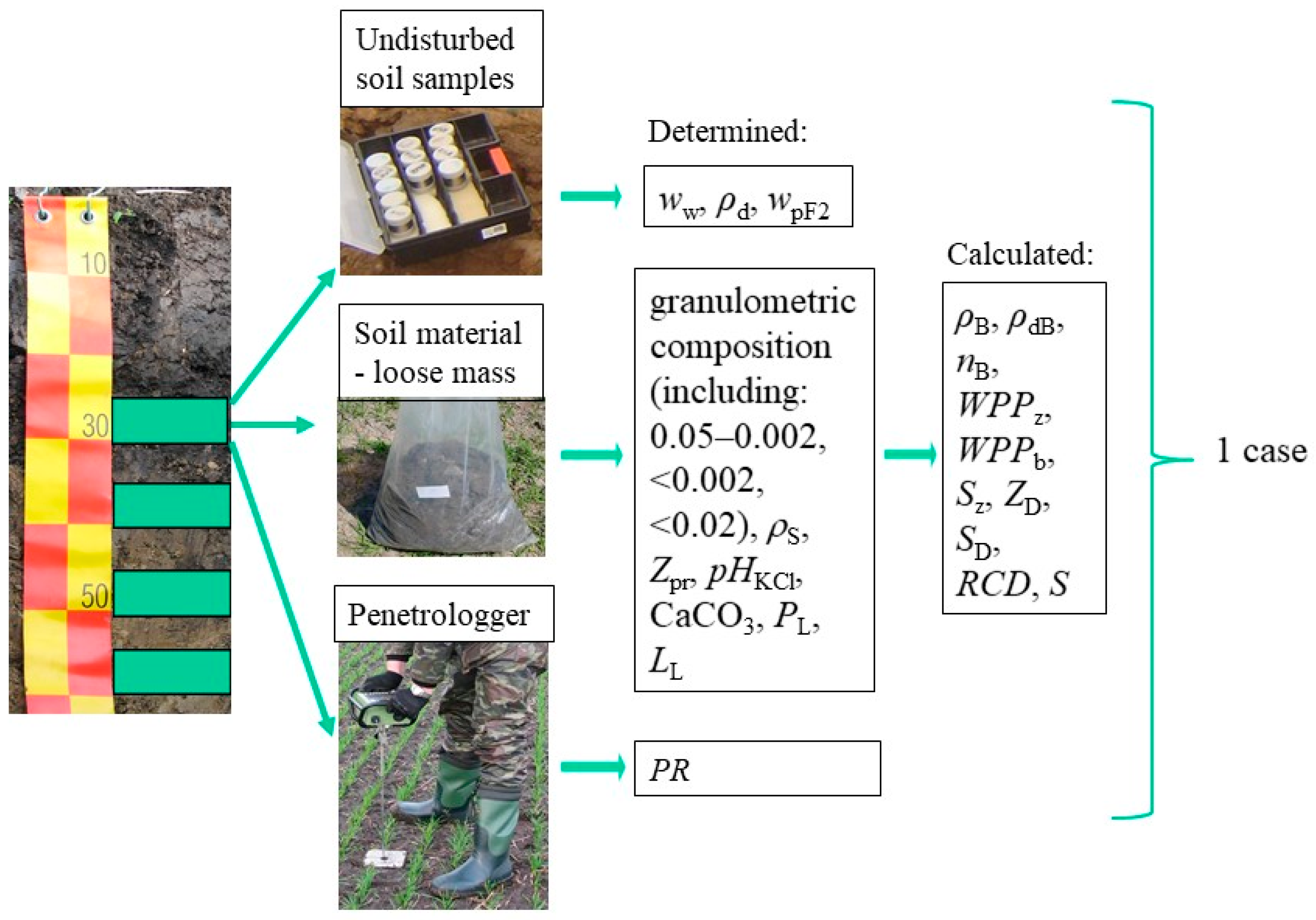
2. Materials and Methods

The study consisted of the following stages: collecting a large set of data, developing the method of soil data grouping, selecting regression equations for PR forecasting and assessing them. These stages are described in detail below (Figure 1).

2.1. The Characteristic of the Researched Soils

The development of the data grouping method started with the collection of experimental data. Experiments were performed on plastic soils of the Szczecin Lowland, north-west Poland. Soil material was taken from 13 sites. On each site, 1 or 4 profiles of soil pits were described, in which the first planned measurements were carried out—a total of 43 profiles. In the following years, measurements were repeated in soil pits, 2 to 3 m apart from each of the previously described profiles—a total of 57 pits. The measurements were carried out in the spring time (24 March–10 May) and in autumn (27 September–14 December), in a non-tilled sub-soil layer, at depths of 25–30, 35–40, 45–50 and 55–60 cm. In the sites where ploughing was performed to a depth of 30 cm, a layer of 25–30 cm was omitted.

The time of performing field measurements and taking soil samples for laboratory tests was dependent on the soil moisture [20]. Undisturbed soil samples were collected using cylinders of 50 mm high and 50 mm diameter. Each sample was protected against moisture loss during transport by fitting the protective covers over the sample rings. For each of the soil layers in each soil pit, 4 samples were used to determine: the soil gravimetric moisture content (w_w), the dry bulk density (ρ_d) and the soil moisture at pF2 (w_pF2), using a gypsum board. The w_pF2 was determined in order to assess soil moisture at the time of PR measurement. The w_w and w_pF2 and density ρ_d of the soil were determined by a drying-weight method (oven-dried at 105 °C for 24 h). The PR was measured with a cone of 30° angle and a base area of 1 cm², using the Penetrologger made by the Eijkelkamp company, the Netherlands. The penetration rate was 2 cm·s⁻¹. The measurements of the PR were repeated 10 times for each soil layer in each soil pit.

The granulometric composition was determined by the Bouyoucos-Casagrande method modified by Prószyński [21]. The pycnometric method was used to determine the density of the solid particles (ρ_s), using the pycnometer G-L (100 cm³) made by the WPL Gliwice company (Poland). The humus content (Z_pr) was determined with the use of the Tiurin method and the pH reaction of the soil (pH_KCl)—by means of the electrometric method. The calcium carbonate content (CaCO₃) was determined by the Scheibler method. The plastic limit (P_L) and the liquid limit (L_L) according to Atterberg were determined. Data of the characteristics of the soil itself are presented in the Appendix A (

Table A1. Ranges of properties of researched soils for individual sites in layer of 25–60 cm.

Site Designation	ρs	pHKCl	Zpr	CaCO3	PL	LL	Content of Fraction			Soil Texture Acc. USDA [29]
							0.05–0.002	<0.002	<0.02
	(g·cm–3)	(–)	(%)		(% w/w)		(%)
Cz	2.49–2.79	6.36–6.91	0.33–1.41	–	14.4–23.7	23.3–49.0	24.7–40.9	11.4–26.8	36–60	SL, SCL, L,
De	2.46–2.67	5.55–7.50	0.38–1.83	–	15.3–26.6	19.8–50.5	33.6–56.6	9.9–34.7	25–68	SiL, SL, CL, L
Ku	2.55–2.73	6.33–7.06	0.21–1.06	0.00–0.13	11.6–26.7	12.7–46.2	15.7–37.1	5.9–31.3	20–59	SL, SCL, CL, L
Sł	2.46–2.54	5.46–5.93	0.83–1.52	–	16.5–17.9	20.4–23.0	36.0–40.3	7.8–9.8	23–27	L, SL
Lu	2.55–2.71	7.53–7.85	0.32–1.74	0.97–11.46	13.3–19.4	16.3–30.9	28.0–41.8	11.4–20.5	31–49	SL, L
No	2.56–2.65	4.97–5.80	0.25–1.13	–	16.7–21.6	23.0–37.8	34.3–38.4	9.8–24.5	24–52	SL, L
NP	2.45–2.47	6.21–6.34	1.09–3.09	0.78–2.86	20.3–23.7	29.5–31.3	50.2–56.6	8.9–14.5	33–38	SiL
Ob1	2.40–2.67	6.52–7.18	0.75–4.17	0.00–22.18	24.9–31.4	36.1–73.0	45.7–71.6	16.9–41.8	62–91	SCL, SiL, SiC, L
Ob2	2.47–2.71	6.27–6.78	0.54–2.21	0.00–0.52	12.8–19.0	16.2–32.0	17.5–34.5	9.8–15.7	22–40	SL, L
Os	2.52–2.74	4.67–5.65	0.39–1.06	–	14.1–23.1	17.0–35.1	22.1–40.4	8.8–22.5	31–50	SL, L
Re	2.39–2.44	6.43–6.50	2.91–4.03	0.55–5.18	22.0–25.9	31.8–37.0	44.7–50.0	11.8–13.9	31–35	L
Sk	2.50–2.70	5.48–6.99	0.60–1.92	0.00–0.09	17.9–40.4	26.4–99.3	24.3–66.5	11.7–40.8	35–90	SCL, SL, SiL, L, CL, SiCL
St	2.42–2.70	6.70–7.34	0.52–4.12	0.00–0.43	15.1–23.9	22.7–31.5	27.4–36.5	12.8–19.6	29–42	SL, L

Caution: ρ_s–density of solid particles; Z_pr–humus content; CaCO3–calcium carbonate content („–” sign mans that occurrence was not found); P_L–plastic limit; L_L–liquid limit; SL–sandy loam; SCL–sandy clay loam; L–loam; SiL–silt loam; CL–clay loam; SiC–silty loam; SiCL–silty clay loam.

).

The characteristic of the soils was enlarged by the information on the properties calculated on the basis of the results of the granulometric composition and the humus content. The calculated density of solid particles (ρ_B), the calculated dry density (ρ_dB), and the general porosity (n_B) were determined with the use of the Brogowski equations [22]. The field water capacity was calculated with the use of the Trzecki [23] formulae with the participation of (WPP_z) or without the participation of the humus content (WPP_b). The method proposed by Prusinkiewicz and Proszek [24] was used to calculate the grain average diameter (S_z), the specific surface (Z_D) and the dispersion index (S_D). The content of the easily dispersing clay in the soil (RCD) was calculated in accordance with Czyż [25] on the basis of the clay content (fraction <0.002 mm) and the organic substance. The stability index (S) was estimated with the use of the Pieri equation [26] on the basis of the content of humus and the fractions of silt and clay. More details about the calculation—ρ_B, ρ_dB, n_B, WPP_z, WPP_b, S_z, Z_D, S_D, RCD and S—are given in the Appendix A.

Determined and calculated properties for each soil layer in each measurement term formed data cases (Figure 2).

Table 1. Number of profiles and pits per site, the location of arable fields of individual sites and soil cultivation depth.

Site Designation	Number of Soil Profiles	Number of Pits of the Basic Set	Number of Pits of the Validation Set	Field Located *	Soil Groups (acc. WRB-FAO)	Maximum Soil Tillage Depth **
						(cm)
CzBS	4	8	-	52° 54’ 02”N; 14° 14’ 05”E	Cambisols	18
DeBS	4	8	-	53° 15’ 20”N; 14° 58’ 04”E	Phaeozems	25
Ku	4	8	3	53° 15’ 45”N; 15° 04’ 04”E	Luvisols	25
SłVS	1		2	53° 16’ 57”N; 14° 57’ 01”E	Phaeozems	22
LuBS	4	8	-	52° 54’ 03”N; 14° 14’ 02”E	Cambisols	18
NoBS	4	8	-	54° 04’ 40”N; 15° 15’ 48”E	Cambisols	30
NPVS	1		2	53° 13’ 18”N; 15° 01’13”E	Phaeozems	22
Ob1	4	8	3	53° 09’ 59”N; 14° 55’ 19”E	Phaeozems	25
Ob2BS	4	8	-	53° 09’ 16”N; 14° 55’ 30”E	Phaeozems	30
Os	4	8	3	53° 24’ 49”N; 14° 27’ 49”E	Cambisols	15
ReVS	1		2	53° 14’ 17”N; 14° 57’ 32”E	Phaeozems	18
Sk	4	8	4	53° 26’ 27”N; 14° 25’ 48”E	Cambisols	20
St	4	8	1	53° 16’ 57”N; 14° 57’ 01”E	Phaeozems	15

*—the location given refers to the field and not the specific soil profile; **—the given cultivation depth refers to the period of two years preceding the measurements; Designations of sites—site name: Cz—Czachów, De—Dębica, Ku—Kurcewo, Sł—Słotnica, Lu—Lubiechów, No—Nowielice, NP—Nowy Przylep, Ob₁—Obojno, Ob₂—Obojno „Gospodarstwo”, Os—Ostoja, Re—Reńsko, Sk—Skarbimierzyce, St—Stobno; ^BS—data used only to form the basic set, ^VS—data used only for validation (the validation set).

gives the number of profiles and pits per site, the location of arable fields of individual sites, soil types and depth of soil cultivation. The soils were classified as a Phaeozems, Cambisols and Luvisols according to the WRB FAO system. Maximum soil tillage depth was from 15 to 30 cm. The data collected in the form of cases (data rows) was divided into two subsets: the main set (275 cases) and the validation set (77 cases), which was used to estimate the predicted error of the PR. The data obtained in the years 2003–2006 formed the basic set, and the data obtained in the years 2007–2012 constituted the validation set. The basic set is data collected from sites for which 4 profiles were described and measurements were taken in 2 repetitions—a total of 8 pits per site (Table 1). The validation set is data from sites for which one profile was described and measurements were carried out in 2 replications (sites: Sł, NP, Re). The validation set was increased by data collected from pits made in 2007–2012 (sites: Ku, Ob₁, Os, Sk, St). Every case (data row) consisted of one dependent variable (PR), two independent variables (w_w, ρ_d), and other properties describing soils, including those named grouping parameters: fractions of granulometric composition, Z_pr, P_L, L_L, ρ_B, ρ_dB, n_B, WPP_b, S_z, Z_D, S_D; RCD, S, WPP_z. The validation set was diversified in terms of soil describing properties as well as the place and depth of sampling. The set of validation data obtained this way was not used to create regression equations.

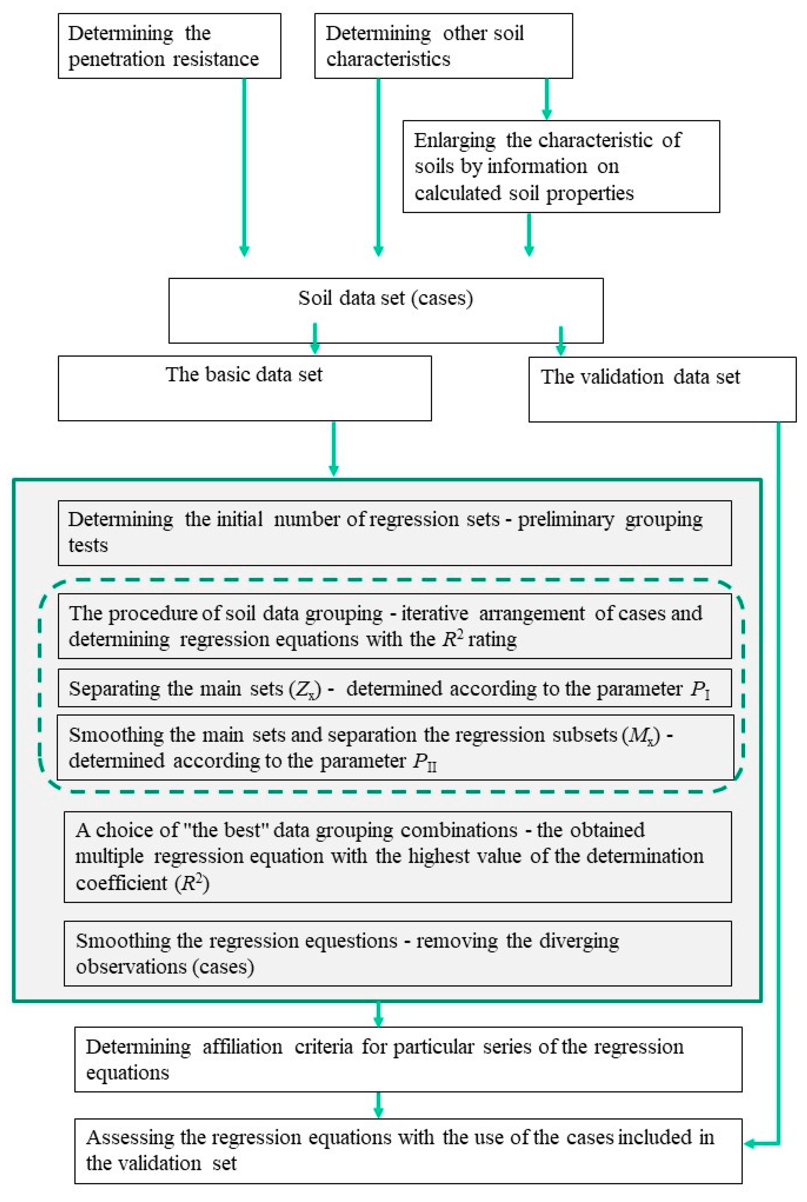
2.2. Data Grouping Method

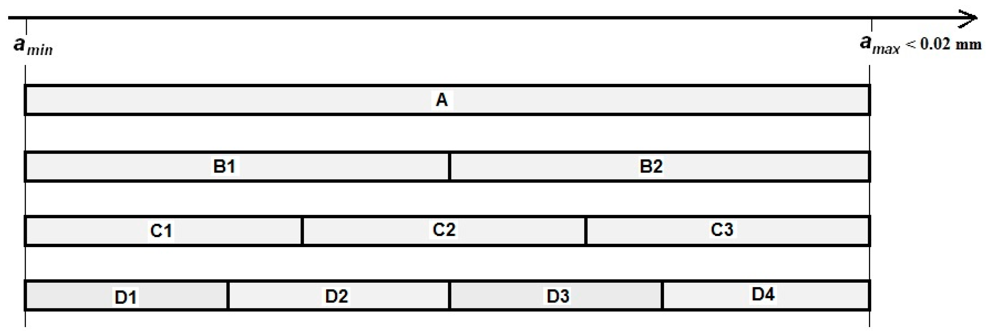
2.2.1. The preliminary Grouping Tests

The development of this method was preceded by attempts to group (stack) the observations in regards to the content of the particles <0.02 mm, their division into a various number of the sets (see Figure 3) and checking the values of the multiple regression coefficient (R²) for the dependence of the PR on the selected independent variables. Because of their widespread use, the selected variables were: the gravimetric moisture content and the dry bulk density. It was also noted that despite the importance of particle sizes, the content of the fine particles poorly distinguishes among the soils in some ranges of their variability. This is because fine particle size described only a part of the granulometric composition of the soil. Other parameters (indicators) were used to arrange the cases, which better diversified the soils. Those parameters were highly correlated with the content of fine particles and calculated on the basis of the largest possible number of the different granulometric fractions. The best result was obtained by dividing the observations (cases) into four sets (defined as quartiles). It was found that higher values of the determination coefficient could be obtained by taking into consideration the number of the cases between the quartiles 1 and 3 within each of the sets. Such a procedure caused a rejection of the cases smaller than the quartile 1 and bigger than the quartile 3. It was therefore decided that a given set should be smoothed out before the rejection, the purpose of which was to reduce the interferences resulting from the natural variability of soils. It was found a priori that such parameters used for this procedure, should correlate with the particle content <0.02 mm and be associated with the other selected soil characteristics, affecting the soil strength.

Therefore, the result of the initial grouping was to determine the initial number of data sets and to direct further work aimed at developing a procedure for grouping data.

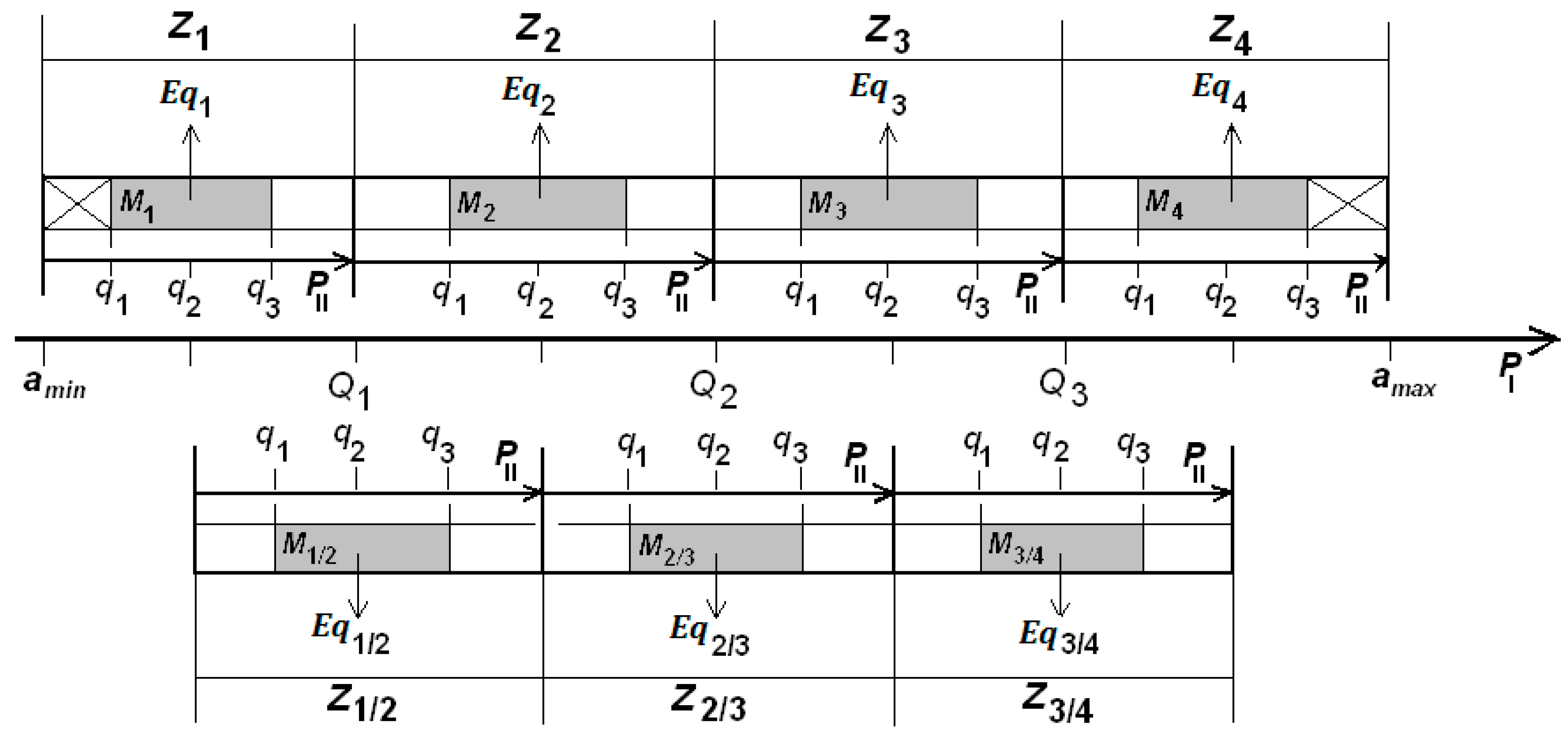
2.2.2. The Procedure of Soil Data Grouping

The method, schematically depicted in Figure 4, consists in giving a two-stage order of observations. At the first stage, the data collected (observations, cases) and consisting of the variables (dependent and independent), is divided into four main sets (Z₁, Z₂, Z₃, Z₄). Their limits are determined by: the minimum (a_min) and maximum (a_max) values, Q₁ (quartile 1), Q₂ (quartile 2–median) and Q₃ (quartile 3). They were calculated from the set of the numbers describing the order of observations, which was a consequence of the order (obtained by the appropriate ranking and weighting) determined according to the parameter selected for the arrangement (P_I). If more than one parameter was used at the same time, the rank of sums was used. Since the parameters selected to arrange at this stage showed similar correlation coefficients relative to the particles <0.02 mm, the regular type of rank with a weight of 1 was used.

At the second stage, the main sets were smoothed, consisting of the secondary ordering of the data in accordance with the parameters (P_II) other than at the first stage. When arranging the data, only one parameter was used at a time. After the second stage, the Z_x sets were divided into four sets (defined by quartiles). Because this operation concerned the subsets, they were marked with the lower case letters, i.e., q₁, q₂ and q₃.

Then, the multiple regression equations (Eq₁, Eq₂, Eq₃, Eq₄) were selected to predict the soil penetration resistance on the basis of the data contained between the q₁–q₃ quartiles, i.e., for the subsets M₁, M₂, M₃ and M_4. Such a procedure resulted in obtaining equations for soils with similar features. The data located between a_min and q₁, as well as q₃ and a_max, were rejected in the Z₁ and Z₄ sets. In the first case, these were the plastic soils close to the non-plastic soils; in the second case, these were soils with a very high content of fine particles, which are therefore uncommon.

To describe the dependence of the whole range of the variability of the soils researched, it was necessary to also include the omitted date. Thus, the equations Eq_1/2, Eq_2/3 and Eq_3/4 were also selected. These were obtained for the data from the quadrant interval of the supplementary sets Z_1/2, Z_2/3 and Z_3/4, marked on Figure 4 as M_1/2, M_2/3 and M_3/4, where Z_1/2, Z_2/3 and Z_3/4 were created after the first stage of ordering from the subsequent observations located on the data axis between the medians (q₂) of two neighbouring main sets, i.e., Z₁ and Z₂, Z₂ and Z₃ also Z₃ and Z₄.

3. Results and Discussion

3.1. Model Variables

Values of independent (w_w, ρ_d) and dependent (PR) variables of the regression model have been calculated for all cases within individual sites (

Table 2. Ranges of average values of physical properties determined for all cases within individual sites.

Site Designation	wpF2	ww	ρd	PR
	(% w/w)		(g·cm−3)	(kPa)
Cz	13.1–20.4	12.9–19.4	1.57–1.81	1387–2905 (217–1073/13.6–51.3)
De	15.3–23.6	8.8–22.8	1.44–1.65	976–4317 (172–1251/10.9–34.8)
Ku	11.3–22.4	10.1–18.5	1.57–1.73	1510–4220 (183–1492/9.6–39.1)
Sł	17.4–18.6	15.6–17.6	1.47–1.62	1274–1440 (338–658/23.5–51.7)
Lu	12.4–17.7	11.9–16.9	1.56–1.85	1260–3317 (234–1598/12.9–50.9)
No	14.9–22.7	15.5–21.7	1.51–1.79	837–2176 (136–821/7.3–39.9)
NP	19.7–26.3	15.8–22.4	1.32–1.65	853–2349 (194–637/17.3–41.7)
Ob1	22.1–31.3	19.1–29.1	1.32–1.56	213–2863 (96–661/6.0–39.5)
Ob2	12.7–18.8	8.7–19.4	1.41–1.71	313–4296 (73–986/11.0–43.9)
Os	12.5–22.7	11.7–21.5	1.56–1.80	1362–2768 (203–587/12.7–43.1)
Re	20.5– 9.6	14.3–24.9	1.32–1.57	1693–2449 (313–520/18.5–46.9)
Sk	14.1–43.8	14.2–42.4	1.27–1.80	849–2361 (98–649/11.5–35.4)
St	15.9–25.2	11.3–24.1	1.38–1.72	369–1999 (123–543/12.5–21)

Designations of places see Table 1; in the brackets are given: the standard deviation/the relative standard deviation.

). It can be seen that measurements of the PR were performed at moisture w_w close to that for matric potential pF 2. It can also be noticed that the range of PR values for cases within sites was characterized by high variability. The following values show the standard deviation or the relative standard deviation: the results of measurements of w_w, ρ_d and PR before grouping test. The relative standard deviation reached values around 50% of the measured PR.

3.2. Results of the Preliminary Grouping Tests

Table 3. Values of determination coefficient (R²) of multiple regression models for particular data sets (A–D4) obtained during preliminary grouping of observations in respect of content of particles <0.02 mm for dependence of penetration resistance (PR) on gravimetric moisture content and dry bulk density.

Values of the Multiple Regression Coefficient R2 for Particular Data Sets (A–D4)
A	B1	B2	C1	C2	C3	D1	D2	D3	D4
0.29	0.36	0.30	0.39	0.22	0.20	0.48	0.35	0.25	0.42

shows the values of the multiple regression coefficient (R²) for the dependence of the soil PR on the gravimetric moisture content and the dry bulk density obtained during the preliminary grouping tests (stacking) of the observations in respect of the particle content <0.02 mm, with their division for a different number of sets (A; B1–B2; C1–C3; D1–D4). The best effect was achieved by dividing the observations (cases) into four sets (D1–D4), in accordance with Figure 3. Dividing the observations into more sets than 4 caused a decrease of the R² value. This shows that the sets D1, D2, D3 and D4 (Table 3) are synonymous with those marked in Figure 4 as Z₁, Z₂, Z₃ and Z₄.

3.3. Selection of Parameters for Grouping

The presented method of the data grouping (Figure 4) required a limited number of grouping parameters used at both stages of possible combinations.

Table A2. Ranges of grouping parameters (the properties calculated on the basis of the results of the granulometric composition and the humus content) for individual sites in layer of 25–60 cm.

Site Designation	ρB	ρdB	nB	WPPb	Sz	ZD	SD	RCD	WPPz	S
	g∙cm−3	g∙cm−3	%	%	mm	m2∙100g−1	m2∙cm−3	g∙100g−1	%	–
Cz	2.45–2.53	1.39–1.50	41.5–44.7	17.5–27.0	0.011–0.033	60.0–125.0	158.9–331.0	0.76–2.28	20.1–30.1	0.69–2.79
De	2.41–2.54	1.34–1.50	41.2–46.4	19.4–28.0	0.007–0.039	35.4–162.2	93.7–429.8	0.41–2.13	19.7–36.5	0.58–3.27
Ku	2.44–2.58	1.38–1.57	39.6–45.0	13.9–29.8	0.008–0.070	32.5–140.2	86.3–371.5	0.72–4.22	13.0–27.3	0.38–2.94
Sł	2.53–2.55	1.49–1.52	40.7–41.4	17.6–19.82	0.034–0.046	39.9–48.9	105.9–129.5	0.58–0.81	19.0–22.2	1.84–3.04
Lu	2.49–2.54	1.45–1.51	41.2–42.9	18.0–23.0	0.020–0.037	53.2–95.6	141.0–253.3	0.60–2.30	20.2–26.2	0.59–3.35
No	2.47–2.52	1.41–1.49	41.6–43.9	20.0–25.8	0.014–0.032	47.7–111.1	126.3–294.5	0.92–3.36	18.84–26.1	0.41–2.09
NP	2.48–2.50	1.42–1.45	42.5–43.2	23.5–25.6	0.017–0.021	48.4–71.1	128.2–188.4	0.36–0.92	26.6–30.0	1.63–4.83
Ob1	2.37–2.44	1.27–1.37	44.9–47.8	29.4–36.1	0.004–0.010	83.9–187.7	222.5–497.5	0.46–1.49	31.6–40.8	0.84–5.71
Ob2	2.51–2.57	1.48–1.55	40.2–42.4	15.1–19.0	0.028–0.056	48.6–73.8	128.8–195.5	0.54–1.37	13.3–27.3	1.66–4.42
Os	2.49–2.55	1.44–1.52	40.7–43.1	16.5–23.6	0.018–0.045	44.8–103.5	118.8–274.3	0.74–2.08	17.6–24.8	0.79–2.58
Re	2.49–2.50	1.44–1.46	42.3–42.8	23.7–24.3	0.019–0.021	59.1–66.7	156.7–176.9	0.31–0.43	27.8–32.6	4.93–6.40
Sk	2.36–2.53	1.25–1.50	41.4–48.2	16.7–38.6	0.003–0.036	59.7–174.0	158.2–461.1	0.67–2.34	22.7–45.3	0.69–3.79
St	2.50–2.54	1.45–1.51	41.1–42.6	18.3–22.8	0.020–0.036	60.1–90.1	159.3–238.8	0.32–1.58	17.9–29.5	1.00–8.58

Caution: ρ_B—soil calculated density of solid particles; ρ_dB—calculated soil dry bulk density; n_B—soil total porosity; WPP_b—soil water capacity calculated without the participation of the organic matter; S_z—soil average grain diameter; Z_D—soil specific surface; S_D—soil dispersion index; RCD—soil readily–dispersible clay content; WPP_z—soil water capacity calculated with the participation of the organic matter; S—soil stability index.

in the Appendix A contains the calculated values of the grouping parameters. It was assumed that the parameters to be rejected would be less frequently used parameters that highly correlated with the other commonly used parameters and that were of a relatively low variability. P_I (stage I) parameters were used to rank (classify) the soils. When choosing P_I parameters, attention was paid to the fact that they were positively correlated with <0.02 mm and were calculated on the basis of information about the particle size distribution of soils. In the case of stage II (P_II), parameters were selected for smoothing Z_x sets. Therefore, they were calculated not only on the basis of information on the granulometric composition, but also on other selected soil characteristics, affecting the soil strength.

When selecting the parameters for the first stage of ordering (division of data into sets Z₁, Z_1/2, Z₂, Z_2/3, Z₃, Z_3/4, Z₄), special attention was paid to the results of the research conducted by Prusinkiewicz and Proszek [24], who consider that the external surface area, in spite of conventionality, is a good expression of the graining of the soil samples researched, reducing all grain size analysis results to only one characteristic value. However, taking into consideration the selection of parameters to smooth subsets Z_x (stage II—creating the subsets M₁, M_1/2, M₂, M_2/3, M₃, M_3/4, M₄), indicators related to the humus content in the soil were included because it is known that humus affects the soil strength [27,28]. The stability index (S) developed by Pieri [26] was also considered because the relation of humus content to the content of silt or clay fraction in soil is also important for the soil strength. The parameter determining the content of the readily-dispersible clay (RCD) related to the susceptibility of agricultural soils [25] to destruction was also considered. The Trzecki [23] equation taking into consideration the humus content was also tested to smooth the subsets when calculating the field water capacity (WPP_z).

Among the many parameters considered during preliminary work (stage I: ρ_B, ρ_dB, n_B, WPP_b, S_z, Z_D, S_D; stage II: RCD, S, WPP_z, P_L, L_L), a list of finally selected parameters used for soil grouping during the main works of stages I and II is presented in

Table 4. Parameters P of stages I and II finally adopted for grouping (see Figure 4).

Parameter
Stage I (sets: Z1, Z1/2, Z2, Z2/3, Z3, Z3/4, Z4)	Stage II (sets: M1, M1/2, M2, M2/3, M3, M3/4, M4)
1. Total porosity (nB)—in acc. with Brogowski [22] 2. Field water capacity—without the humus content taken into consideration (WPPb)—in acc. with Trzecki [23] 3. Specific surface (ZD), inverse of soil average grain diameter (1/Sz)—in acc. with Prusinkiewicz and Proszek [24]	1. Content of readily–dispersible clay (RCD)—in acc. with Czyż [25] 2. Stability index (S)—in acc. with Pieri [26] 3. Field water capacity—with humus content taken into consideration (WPPz)—in acc. with Trzecki [23]

. Because 1 to 3 parameters were used during the grouping in stage I, all had to be positively correlated to particles <0.02 mm. Therefore, the reverse value (1/S_z) was used for the average grain diameter.

When testing the different combinations of the adopted method of data grouping with the use of the parameters selected for grouping (Table 4), the goal was to find a variant for which the obtained multiple regression equation was characterized by the highest matching to the experimental data, where the adjustment was expressed by the value of the determination coefficient R² (

Table 5. Determination factor values (R²) for particular subsets (M_x) and selected “best” data grouping combinations obtained for dependency of penetration resistance (PR) on moisture gravimetric content and dry bulk density.

Combination Number	Grouping Parameter		The R2 Value of the Regression Equations Eqx Obtained for Individual Subsets of Mx Data
	Stage I	Stage II	M1	M1/2	M2	M2/3	M3	M3/4	M4
0	< 0.02 mm	-	0.53	0.56	0.07	0.24	0.48	0.40	0.40
1	ZD	-	0.56	0.50	0.32	0.33	0.34	0.41	0.50
2	nB	-	0.56	0.23	0.58	0.56	0.19	0.25	0.62
3	WPPb	-	0.50	0.25	0,61	0.40	0.49	0.35	0.40
4	1/Sz	-	0.54	0.21	0.49	0.55	0.01	0.33	0.63
5	1/Sz	RCD	0.55	0.50	0.68	0.47	0.27	0.29	0.55
6	ZD	WPPz	0.62	0.38	0.52	0.35	0.45	0.19	0.59
7	nB	WPPz	0.49	0.53	0.72	0.59	0.26	0.35	0.40
8	nB & 1/Sz	RCD	0.59	0.52	0.60	0.47	0.27	0.29	0.54
9 #	WPPb & ZD	WPPz	0.51	0.50	0.76	0.64	0.29	0.25	0.57
10	ZD & 1/Sz	WPPz	0.49	0.68	0.66	0.45	0.27	0.25	0.55
11	nB & WPPb & ZD	RCD	0.55	0.42	0.54	0.36	0.38	0.28	0.59
12	nB & WPPb & ZD	WPPz	0.48	0.46	0.80	0.60	0.27	0.26	0.56
13	nB & ZD & 1/Sz	RCD	0.54	0.36	0.53	0.34	0.30	0.27	0.61

Caution: ^# means the combination selected for further considerations; parameter markings, see Table 4.

). It can be seen that the R² values obtained for subsets M_x with respect to particle content <0.02 mm (combination 0) were on average higher than calculated for sets D1–D4 (Table 3). The use of other grouping parameters and the introduction of grouping stage P_II increased the value of R². However, increasing the number of parameters up to 3 of P_I stage no longer resulted in a significant increase in the R² value. Due to the determination coefficient, i.e., assuming maximum values in M_x subsets or close to them, for further considerations—selection of regression equations—the combination number 9 was chosen: P_I–WPP_b & Z_D, P_II–WPP_z.

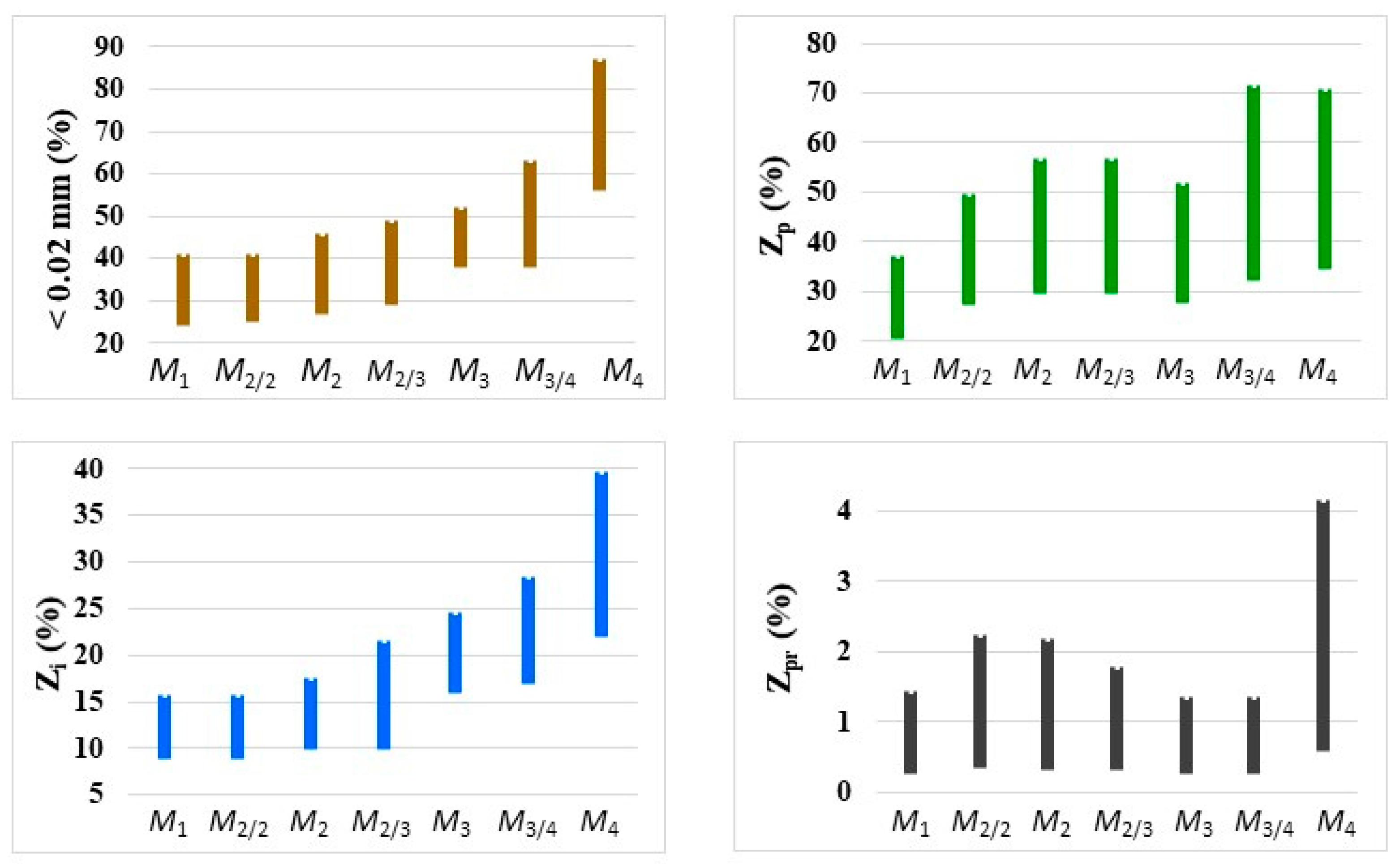
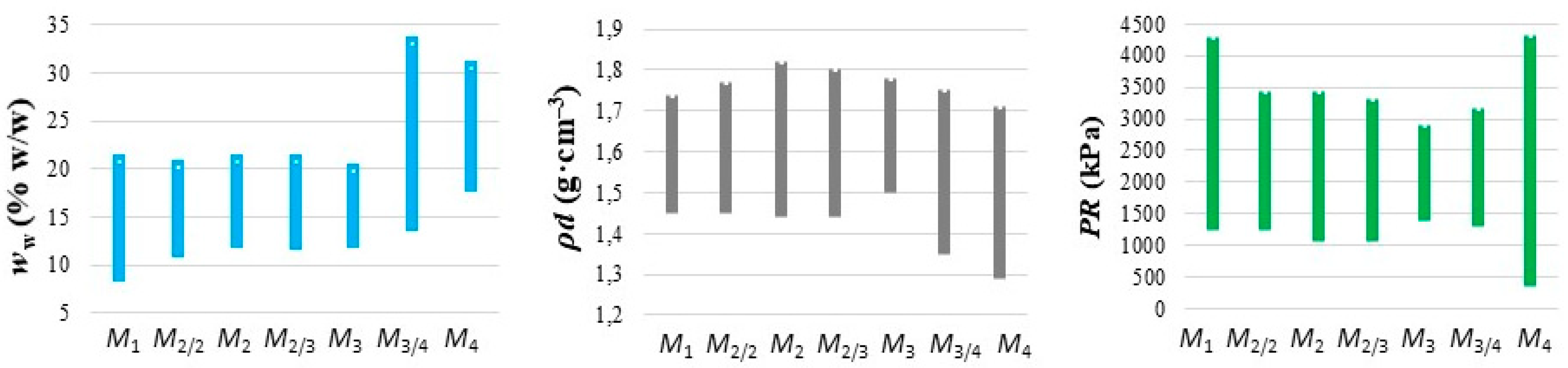
3.4. Characterization of Subsets after Data Grouping

Figure 5 presents the scopes of changes in the soil parameters selected for the particular data subsets (M_x), obtained after grouping the combination with the number 9. It can be seen that the particle content ranges <0.02, Z_p and Z_i are similar between subsets (M_x). With the largest range of values noted for subsets M_3/4 or M₄. The values of parameters of adjacent subsets overlap, which was intended and results from the proposed method of data grouping (Figure 4). The largest ranges of changes in parameter values presented in Figure 5 were noted in relation to the humus content (Z_pr). The maximum Z_pr values were on average 6 times higher than the minimum values. The wide range of changes in the Z_pr value in individual subsets of M_x indirectly justifies the second stage of data grouping (P_II).

After grouping the cases with the selected combination, soils with different granulometric groups were allocated to individual subsets (

Table 6. Soil texture for the particular data subsets (Mx), obtained after grouping with combination number 9 (see Table 5).

Soil Texture acc. USDA [29]
M1	M1/2	M2	M2/3	M3	M3/4	M4
SL(33), L(1)	L(19), SL(14) SiL(1)	L(24), SiL(6), SL(4)	L(28), SiL(5), SCL(1),	L(31), SCL(2), SiL(1)	L(20), CL(8), SiL(6)	SiL(12), CL(7), L(6), SiCL(5), SCL(2), SiC(2)

Designations: SL—sandy loam, SCL—sandy clay loam, L—loam, SiL—silt loam, CL—clay loam, SiC—silty loam, SiCL—silty clay loam; The number of cases included in a given granulometric group is given in brackets.

). This result indicates that the subsets obtained for the purpose of forecasting soil strength are not identical to a specific granulometric group. Nevertheless, the direction of changes is noticeable, i.e., from sandy loam soils to clayey soils.

Figure 6 shows the obtained values of the independent (w_w, ρ_d) and the dependent (PR) variables for individual subsets of data (M_x). The proposed method of data grouping caused a range of changes of independent variables in individual subsets of M_x. Significantly higher differentiation was obtained for subsets M_3/4 and M₄. For PR, larger value ranges occurred for subsets M₁ and M₄.

3.5. Regression Equations

Because of the high variability of the soil environment and, therefore, a large dispersion of the measurement results, the diverging observations (outliers) were searched prior to selecting the regression equations (Eq_x) for individual subsets (M_x). The observations exceeding the range of ± 2 standard deviations were excluded (

Table 7. Regression equations to calculate soil penetration resistance (PR) and their statistical evaluation.

Equation Number	Equation	F	p	R2	RMSE
Eq1	4452.7–169.7·ww–65.6·ρd NS	31.2	***	0.69	355.9
Eq1′	3809.9 –132.5·ww	23.7	***	0.46	323.5
Eq1/2	5607.1–167.6·ww–773.8·ρdNS	51.0	***	0.79	217.2
Eq1/2′	4077.5–147.8·ww	56.3	***	0.66	268.7
Eq2	3958.0–157.9·ww + 226.7·ρd NS	77.1	***	0.84	240.8
Eq2′	4325.5–158.1·ww	157.8	***	0.84	237.8
Eq2/3	3153.8 – 140.3·ww + 535.1·ρd NS	31.9	***	0.69	309.5
Eq2/3′	3931.4 – 133.5·ww	63.2	***	0.68	292.4
Eq3	1612.4 NS – 64.9·ww + 792.3·ρd NS	13.3	***	0.52	183.4
Eq3′	2929.5 – 66.4·ww	18.7	***	0.44	161.4
Eq3/4	4551.5–67.5·ww–873.4·ρd NS	10.5	***	0.48	293.7
Eq3/4′	2607.4–36.0·ww	13.8	***	0.35	325.5
Eq4	6098.0–160.5·ww–420.0·ρdNS	59.2	***	0.81	349.0
Eq4‘	5243.9–151.7·ww	92.7	***	0.76	385.1

F—Snedecor test, p—probability limit (***—p < 0.001), R²—determination coefficient, RMSE—the root mean square error, ^NS—non significant (significant at the p = 0.05 levels or less).

). The sign of the regression coefficients indicates the negative influence of the soil moisture on the value of its the penetration resistance. It can therefore be concluded that the derived equations map the tendency of soil strength changes as a function of soil moisture content in a proper manner, in accordance with the current state of knowledge.

The study confirmed that the current soil moisture is more useful for predicting the penetration resistance value than soil dry bulk density. The lack of a statistically significant impact of density (significant at the p = 0.05 levels or less) on the result of PR prediction was probably related to the fact that the research material was plastic soils with moisture similar to pF2 and a high content of clay particles (Table 2). This assumption is substantiated by the results of studies by Mosaddeghi et al. [7], who found that the soil dry bulk density may be of little use for forecasting soil strength as the content of clay in it increases. Table 7 shows the equations obtained for PR forecasting with (equations E_qx) and without (equations E_qx’) dry bulk density as a predictor.

Considering the variability of the soil environment derived within individual subsets of Mx, the regression equations E_qx (Table 7) are characterized by a relatively high rating. The calculated F, p, R² and RMSE assessment parameters have high or satisfactory values. All the dependencies received are statistically significant—p < 0.001 (the significance level = 0.05). However, matching the equations to the experimental data measured by the determination coefficient (R²) is satisfactory and only with the equation E_q3/4 is it less than 0.50. RMSE values for E_qx equations are close to the minimum standard deviations of the PR values measured in the field (see Table 2). Moreover, it shows that the variance inflation factor (VIF) calculated to check the degree of multicollinearity among predictors (the gravimetric moisture content and the dry bulk density) did not exceed the value of 1.6, which is indicative of multicollinearity among predictors [30].

In the case of E_qx’ equations (Table 7), it can be seen that the use of humidity only for PR prediction showed that matching the equations to the experimental data measured by the determination coefficient (R²) is also satisfactory and only with the equations E_q3′ and E_q3/4′ is it less than 0.50. The calculated RMSE for E_qx’ equations have values similar to those obtained for E_qx equations.

Due to the variety and number of factors that affect the PR measurement result [31], the equations for forecasting penetrometric resistance, obtained by other authors, are difficult to compare with the results of this work. Nevertheless, it is possible to compare the parameters of the statistical evaluation of equations obtained for the same predictors. The R² and RMSE values given in

Table 8. Affiliation criteria for particular series of Eq_x’ equations (Table 7) for cases from the verification set—median values of selected soil parameters for particular subsets (M_x) of basic set.

Parameter	Values of Soil Parameters for Particular Subsets (Mx)
	Column Number—Equation Number
	1–Eq1	2–Eq1/2	3–Eq2	4–Eq2/3	5–Eq3	6–Eq3/4	7–Eq4
<0.02	24.0–31.5	31.6–33.5	33.6–39.5	39.6–46.5	46.6–52.5	52.6–61.5	61.6–87.0
Zp	20.6–31.0	31.1–33.0	33.1–34.5	34.6–35.5	35.6–36.5	36.6–41.5	41.6–70.6
Zi	8.8–12.2	12.3–13.6	13.7–15.9	16.0–18.9	19.0–22.7	22.8–25.9	26.0–39.7
PL	13.0–15.9	16.0–17.1	17.2–17.9	18.0–18.9	19.0–20.6	20.7–24.7	24.8–32.3
LL	14.8–23.2	23.3–24.6	24.7–26.9	27.0–30.9	31.0–37.7	37.8–45.3	45.4–67.0
ZD	43.5–59.9	60.0–64.7	64.8–75.7	75.8–90.1	90.2–106.2	106.3–122.1	122.2–170.6
Sz	0.035–0.049	0.028–0.034	0.025–0.027	0.022–0.024	0.017–0.021	0.013–0.016	0.003–0.012
WPPb	15.1–19.2	19.3–20.7	20.8–21.4	21.5–22.5	22.6–25.2	25.3–29.9	30.0–38.6

For remaining markings–see section “Materials and Methods”.

are similar to the results obtained by other authors [12,13] using moisture content (w_w) as a predictor of the PR.

Considering the assessment of the results presented in Table 7 and the need for simplifying the procedure, further considerations were made only in relation to the equations E_qx’.

The regression equations (Table 7) were assessed with the use of the cases included in the validation set. The choice of equations (E_qx’) for individual cases of the verification set was made using the criteria (soil parameters), which determine the average values calculated from the medians of two adjacent subsets (M_x) and the extreme values for the subsets M₁ and M₄ (see Table 8). The choice of equations was made in two ways. First, attention was paid to which column contains the values of soil parameters from the validation set. When more than half of the criteria used pointed to a specific column, the choice of the equation was considered complete. In the case where there was no clear indication of the column (equation), the second method was used. Each result of comparing the parameters from the validation set with the affiliation criteria was assigned a number equal to the column number (equation). In this way, a table (matrix) of results was created with numbers that could have values from 1 to 7. The sum of all numbers of the matrix divided by the number of criteria used (parameters compared), and then rounded to whole numbers, indicated the number of the equation.

In an attempt to simplify the selection of regression equations to predict PR values (Table 7), various combinations of criteria (parameters) listed in Table 8 were tested.

The obtained values of the relative prediction errors (δ_p) of the soil PR were also analyzed (

Table 9. Values of mean relative error of the prognosis (δ_p) for particular equations E_qx’ (Table 7) using selected combinations of criteria listed in Table 8 and data contained in the validation set.

Parameter Used (Table 8)	Values of Mean Relative Error of the Prognosis (%)
	Eq1′	Eq1/2′	Eq2′	Eq2/3′	Eq3′	Eq3/4′	Eq4′
ZD	15(9.9)	14(8.1)	17(10.2)	15(8.4)	17(10.4)	19(10.9)	17(11.0)
PL, WPPb, ZD	17(8.9)	14(10.8)	16(5.1)	13(8.5)	17(9.6)	18(10.4)	18(9.2)
<0.02, PL, ZD, Sz, WPPb	17(8.0)	13(9.8)	13(4.3)	11(8.9)	15(10.1)	18(10.7)	19(8.7)
<0.02, Zp, Zi, PL, LL, ZD, Sz	16(10.2)	13(9.7)	17(8.2)	16(10.2)	17(7.6)	19(8.9)	19(8.8)

For remaining markings—see section “Materials and Methods”; the standard deviation is given in the brackets.

). The δ_p error is the difference between the values measured and predicted divided by the values measured. It may be noted that the mean values δ_p are smaller than 20%. It can be seen, taking into account the variability of the property that is PR (Table 2), that for the selection of the regression equation for the cases contained in the validation set it was sufficient to use information about Z_D. Although, on average, better results were obtained using 3 or 5 criteria, the obtained values of the forecast error and its standard deviation were at a similar level. The use of up to 7 parameters to choose the equation did not significantly improve the quality of the PR prediction.

The presented method of data grouping allowed us to obtain a series of 7 equations for predicting the PR of plastic soils. Applying the selected equation requires only one predictor (the gravimetric moisture content). To choose the equation, it is sufficient to provide information about one parameter characterizing the soil surface (the specific surface). It should be added that in the literature you can find examples of equations that require the use of more predictors [8,32,33].

3.6. Methodological Limitations

The grouping method presented in the paper as well as the obtained regression equations for forecasting soil penetrometric resistance are characterized by certain limitations.

Using the proposed method requires collecting a large set of output data. Most authors recommend that one should have at least 10 to 20 times as many observations (cases, respondents) as one has variables [34].

Verification of the proposed method, from the point of view of assessing the values of grouping parameters and variables of the regression model, may be difficult due to the measurement methods used in this work and the conditions for making measurements. The soil bulk density determination was performed using the core sampling method (volumetric cylinder method), which is the most common method used to determine bulk density agricultural soils [35]. Researchers use cylinders of different sizes, which may be affected by the result of the soil properties determined [36,37,38]. The Bouyoucos Casagrande method modified by Prószyński was used to measure the particle size distribution of soil, which is one of the methods commonly used, although automated methods are currently gaining increasing popularity [39].

The humus content was determined with the use of the Tiurin method. This method allows you to calculate the humus content based on the determined amount of organic carbon. The Tiurin method is therefore not a modern method that allows advanced analysis of soil organic matter composition [40,41,42]. Determining the humus content with the use of the Tiurin method was, however, sufficient to calculate the values of such grouping parameters as: RCD, S and WPPz (Table 4). It should be added here that, in the light of recent research, organic matter persistence in soil is seen as a property of the ecosystem [43], which means that the results of this study should be treated rather for local application. It should be emphasized, however, that the parameters used to compile the data are not a closed list (see Section 3.3). Verification of the proposed DGM can be undertaken by using data (cases) for other, available or determinable parameters of selected soils. At the same time, other measuring methods can be used to determine soil properties such as humus content or granulometric composition.

The use of regression equations obtained in this work for PR forecasting also has limitations. First, the equations were obtained for the subsoil of plastic soils with a similar original, i.e., glacial deposit. Secondly, the choice of equations is made using the affiliation criteria for a particular series of Eqx ‘equations (Table 8), which are determined, with the exception of P_L and L_L, on the basis of soil granulometric composition. The use of a method other than the Bouyoucos Casagrande method modified by Prószyński may result in obtaining values of affiliation criteria that will cause the selection of the wrong equation for PR forecasting.

4. Conclusions

A new data grouping method (DGM) was developed for predicting the penetration resistance of plastic soils. The method is based on the division of the results of measurements into groups with narrow ranges of soil grain variability, taking into account humus content.

The study showed that it is possible to forecast the soil penetration resistance on the basis of two independent variables: gravimetric moisture content and bulk density. Statistical evaluation indicates that the dry bulk density is much less useful for predicting the penetration resistance of plastic soils than soil moisture. The study also showed that it is possible to forecast the soil penetration resistance on the basis of the gravimetric moisture content and the specific surface. Verification of the obtained regression equations showed that the mean relative errors of the prognosis of penetration resistance were less than 20%.

The method is universal, because it is independent of existing soil grain classifications. On the other hand, the DGM method may have some limitations. The method has been verified so far for plastic soils. Moreover, selection of equations for PR forecasting may be sensitive to equations used for soil granulometric composition determination.

Further research will focus on application of the DGM method in relation to other soil properties, for example vane shear stress and the pre-compression stress.

References

1. Van den Akker, J.J.H.; Arvidsson, J.; Horn, R. Introduction to the special issue on experiences with the impact and prevention of subsoil compaction in the European Union. Soil Till. Res. 2003, 73, 1–8. [Google Scholar] [CrossRef]
2. Hadas, A.; Shmulevich, O.; Hadas, O.; Wolf, D. Forage wheat yields as affected by compaction and convention vs. wide frame tractor traffic patterns. Trans. ASAE 1990, 33, 79–85. [Google Scholar] [CrossRef]
3. Oskoui, K.E.; Voorheers, W.B. Economical consequences of soil compaction. Trans. ASAE 1991, 34, 2317–2323. [Google Scholar] [CrossRef]
4. Alakukku, L. Persistence of soil compaction due to high loads traffic. II Long-term effect on the properties of fine–textured and organic soils. Soil Till. Res 1996, 37, 223–238. [Google Scholar] [CrossRef]
5. Krasowicz, S.; Oleszek, W.; Horabik, J.; Dębicki, R.; Jankowiak, J.; Stuczyński, T.; Jadczyszyn, J. Rational management of the soil environment in Poland. Pol. J. Agron 2011, 7, 43–58. (In Polish) [Google Scholar]
6. Olesen, J.E.; Munkholm, L.J. Subsoil loosening in a crop rotation for organic farming eliminated plough pan with mixed effects on crop yield. Soil Till. Res. 2007, 94, 376–385. [Google Scholar] [CrossRef]
7. Mosaddeghi, M.R.; Hemmat, A.; Hajabbasi, M.A.; Alexandrou, A. Pre-compression stress and its relation with the physical and mechanical properties of a structurally unstable soil in central Iran. Soil Till. Res. 2003, 70, 53–64. [Google Scholar] [CrossRef]
8. Dexter, A.R.; Czyż, E.A.; Gate, O.P. A method for prediction of soil penetration resistance. Soil Till. Res. 2007, 93, 412–419. [Google Scholar] [CrossRef]
9. Arvidsson, J.; Keller, T. Comparing penetrometer and shear vane measurements with measured and predicted mouldboard plough draught in a range of Swedish soils. Soil Till. Res. 2011, 111, 219–223. [Google Scholar] [CrossRef]
10. Motavalli, P.P.; Anderson, S.H.; Pengthamkeerati, P.; Gantzer, C.J. Use of soil cone penetrometers to detect the effects of compaction and organic amendments in claypan soils. Soil Till. Res. 2003, 74, 103–114. [Google Scholar] [CrossRef]
11. Horn, R.; Fleige, H. A method for assesing the impact of load on mechanical stability and on physical properties of soils. Soil Till. Res. 2003, 73, 89–99. [Google Scholar] [CrossRef]
12. Busscher, W.J.; Bauer, P.J.; Camp, C.R.; Sojka, R.E. Correction of cone index for soil water content differences in a coastal plain soil. Soil Till. Res. 1997, 43, 205–217. [Google Scholar] [CrossRef]
13. Vaz, C.M.P.; Manieri, J.M.; de Maria, I.C.; Tuller, M. Modeling and correction of soil penetration resistance for varying soil water content. Geoderma 2011, 166, 92–101. [Google Scholar] [CrossRef]
14. Vaz, C.M.P.; Manieri, J.M.; de Maria, I.C.; Tuller, M.; van Genuchten, M.T. Scaling the Dependency of Soil Penetration Resistance on Water Content and Bulk Density of Different Soils. Soil Sci. Soc. Am. J. 2013, 77, 1488–1495. [Google Scholar] [CrossRef] [Green Version]
15. Lebert, M.; Horn, R. A method to predict the mechanical strenght of agricultural soils. Soil Till. Res. 1991, 19, 275–286. [Google Scholar] [CrossRef]
16. Fritton, D.D. Evaluation of pedotransfer and measurement approaches to avoid soil compaction. Soil Till. Res. 2008, 99, 268–278. [Google Scholar] [CrossRef]
17. Finke, R.; Hartwich, R.; Dudal, R.; Ibanez, J.; Jamagne, M.; King, D.; Montanarella, L.; Yassoglou, N. Georeferenced Soil Database for Europe. Manual of Procedures. Version 1.1 by European Soil Bureu Scientific Committee; EUR 18092 EN ©European Communities, Office for Official Publications of the European Communities: Luxembourg, 2001. [Google Scholar]
18. Lipiński, J. Quantified system of description of the soil’s graining. Wiadomości Instytutu Melioracji i Użytków Zielonych 1996, 19, 91–100. (In Polish) [Google Scholar]
19. Constantini, A. Relationships between cone penetration resistance, bulk density, and moisture content in uncultivated, repacted, and cultivated hardsetting and non-hardsetting soils from the coastal lowlands of South-East Queensland. N. Zealand J. For. Sci. 1996, 26, 395–412. [Google Scholar]
20. Alakukku, L. Experience with soil compaction. In Experiences with the impact and prevention of subsoil compaction in the European Community. In Proceedings of the Concerted Action “Experiences with the impact of subsoil compaction on soil, crop and environment and ways to prevent subsoil compaction”, Wageningen, The Netherlands, 28–30 May 1998. [Google Scholar]
21. ISO. Soil Quality–Determination of the Potential Cation Exchange Capacity and Exchangeable Cations Using Barium Chloride Solution Buffered at pH. ISO 13536. 1995. [Google Scholar]
22. Brogowski, Z. An attempt of calculation of same physical properties of soils on the basis of granulometric analysis. Roczniki Gleboznawcze 1990, 41, 17–28. (In Polish) [Google Scholar]
23. Trzecki, S. Determination of water capacity of soils on the basis of their mechanical composition. Rocz. Gleboz. (suppl.) 1974, 25, 33–44. [Google Scholar]
24. Prusinkiewicz, Z.; Proszek, P. “Texture”–the program of computer interpretation of results of soil particle size analysis. Rocz. Glebozn. 1990, 41, 5–16. (In Polish) [Google Scholar]
25. Czyż, E.A. Quantitative and spatial characteristic of polish agricultural soils to destruction. Inżynieria Rol. 2005, 3, 15–22. (In Polish) [Google Scholar]
26. Schroth, G. Measuring the Role of Soil Organic Matter in Aggregate Stability. In Trees, Crops and Soil Fertility Concepts and Research Methods; Schroth, G., Sinclair, F.L., Eds.; CABI Publishing: Wallingford, UK, 2003; pp. 204–207. ISBN 0-85199-593-4. [Google Scholar]
27. Dexter, A.R.; Richard, G.; Arrouays, D.; Czyż, E.A.; Jolivet, E.A.; Duval, O. Complexed organic matter controls soil physical properties. Geoderma 2008, 144, 620–627. [Google Scholar] [CrossRef]
28. Soane, B.D. The Role of Organic Matter in Soil Compactibility: A Review of Some Practical Aspects. Soil Till. Res. 1990, 16, 179–201. [Google Scholar] [CrossRef]
29. Particle size distribution and textural classes of soils and mineral materials—classification of Polish Society of Soil Science 2008. Rocz. Glebozn. Soil Sci. Annu. 2009, 60, 5–16. (In Polish)
30. Kutner, M.H.; Nachtsheim, C.; Neter, J.; Li, W. Applied Linear Statistical Models; McGraw-Hill/Irwin: New York, NY, USA, 2005; ISBN 0-07-238688-6. [Google Scholar]
31. Pukos, A.; Walczak, R. Methodical aspects of the constuction of soil penetrometers as applied to the evaluation of soil compaction. Zesz. Probl. Postępów Nauk Rol. 1990, 308, 149–159. [Google Scholar]
32. Elaoud, A.; Hassen, H.B.; Salah, N.B.; Masmoudi, A.; Chehaibi, S. Modeling of soil penetration resistance using multiple linear regression (MLR). Arab. J. Geosci. 2017, 10, 442. [Google Scholar] [CrossRef]
33. Gao, W.; Whalley, W.R.; Tian, Z.; Liu, J.; Ren, T. A simple model to predict soil penetrometer resistance as a function of density, drying and depth in the field. Soil Till. Res. 2016, 155, 190–198. [Google Scholar] [CrossRef]
34. TIBCO Software Inc. Statistica (Data Analysis Software System), Version 13. 2017; (Available in: Statistica Help, Statistica Electronic Manual).
35. Casanova, M.; Tapia, E.; Seguel, O.; Salazar, O. Direct measurement and prediction of bulk density on alluvial soils of central Chile. Chil. J. Agric. Res. 2016, 76, 105–113. [Google Scholar] [CrossRef] [Green Version]
36. Al-Shammary, A.A.G.; Kouzani, A.Z.; Kaynak, A.; Khoo, S.Y.; Norton, M.; Gates, W. Soil bulk density estimation methods: A review. Pedosphere 2018, 28, 581–596. [Google Scholar] [CrossRef]
37. Piccoli, I.; Schjønning, P.; Lamandé, M.; Zanini, F.; Morari, F. Coupling gas transport measurements and X-ray tomography scans for multiscale analysis in silty soils. Geoderma 2019, 338, 576–584. [Google Scholar] [CrossRef]
38. Lucas, M.; Vetterlein, D.; Vogel, H.J.; Schlüter, S. Revealing pore connectivity across scales and resolutions with X-ray CT. Eur. J. Soil Sci. 2020. [Google Scholar] [CrossRef] [Green Version]
39. Warzyński, H.; Sosnowska, A.; Harasimiuk, A. Effect of variable content of organic matter and carbonates on results of determination of granulometric composition by means of Casagrande’s areometric method in modification by Prószyński. Soil Sci. Annu. 2018, 69, 39–48. [Google Scholar] [CrossRef]
40. Sutton, R.; Sposito, G. Molecular structure in soil humic substances: The new view. Environ. Sci. Technol. 2005, 39, 9009–9015. [Google Scholar] [CrossRef]
41. Lehmann, J.; Solomon, D.; Kinyangi, J.; Dathe, L.; Wirick, S.; Jacobsen, C. Spatial complexity of soil organic matter forms at nanometre scales. Nat. Geosci. 2008, 1, 238–242. [Google Scholar] [CrossRef]
42. Kleber, M.; Johnson, M.G. Advances in understanding the molecular structure of soil organic matter: Implications for interactions in the environment. Adv. Agron. 2010, 106, 77–142. [Google Scholar]
43. Schmidt, M.W.I.; Torn, M.S.; Abiven, S.; Dittmar, T.; Guggenberger, G.; Janssens, I.A.; Kleber, M.; Kögel-Knabner, I.; Lehmann, J.; Manning, D.A.C.; et al. Persistence of soil organic matter as an ecosystem property. Nature 2011, 478, 49–56. [Google Scholar] [CrossRef] [Green Version]
Figure 1. A schematic of the methodology of the presented study.
Agronomy 10 00578 g001
Figure 2. Scheme of creating data cases for each measurement term of the soil layer in each soil pit—an example for a 25–30 cm layer.
Agronomy 10 00578 g002
Figure 3. The method of division of soils into a different number of sets (A; B1–B2; C1–C3; D1–D4) during preliminary research.
Agronomy 10 00578 g003
Figure 4. Method of division of soils into sets (Z1, Z1/2, Z2, Z2/3, Z3, Z3/4, Z4) and subsets (M1, M1/2, M2, M2/3, M3, M3/4, M4) used to create regression equations (Eq1, Eq1/2, Eq2, Eq2/3, Eq3, Eq3/4, Eq4) to the soil penetration resistance (PR) in relation to ordering parameters PI (stage I) and PII (stage II).
Agronomy 10 00578 g004
Figure 5. Ranges of selected soil parameter values for the particular data subsets (Mx), obtained after grouping with combination number 9 (see Table 5): Designations: <0.02, Zp and Zi–soil particle fraction content, respectively: <0.02 mm, 0.05–0.002 mm and <0.002 mm, Zpr–soil humus content.
Agronomy 10 00578 g005
Figure 6. The ranges of changes in the values of the independent (ww, ρd) and the dependent (PR) variables for individual subsets of data (Mx), obtained after soil grouping with combination number 9 (see also Table 5).
Agronomy 10 00578 g006