Article

Digital Count of Corn Plants Using Images Taken by Unmanned Aerial Vehicles and Cross Correlation of Templates

by
Héctor García-Martínez
1,
Héctor Flores-Magdaleno
1,*,
Abdul Khalil-Gardezi
1,
Roberto Ascencio-Hernández
1,
Leonardo Tijerina-Chávez
1,
Mario A. Vázquez-Peña
2 and
Oscar R. Mancilla-Villa
3
1
Colegio de Postgraduados, Carretera México-Texcoco Km. 36.5, Montecillo, Texcoco 56230, Mexico
2
Departamento de Irrigación, Universidad Autónoma Chapingo, Carretera México-Texcoco, km 38.5, Chapingo 56230, Mexico
3
Centro Universitario de la Costa Sur, Universidad de Guadalajara, Avenida Independencia Nacional 151, Autlán 48900, Mexico
*
Author to whom correspondence should be addressed.
Agronomy 2020, 10(4), 469; https://doi.org/10.3390/agronomy10040469
Submission received: 17 February 2020 / Revised: 18 March 2020 / Accepted: 26 March 2020 / Published: 28 March 2020
(This article belongs to the Section Innovative Cropping Systems)

Abstract

:
The number of plants, or planting density, is a key factor in corn crop yield. The objective of the present research work was to count corn plants using images obtained by sensors mounted on an unmanned aerial vehicle (UAV). An experiment was set up with five levels of nitrogen fertilization (140, 200, 260, 320 and 380 kg/ha) and four replicates, resulting in 20 experimental plots. The images were taken at 23, 44 and 65 days after sowing (DAS) at a flight altitude of 30 m, using two drones equipped with RGB sensors of 12, 16 and 20 megapixels (Canon PowerShot S100_5.2, Sequoia_4.9, DJI FC6310_8.8). Counting was done through normalized cross-correlation (NCC) for four, eight and twelve plant samples or templates in the a* channel of the CIELAB color space because it represented the green color that allowed plant segmentation. A mean precision of 99% was obtained for a pixel size of 0.49 cm, with a mean error of 2.2% and a determination coefficient of 0.90 at 44 DAS. Precision values above 91% were obtained at 23 and 44 DAS, with a mean error between plants counted digitally and visually of ±5.4%. Increasing the number of samples or templates in the correlation estimation improved the counting precision. Good precision was achieved in the first growth stages of the crop when the plants do not overlap and there are no weeds. Using sensors and unmanned aerial vehicles, it is possible to determine the emergence of seedlings in the field and more precisely evaluate planting density, having more accurate information for better management of corn fields.

1. Introduction

Corn, together with wheat and rice, is one of the most important cereals in the world; it supplies nutritional elements to human beings and animals, being a basic raw material of the transformation industry to produce starch, oil, proteins, alcoholic drinks, food sweeteners and fuel [1]. Planting density (number of plants per unit area), the number of cobs per unit area, the number of kernels per cob and kernel weight are the grain yield components that have an impact on the reachable yield of corn [2]. Several studies have analyzed the response of corn yield to planting density [3,4], concluding that planting density is a key component in corn yield. The determination of planting density or the number of plants per hectare is important information to evaluate the physiological characteristics of the crop, and ultimately, the final yield. Yield can be better estimated by including the precise number of plants in the models, also to identify the optimum planting density to manage production in corn growing.
With the development of technology, new aerial platforms have become available to acquire images using mounted sensors with high spatial and temporal resolution to detect and quantify crop variations; such is the case of unmanned aerial vehicles (UAV) [5,6,7]. At least four pixels are necessary to detect the smallest objects on an image [8]. Camera focal length and flight height define the image scale [9], It is of great importance to define the optimal pixel size according to the specific objectives and the crop characteristics [10]. Image resolution and object size are critical parameters in the accurate classification of vegetation [11], thus the sensor type used in image capture plays an important role in monitoring the vegetation. UAVs are flexible in the timing of image acquisition, without being limited by weather or terrain conditions, and are equipped with a range of RGB, multispectral, hyperspectral, thermal and LIDAR sensors [12]. RGB sensors capture radiation in the visible electromagnetic spectrum of red, green and blue bands, while common multispectral sensors are widely used due to obtaining spectral information in the red band, the near-infrared and red edge for monitoring vegetation, on the other hand, hyperspectral sensors capture reflectance in several narrow spectral bands (5–10 nm) [13,14]. Commercial RGB cameras are less expensive than multispectral or hyperspectral sensors and have high spatial resolution.
The images captured by these cameras are used to calculate vegetation indexes (IV) and to generate digital elevation models and plant height maps [15]. This technology has been successfully implemented to estimate biomass, estimate the fractional plant cover, height and weed detection and classification, [16,17,18,19,20]. Recently, RGB images obtained with these platforms have been used to count plants in safflower, wheat, rapeseed and germination in cotton and potato [12,21,22,23,24,25]. UAV platforms offer advantages to estimate corn plant counting and planting density. Some methods used in automatic counting of plants are affected by the growth stages of the crop, with different estimations for different growth stages [23,26]. Also, the presence of weeds and blurry effects in the images affects automatic corn plant counting, causing errors [22]. Zhang et al. [27] Extracted corn plants using vegetation indices and image segmentation techniques, on the other hand, Shuai et al. [28] applied the same method for counting corn plants and found accuracies greater than 95%. Gnädinger y Schmidhalter [22] counted corn plants in images, improving the image contrast and using segmentation techniques with an error smaller than 5%; some other authors used deep learning, segmentation algorithms and neural networks to count corn plants. [29,30,31].
The use of conventional RGB (Red, Green, Blue) digital images tends to be a low-cost alternative [32]. Some studies have been done to identify and separate the vegetation in crop images [33,34] using vegetation indexes (excess green index, ExG; vegetative index, VEG, others). Other studies have used conversions from the RGB color model to HSI, CIELAB and CIELUV color models, extensively, and successfully in order to separate the green color (vegetation) from the images and provide phenotypic and genotypic data at different growth conditions [35,36,37,38]. The CIELAB color model depends less on illumination [39] defining colors more according to the color perception by the human eye. This color model is considered uniform, this is to say, the distance between two colors is a linear color space that corresponds to the differences perceived between them [40]. The CIELAB color space is based on the concept that colors can be considered as combinations of red and yellow; red and blue; green and yellow; and green and blue. To determine the exact combination of colors of a product, coordinates are assigned in a three-dimensional color space (L*, a*, b*). The three color coordinates are luminosity, red/green coordinates and yellow/blue coordinates, respectively [41].
Object detection methods, like template comparison, are used in remote sensing to discriminate objects present in an image and their location [42]. Template comparison is one of the first and simplest methods but involves a high error margin in complex images [43,44]. In template comparison, understood as a technique to classify objects, a template or image sample is used and the general image is scanned to find the sample image through normalized cross-correlation. Correlation is a measure of the degree at which two variables or signals agree, not necessarily in real values but rather in the general performance of the same variables or signals; in the case of images, these two variables being the corresponding pixel values in both images (Pattern and image) [45]. Koh et al. [12] used the template comparison method to detect safflower seedlings in the early stages of growth, using a group of templates obtaining an R squared of 0.86 between manual and digital counts. Nuijten et al. [44] used this method to classify crops with a precision of 99.8%, Kalantar et al. [46] employed template comparisons in the oil palm count finding precisions around 86%.
As far as we know the normalized cross-correlation and template comparison, in combination with the CIELAB color space has not been reported in the literature for the corn plant count, therefore, this paper investigates whether this relatively simple methodology can be accurate in corn plant counting. A corn crop was established to obtain images using an unmanned aerial vehicle platform with RGB sensors, obtaining images at different stages of crop development to evaluate automatic counting precision through the use of templates and normalized cross-correlation (NCC), as well as observe the differences in precision using three types of RGB Sensors.

2. Materials and Methods
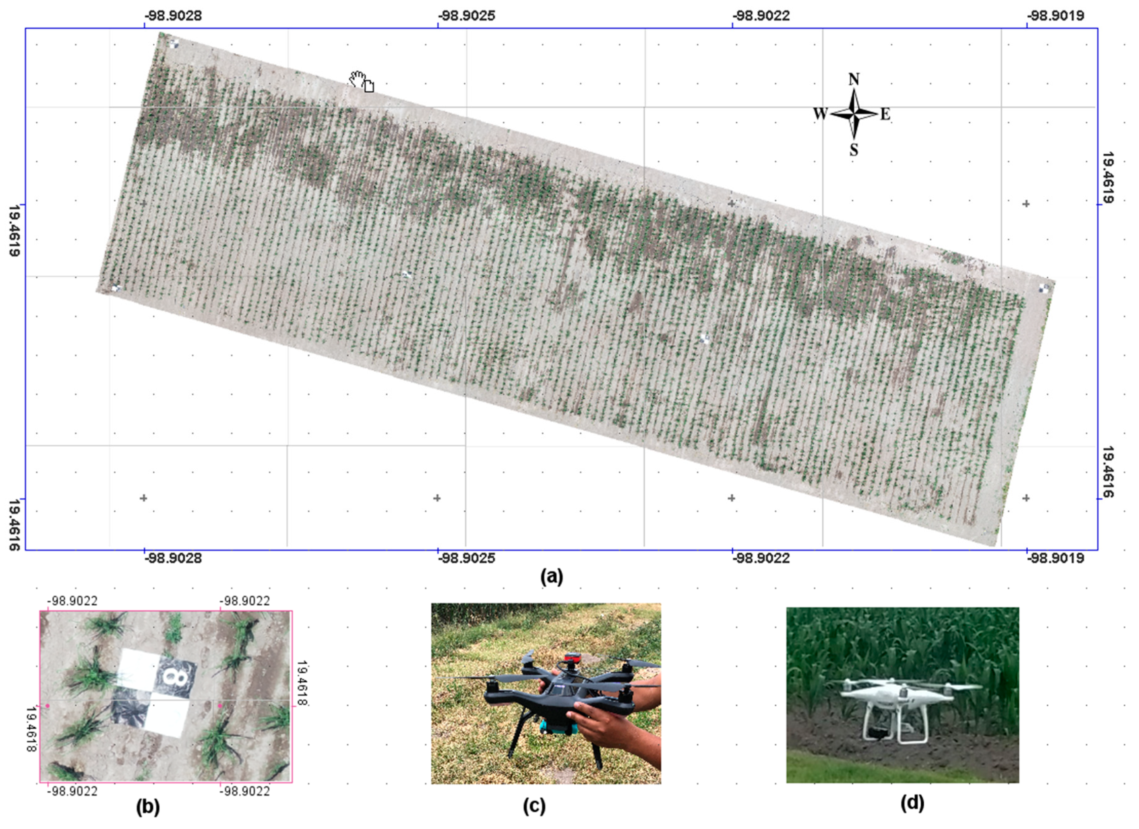
2.1. Study Site

The experiment was established on April 5th, 2018 in an experimental plot in the Colegio de Postgraduados, Campus Montecillo, located on the Mexico-Texcoco highway, km 36.5, Montecillo, Texcoco (19°27′40.58″ N, 98°54′8.57″ W, 2250 MASL). Soil texture is sandy loam with an apparent density of 1.45 g cm−3, O.M. 1.59%, pH 9.1 and electrical conductivity of 1.72 dS m−1. Five nitrogen levels were evaluated (140, 200, 260, 320 and 380 kg ha−1) in a completely randomized block design with four replicates, resulting in 20 experimental units (120 m2 per unit) of the Asgrow Albatross corn variety. A drip irrigation system was designed using drip tape and drippers separated to 20 cm and 1.6 Lh−1 water use in each experimental unit. The five nitrogen levels were applied directly with the irrigation water at 30% dose during the first 40 days, 50% dose from 40 to 80 days and 20% dose after 80 days. Sowing was done manually, with 80 cm between rows, and 30 cm between plants with three seeds; weeds were controlled by hand.

2.2. Image Acquisition and Processing

Aerial images were taken with an unmanned aerial vehicle at a height of 30 m over the terrain, covering a crop area of 2500 m2, at 27, 44 and 67 days after sowing (DAS) during 2018. Table 1 shows the summary of the flights.
A 3DR SOLO drone (3D Robotics, Berkeley, CA, USA) was used, 20 min flight autonomy, with a precision range of 1–2 m where a sensor is placed for image acquisition. To capture the images, the drone was equipped with a Canon S100 camera (Canon, Tokyo, Japan), weighing 200 g, high sensitivity CMOS sensor by Canon, type 1/17, 12.1 megapixels, real color with three channels (red, green, blue—RGB), image size 4000 × 3000 pixels in each channel. Another type of sensor used was a multispectral Parrot Sequoia (Parrot SA, Paris, France), weighing 72 g, to capture RGB images at 16 megapixels, image size 4608 × 3456 pixels. It also incorporates 4 sensors in green (550 nm), red (660 nm), red edge (725 nm) and near infrared (790 nm) channels, 1.2 megapixels, image size 1280 × 960 pixels and a 35 g solar sensor. Flights were carried out a height of 30 m and 80% frontal and lateral overlap during crop development from April 27th to July 19th, 2018, between 12:00 p.m. and 3:30 p.m. A UAV flight was carried out at 44 DAS with a Dji Phantom 4 drone (DJI, Shenzhen, Guangdong, China) equipped with a 1-inch CMOS sensor, 20 megapixels in compound true color with three channels (red, green, blue—RGB), image size 5472 × 3078 pixels in each channel; load-capacity of 1.388 kg and 30 min flight autonomy. It is equipped with a GPS/GLONASS satellite positioning system with a vertical precision range of ±0.5 m and a horizontal precision range of 1.5 m.
Flight configuration to take the images was done using the Pix4D capture application for mobile phones. Six ground control points (GCP) were placed. Figure 1 shows the distribution of the GCPs. For each flight, a Hi-target GNSS RTK V90 PLUS system (Hi-Target Surveying Instrument Co., Ltd, Guangzhou, China) was used to register the center of each control point with RTK precision, H: 8 mm + 1 ppm RMS and V: 15 mm + 1 ppm RMS. The images captured by the different sensors and the ground control points were processed with the Pix4D mapper software (Pix4D SA, Lausanne, Switzerland) for each flight, obtaining an orthomosaic, a surface digital model and a point cloud.

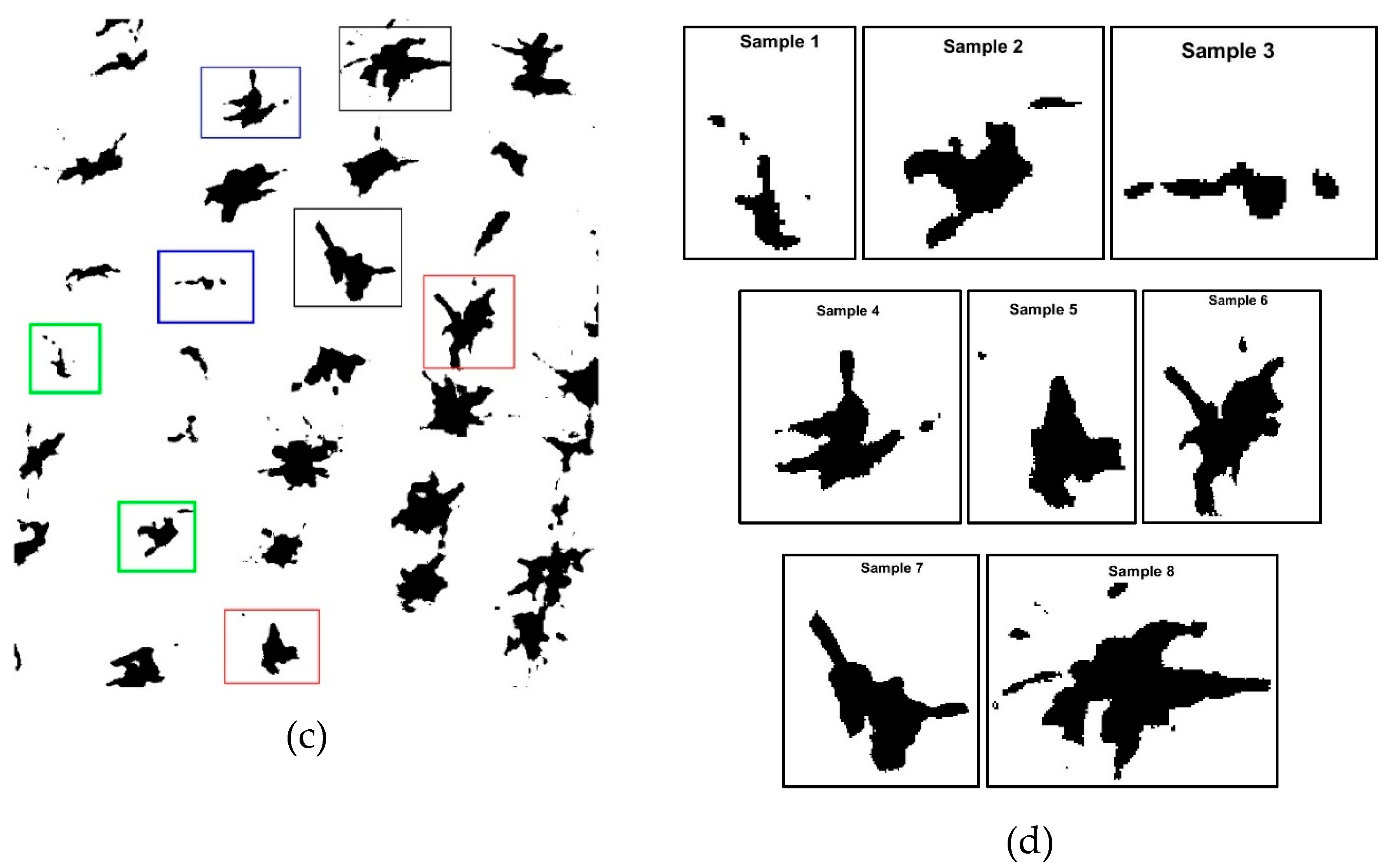
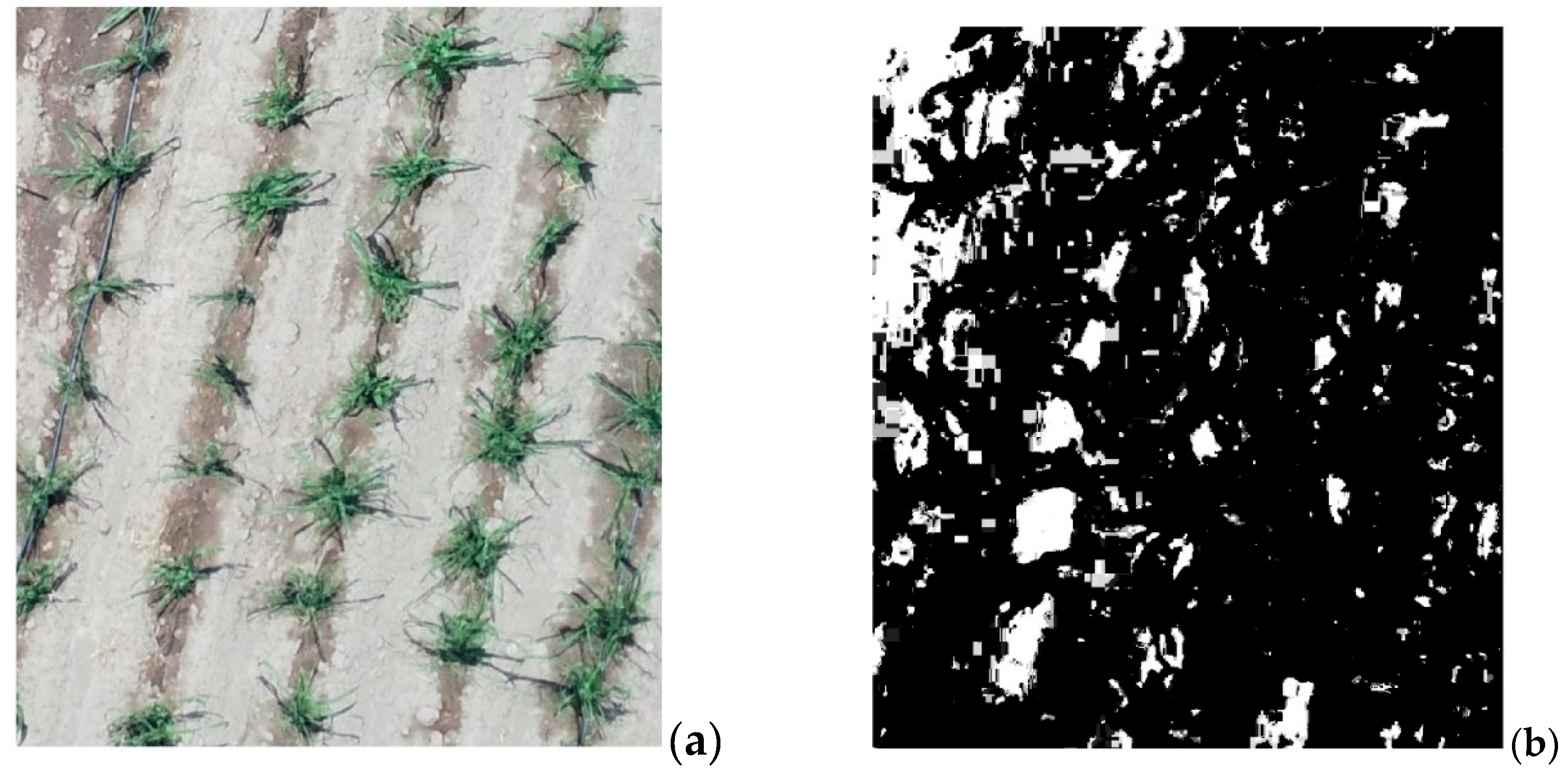
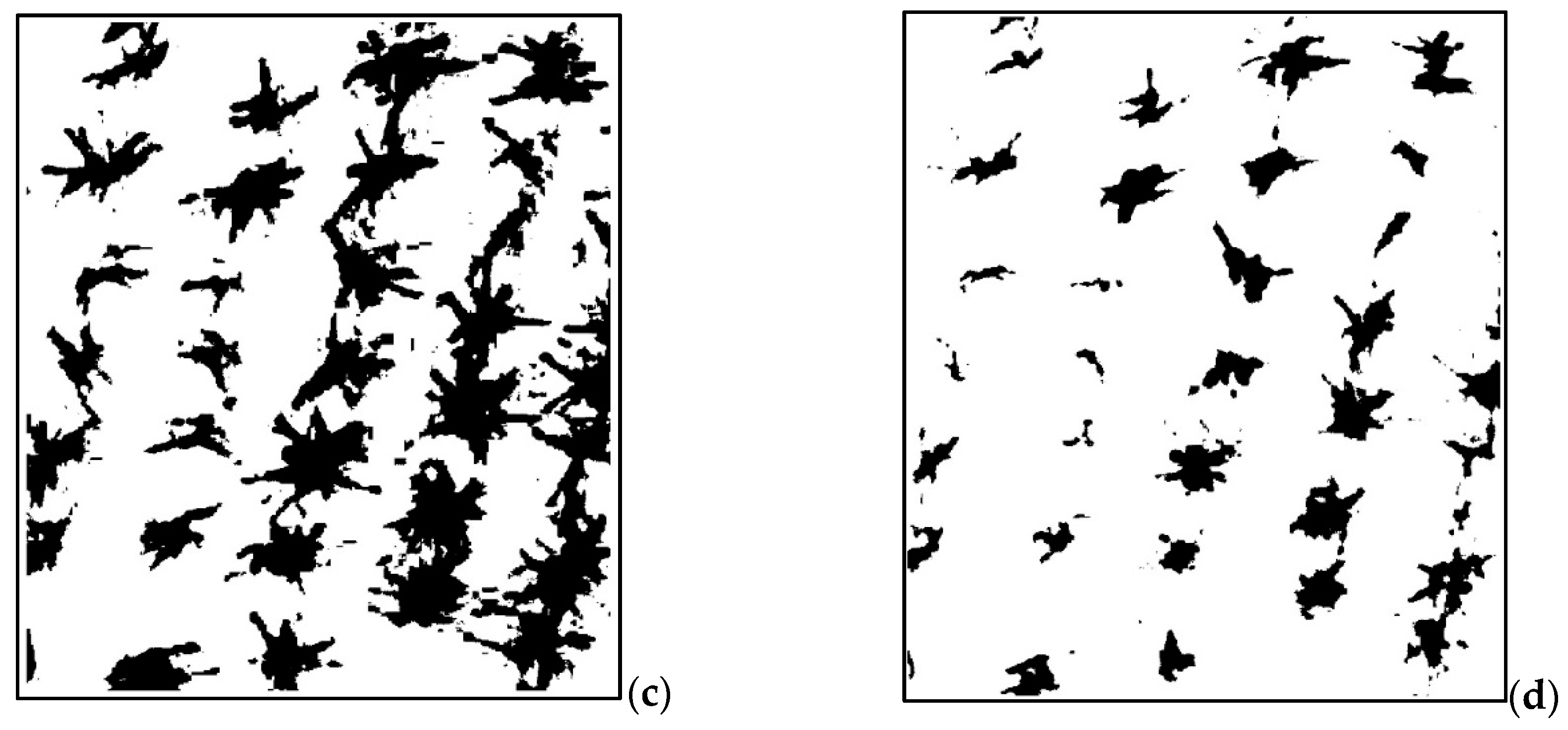
2.3. Image Color Pre-Processing

The images taken by the sensors mounted on the unmanned aerial vehicle were registered in the RGB color space. The L*a*b* color space also referred to as CIELAB, is one of the color spaces that least depends on illumination and pretends to emulate how humans perceive color. The colors in this space are located more intuitively, it being one of the most popular and uniform color spaces used to evaluate the color of an object [41]. It was developed by the Commission internationale de l’éclairage (International Commission of Illumination) (CIE). The L* value is the component that represents luminosity of color (low L* values indicate little brightness, while high L* values indicate high brightness). The a* parameter represents color in the red-green axis in a [−86.1367, 98.2964] range (+a indicates red, −a indicates green). The b* parameter represents color in the yellow-blue axis in a [−107.8650, 94.4756] range (+b indicates yellow, −b indicates blue). In order to transform the RGB color space to CIELAB, Equation (1) is used to transform to the CIEXYZ space [47,48].
[ X Y Z ] = [ 0.490   0.310   0.200 0.177   0.813   0.011 0.000   0.010   0.990 ] [ R G B ] ,
In the X, Y, Z space, luminosity is transformed through Equation (2):
L * = { 116 ( Y Y n ) 1 / 3 16 ,   s i   Y Y n > 0.008856 903.3 ( Y Y n ) 1 / 3   s i   Y Y n < 0.008856 ,
Parameters a* and b* are obtained through Equations (3) and (4):
a * = 500 [ f ( X X n ) f ( Y Y n ) ] ,
b * = 200 [ f ( Y Y n ) f ( Z Z n ) ] ,
where f(t) = t1/3 for t > 0.008856 and f(t) = 7.787t + 16/116 for t < 0.008856. Xn, Yn, Zn are the values for white, referencing the illuminator/observed used.
The images that were captured, registered and processed by the sensors in the RGB color space were transformed to the CIELAB color space for each orthomosaic. Once the images were transformed to the CIELAB color space, we got three available channels: L*, a* and b*. The value of the radiation that was absorbed, transmitted and reflected among the vegetation depended on its wavelength and the absorption selectivity of the pigments in the leaves—which may be characteristic of the species or caused by diseases or nutrient deficiencies [49]. Reflectance in the green channel in the interval of the electromagnetic spectrum is reflected by photosynthesis in leaves, for which reason vegetation is observed as green in the visible spectrum. The reflectance spectrum of green vegetation shows absorption peaks around 420 nm (violet), 490 nm (blue) and 660 nm (red). These are caused by strong absorption by chlorophyll [49]. For this study, we used channel a*, which represents color in the green-red axis in a [−86.1367, 98.2964] range (+a indicates red, −a indicates green). Vegetation is represented as green in the visible spectrum; thus, we proceed to filter the negative pixels in the a* channel of the CIELAB space to separate vegetation. The segmentation of the green pixels was done with MATLAB (Mathworks, Natik, MA, USA).

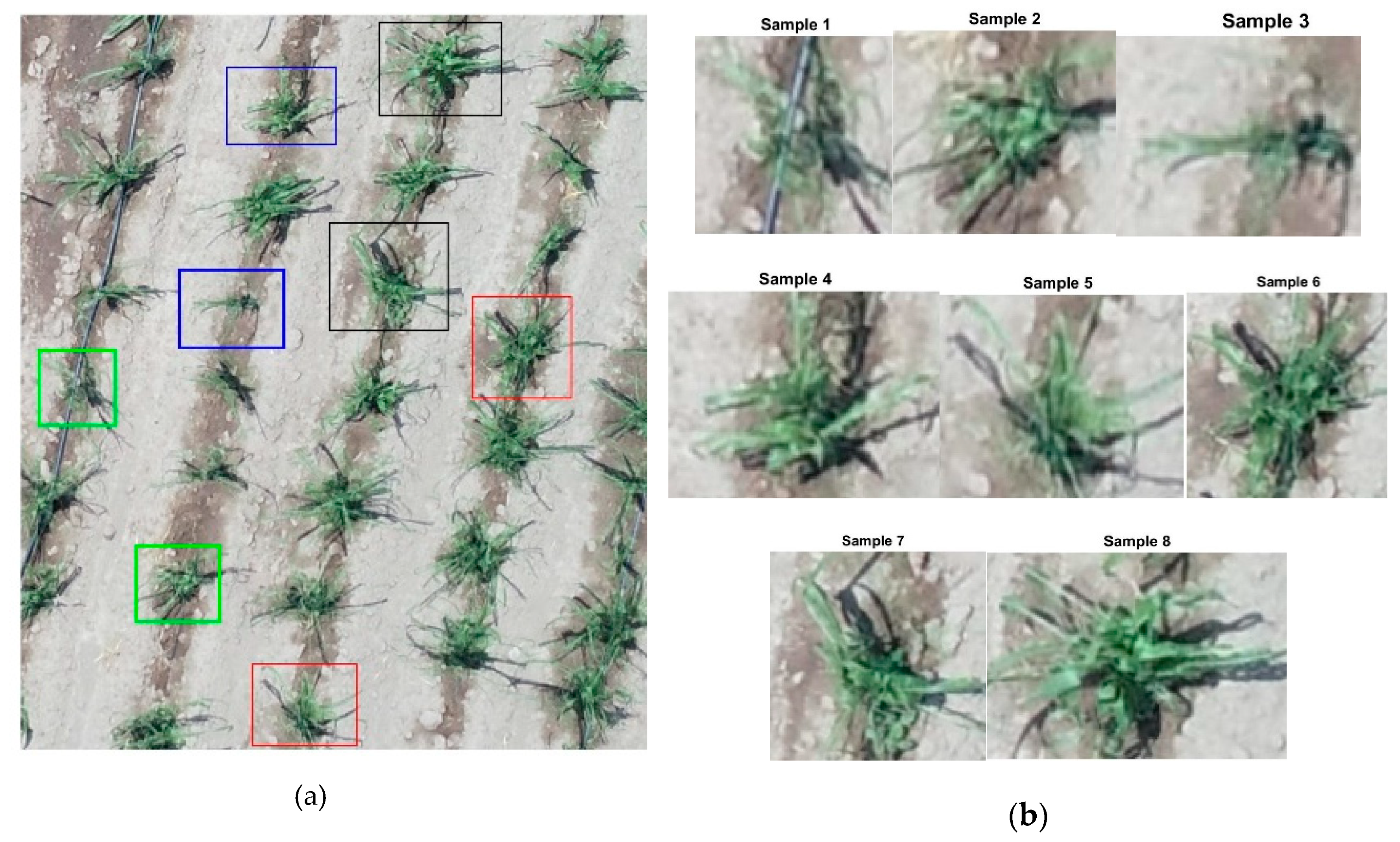
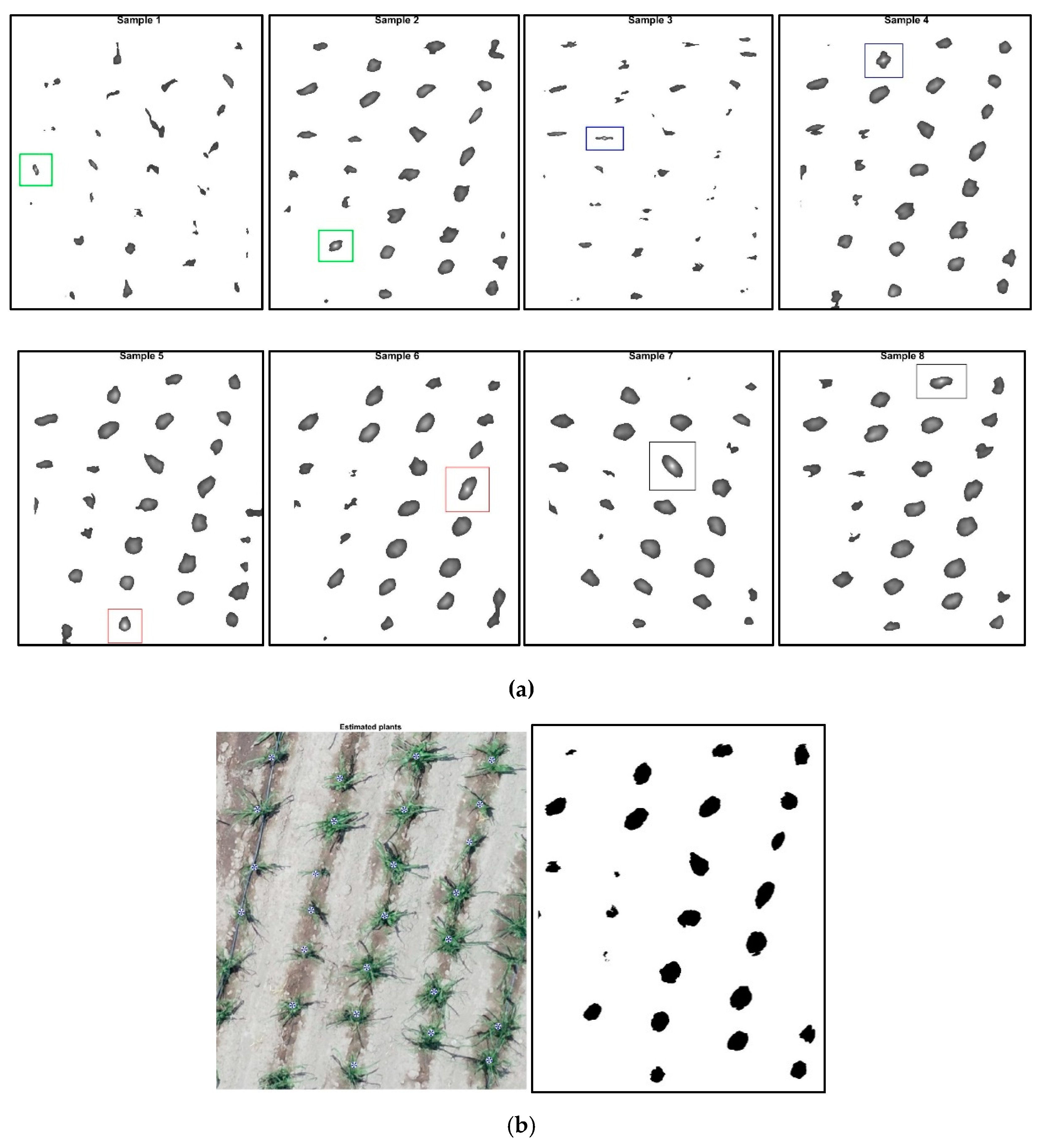
2.4. Selection of Samples or Templates (Plants)

In this stage, representative plants in the image are selected; these must be distinctive and with good quality. The selected plants must be distinguishable in the image and without overlap with other plants. Four, eight and twelve samples were selected based on the size or diameter of the corn plants, in pixels, in the image; two for small plants, two for large plants, with respect to those present in the image and the remaining four and eight for intermediate sizes in the different sample sizes. This means that it resulted in a total of 80, 160 and 240 samples for each flight date (Figure 2).

2.5. Normalized Cross Correlation

In the coincidence of the templates, understood as a technique to classify objects, a template or image sample is used; the general image is scanned to find the sample image through normalized cross-correlation. Correlation is a measure of the degree to which two variables or signals agree, not necessarily in real values but rather in the general performance of the same variables or signals; the two variables in the case of the images being the values of the corresponding pixels in both images (master and image) [45]. Correlation is an important tool in image processing, pattern recognition and other characteristics between two signals (cross-correlation); it is a standard approach to detect characteristics or patterns. The energy in an image shows variations, so cross-correlation between a characteristic and a region, both exactly equal, can fail. This also depends on the size of the template or sample. The correlation coefficient overcomes these difficulties by normalizing the image and the characteristics vectors to a longitude unit, producing a correlation coefficient similar to the cosine [50]. Comparison algorithms based on correlation techniques can directly use the images without any previous step to extract characteristics [51]. Normalized cross-correlation is a method commonly used to find 2D patterns in images from a template or sample T of (2 h + 1) × (2 W + 1) correlated to an image X. In locating the image (u,v), correlation is calculated through Equation (5) as:
C ( u , v ) = x , y [ f ( x , y ) f u , v ¯ ] [ t ( x u ,   y v ) t ¯ ] { x , y [ f ( x , y ) f u , v ¯ ] 2 x , y [ t ( x u ,   y v ) t ¯ ] 2 } 1 / 2 ,
where: f is the image, t ¯ is the template mean and f(u,v) is the mean of f(x,y) in the region under the template.
Normalized cross-correlation between the a* channel—where we filtered the green color and the selected samples—was done with Matlab, using the normxcorr2 function and command for each of the samples, obtaining an equal number of normalized cross-correlation matrices. In the resulting correlation images, we obtained values between −1 and +1, where the +1 value represented the selected sample and values under +1 represent certain coincidence with the master or correlated sample. Thus, a segmentation of the correlation coefficients was done, filtering values greater than the maximum correlation divided by four, which represents positive values (direct correlation) over 25% of the filtered sample. Once the correlation matrices between samples and the a* channel were filtered, we obtained the mean of the filtered matrices in a new means matrix. This matrix was then subjected to a new filtering process where values over 1/3 (0.33) were filtered from the means correlation matrix.

2.6. Description of the Analysis Process and Plant Counting

During plant counting and their distribution in the cropland, the plants are required to be free of weeds and in a development stage when there is no overlap yet. The orthomosaics generated from the images taken by the drone were used in the counting process, in which only the crop area was outlined in the orthomosaics using the ImageJ program (Wayne Rasband, NIH, Bethesda, MD, USA) in 20 plots.
To identify the objects extant in the images, it was necessary to differentiate the regions through a component labeling technique in binary images, assigning a label (1,2,3–i) to a subset of points that commonly integrate objects. The condition for a pixel to belong to a region is that it must be connected to the said region [40]. In the process of cross-correlation and obtainment of the correlation mean of the samples; the resulting matrix is a binary image (1 for white and 0 for black). Though Matlab, labeling was done for objects connected to 8, which in this case, are the plants identified through cross-correlation and filtered based on a mean correlation of sampler greater than the maximum (correlation matrix)/5 of the maximum positive correlation found in the process. The perimeter of the objects was used as a parameter to filter connected objects and only extract those that are plants.

2.7. Data Analysis

Twenty plots per image—120 m2 each—were processed for each orthomosaic on three flight dates (23, 44 and 65 days after sowing) during crop development, resulting in a total of 60 polygons. The count of the number of plants through the cross-correlation method for each polygon and sensor was registered in a table. The precision of the plant count obtained through normalized cross-correlation was compared against a manual count done for all 60 polygons in the experiment with the established corn crop at different stages.
As a validation of the automatic count through the normalized cross-correlation, it was compared against a manual count done in each of the 20 outlined plots using the root mean square error (RMSE) through Equation (9), mean absolute error (MAE), precision in the estimation (Ps) (Equation (6)), correlation coefficient (r) and determination coefficient (r2).
Ps = (Estimated plants)/(Counted plants),
Es = (Estimated plants − Counted plants)/(Counted plants),
M A E = 1 N i = 1 N | ( E s ) i | ,
R M S E = i = 1 N ( E s t i m a t e d   p l a n t s     C o u n t e d   p l a n t s ) 2 N ,
r2 = (σij2)/(σi × σj),
where N is the number of validated plots, |(Es)i| is the absolute of Es of the ith validation, σi is the standard deviation and σij is the covariance of the estimated and counted values.

3. Results and Discussion

Counting was done at 23, 44 and 67 days after sowing the corn plants through normalized cross-correlation, with four, eight and twelve samples in 20 outlined zones of the processed orthomosaics of the images taken by the sensor mounted on the UAV. The results are shown below.

3.1. Normalized Cross Correlation in Counting Corn Plants

The conversion of the RGB images into the CIELAB color space separated the green pixels in the a* channel in the image corresponding to vegetation pixels (plants). In the image filtering process, a threshold was used to separate the pixels into two types: vegetation and ground. The threshold (u) used was u = mean (a*) + mean (a*)/4 (Figure 2 and Figure 3). The edge in the mean (a+) threshold, according to the histogram of channel a*, places us at the pixels corresponding to the green color when adding 25% (mean (a+)/4); it places us in the histogram in the zone of greener pixels. When doing the extraction through the threshold, if the selected threshold is located in the green zone in channel a* in the color histogram, it allows us to do stronger filtering, thus separating overlapping plants; however, smaller plants and those with few leaves are eliminated, thus causing a lower estimation of the number of plants. This makes the selection of the threshold a key factor in vegetation extraction.
Having grouped the pixels into two types, the normalized cross-correlation (NCC) was done for four, eight and twelve samples (Table 2). When selecting the sample plants, it was important to take into account the representation of all plant shapes and sizes within the image to obtain good results in the counting through correlation. An important aspect that happens in the sample selection is if a small plant is selected as a sample, when the correlation is done with a plant twice the area size or more in the image, an overestimation error is made in the count.
In the plant counting process through the labeling of connected regions (Figure 4), one criterion to classify whether or not a region belongs to a plant is through the area in pixels in the image, hence the area of the corn plant was obtained from the selected samples (Figure 2 and Figure 3). The criterion was to select the area of the smallest plant in the samples, minus 20% of the area of the smallest plant; then, areas of this size or larger were considered as corn plants. In contrast, smaller areas were not considered as plants.
In the automatic counting of plants 44 DAS, images were taken with three different RGB sensors (Sequoia_4.9_4608 × 3456, FC6310_8.8_5472 × 3648 and Canon PowerShot S100_5.2_4000 × 3000), resulting in orthomosaics with a pixel size (ground sample distance—GSD) of 0.53, 0.49 and 0.88 cm, with respect to the image taken by the sensor (Table 2 and Figure 5). Precision in the automatic counting of plants was over 90% for all three resolutions of the three sensors and different sample sizes. A precision over 99% was obtained for twelve samples in the automatic counting through NCC in the case of orthomosaics generated with the FC6310_8.8_5472 × 3648 camera/sensor with a pixel size of 0.49 cm, with a determination coefficient r2 = 0.90, which has good data fit, root mean square error RMSE = 6.6 and mean absolute error MAE = 2.2%; with a mean planting density of 5 plants x m2. According to Table 2, bigger errors and lower precision were present when only 4 samples were selected, with corresponding greater precision and lower error with a larger sample selection. The sensor which presented the greatest error in the counting at different sample sizes (8.2, 8.6 and 7.5%) was the Canon PowerShotS100_5.2_4000 × 3000 with a pixel size (GSD) of 0.88 cm. Another important aspect in the correlation and selection of four, eight and twelve samples, is the computer processing time; four samples having a lower processing cost than the processing time needed for twelve samples.

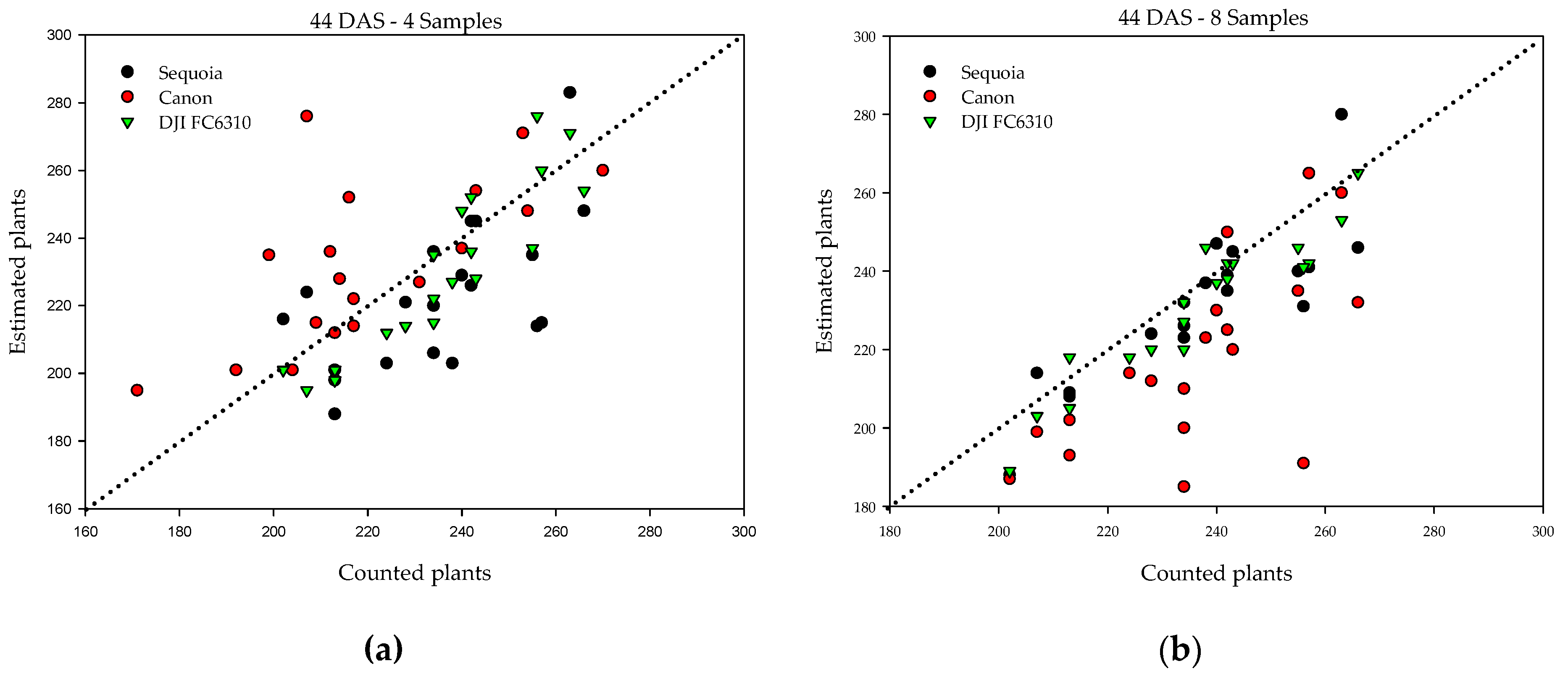
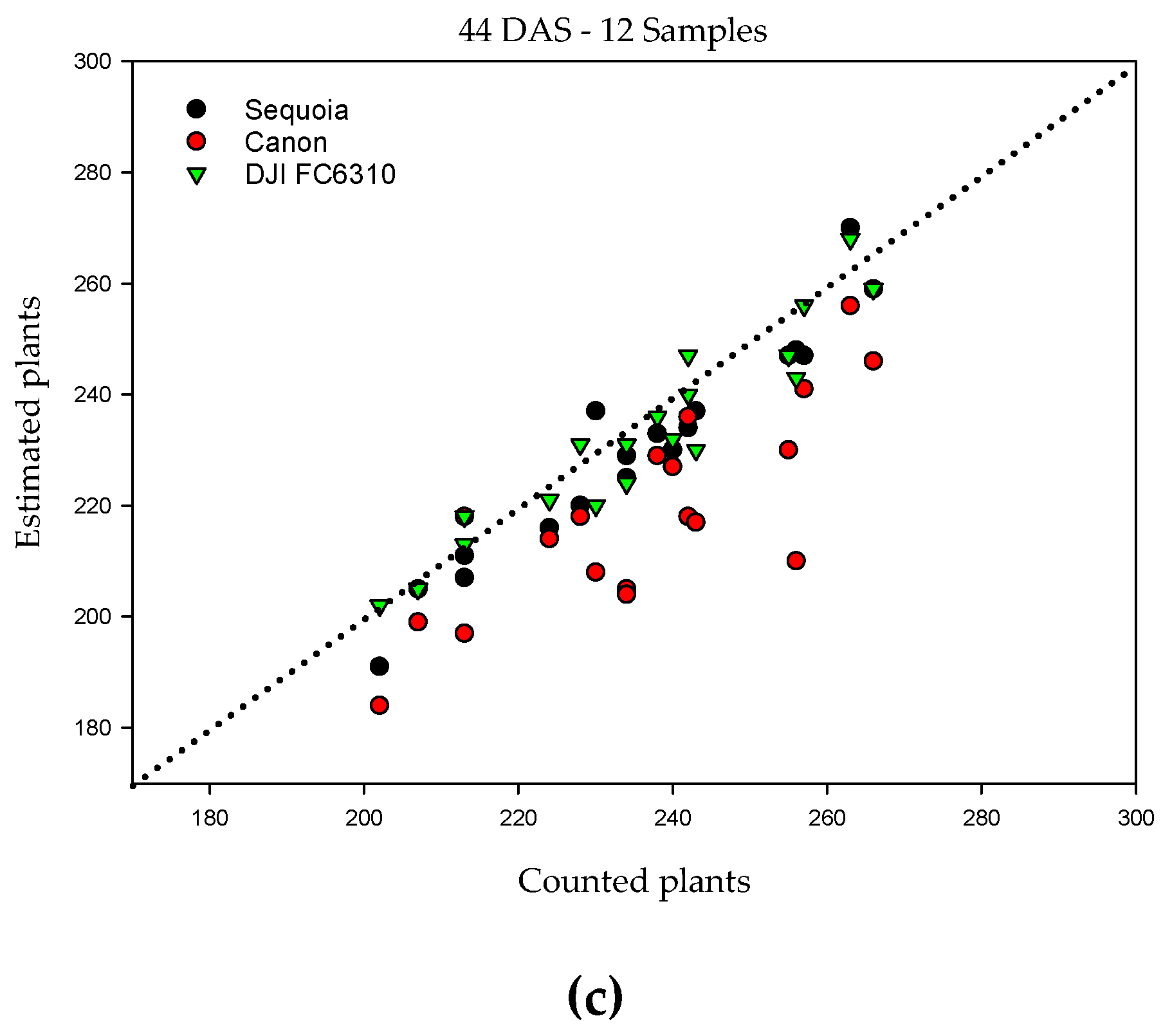
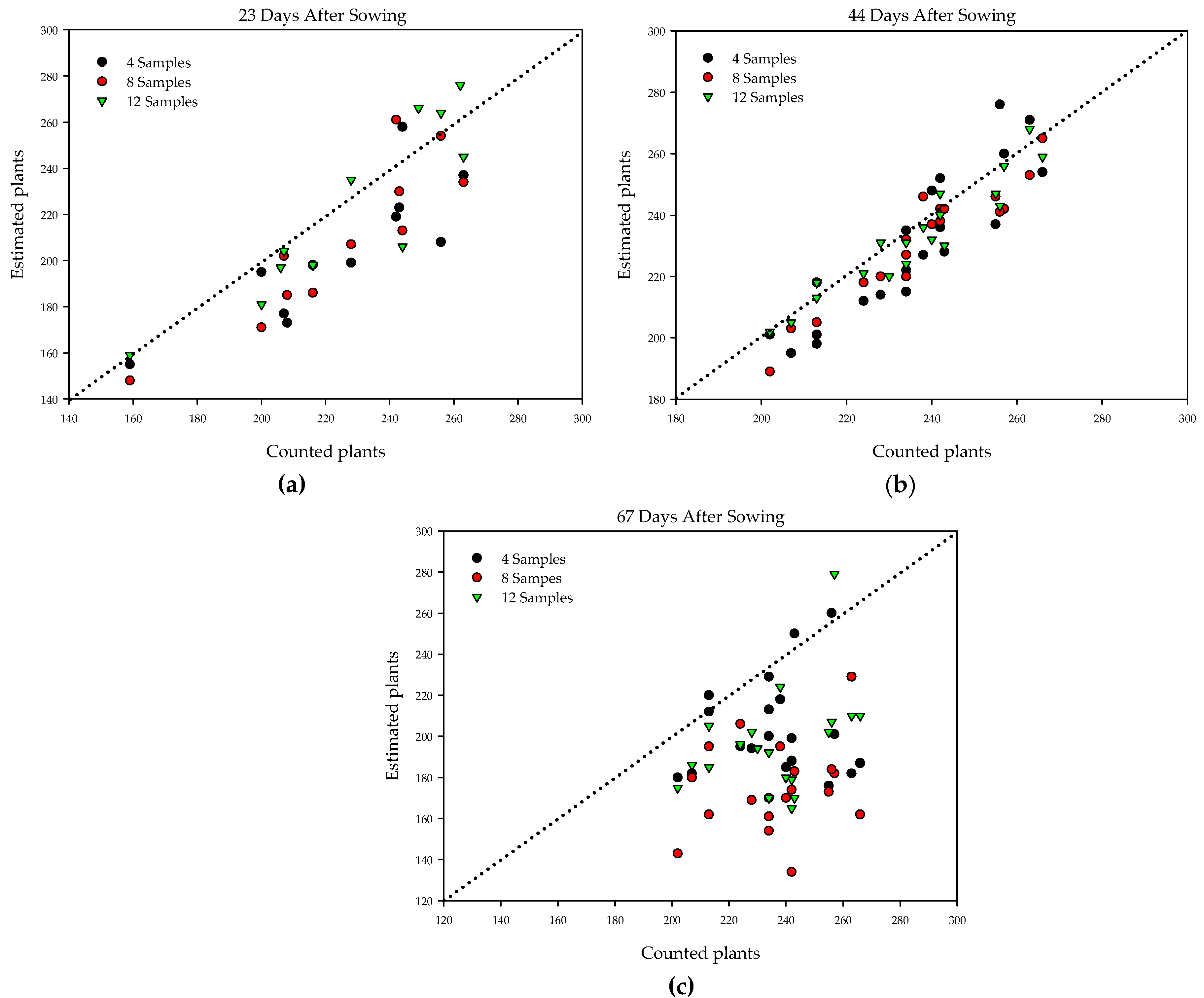
3.2. Precision in Plant Counting

Table 3 and Figure 6 show the results, which in turn show a lower error (2.2%–11%) in the counting for different sample sizes through NCC for 23 and 44 DAS (V2, V5 stage). Meanwhile, for larger plant size, at 67 DAS (V9 stage), the error in counting increases (14.2%–17.6%). The best precision (95%–98%) and lowest error (4.7%–2.2%) in counting were at 44 DAS when the plants had emerged but not yet overlapped. The lowest precision (74%) and highest error (25.7%) at 67 DAS were generated because the plants overlapped, thus making them impossible to separate in the filtering process by area, based on the sample plant. A better counting could be achieved through a process of separating the green pixels, increasing the green color filter. Similar errors are mentioned by Gnädinger and Schmidhalter [22]. In the case of 23 DAS, there were some zones where the plants were still in the emergence stage, thus in the filtering process by plant area, the plants in the emergence stage showed a too small pixel area and were therefore discarded in the filtering process.

4. Discussion

The development of unmanned aerial vehicles technology and its potential application for agriculture afforded by the spatial precision with which data can be obtained and the temporal availability of these data—together with precision agriculture—can facilitate differentiated management of crops, based on the knowledge of the variability extant in agricultural exploitation. Therefore, studies have been recently realized involving counting of cotton, rapeseed, sunflower, corn, potato and wheat plants [22,23,24,25,26].
The use of samples or templates in normalized cross-correlation (NCC) in counting corn plants is a relatively simple method to implement. This method gives the operator the selection of samples for counting based on the available images of the corn crops. Doing counting with RGB images enables the method to be implemented without the use of special sensors with special characteristics. This is an important factor with regard to the cost of the sensor, as sensors in the RGB color space are less expensive and more accessible. The results obtained in counting through samples and NCC are easy to interpret, since the obtained results can be visualized and verified quite promptly and exported to a geographical information system, overlaying it on the RGB image.
Another important aspect of NCC counting is the presence of weeds in the crops, which would result in a higher count in the number of plants that are present in the crop. Peña et al. [52] developed an image analysis process based on objects to discriminate corn crops from weeds. Some other methods use color and shape to identify weeds and separate plants [53,54]. In the established crop, manual and chemical control of weeds was undertaken, thus there was no perturbation associated to weeds in the counting done. In the obtained results, there was only an effect on counting from two overlapping plants, especially at 67 DAS (V9 stage), when the plants show greater coverage and leaf area. Counting corn plants through normalized cross-correlation in the first stages of corn crops grants significant savings in time and money when monitoring, following-up and carrying out the cultural labors of corn crops. This is true in the small and large scale, as well as in experiments where plant counting is a required phenotypic characteristic. It is also useful in modeling and estimating crop yield.

5. Conclusions

In the present study, automatic counting of corn plants through comparing templates with normalized cross-correlation (NCC) was done and validated. This was done in the first growth stages of the crop using RGB images acquired with an unmanned aerial vehicle. Automatic counting with template comparison through NCC resulted in a counting precision of over 90% up to 44 days after sowing (V5 stage), with 99% precision at 44 DAS with 12 templates (samples)/120 m2. With regard to pixel size (ground sample distance, GSD) and sensors, the precision in the estimation increased as the sensor resolution increased, resulting in precision over 97% and a mean error of 2.2%. The results indicate that UAV technology and template comparison through NCC provide good results in corn- plant counting during the early development stages of the crop, offering a good estimation of planting density in the crop. This facilitates field data compilation with high precision.

Author Contributions

H.F.-M. conceived the idea of the research, was in charge of the research, did the review of the article; H.G.-M. did the data review and collection, as well as the data analysis and the writing of the article; A.K.-G., R.A.-H., L.T.-C., M.A.V.-P. and O.R.M.-V. contributed to the analysis and review of the article. All authors have read and agreed to the published version of the manuscript.

Funding

This research received no external funding.

Acknowledgments

We thank the financial support of the Colegio de Postgraduados and the National Council of Science and Technology of Mexico (CONACyT) to make possible this study.

Conflicts of Interest

The authors declare no conflict of interest.

References

  1. Lunven, P. El Maiz en la Nutrición Humana; Organización de las Naciones Unidas para la Agricultura y la Alimentación: Roma, Italy, 1993. [Google Scholar]
  2. Assefa, Y.; Prasad, P.; Carter, P.; Hinds, M.; Bhalla, G.; Schon, R.; Jeschke, M.; Paszkiewicz, S.; Ciampitti, I.A. Yield responses to planting density for us modern corn hybrids: A synthesis-analysis. Crop. Sci. 2016, 56, 2802–2817. [Google Scholar] [CrossRef]
  3. Tollenaar, M. Is low plant density a stress in maize? Low Plant Density Stress Maize 1992, 37, 305–311. [Google Scholar]
  4. Ciampitti, I.A.; Camberato, J.J.; Murrell, S.T.; Vyn, T.J. Maize nutrient accumulation and partitioning in response to plant density and nitrogen Rate: I. macronutrients. Agron J. 2013, 105, 783–795. [Google Scholar] [CrossRef] [Green Version]
  5. Yang, G.; Liu, J.; Zhao, C.; Li, Z.; Huang, Y.; Yu, H.; Xu, B.; Yang, X.; Zhu, D.; Zhang, X.; et al. Unmanned Aerial Vehicle Remote Sensing for Field-Based Crop Phenotyping: Current Status and Perspectives. Front. Plant Sci. 2017, 8, 1111. Available online: https://www.frontiersin.org/articles/10.3389/fpls.2017.01111/full (accessed on 4 February 2020). [CrossRef]
  6. Torres-Sánchez, J.; Peña, J.M.; de Castro, A.I.; López-Granados, F. Multi-temporal mapping of the vegetation fraction in early-season wheat fields using images from UAV. Comput. Electron. Agric. 2014, 103, 104–113. [Google Scholar] [CrossRef]
  7. Zhang, C.; Kovacs, J.M. The application of small unmanned aerial systems for precision agriculture: A review. Precis Agric. 2012, 13, 693–712. [Google Scholar] [CrossRef]
  8. Hengl, T. Finding the right pixel size. Comput. Geosci. 2006, 32, 1283–1298. [Google Scholar] [CrossRef]
  9. Nex, F.; Remondino, F. UAV for 3D mapping applications: A review. Appl. Geomat. 2014, 6, 1–15. [Google Scholar] [CrossRef]
  10. Torres-Sánchez, J.; López Granados, F.; Castro AI de Peña Barragán, J.M. Configuration and specifications of an unmanned aerial vehicle (UAV) for early site specific weed management. PLoS ONE 2013. [Google Scholar] [CrossRef] [Green Version]
  11. Peña, J.M.; Torres-Sánchez, J.; Serrano-Pérez, A.; De Castro, A.I.; López-Granados, F. Quantifying efficacy and limits of Unmanned Aerial Vehicle (UAV) technology for weed seedling detection as affected by sensor resolution. Sensors 2015, 15, 5609–5626. [Google Scholar] [CrossRef] [Green Version]
  12. Koh, J.C.O.; Hayden, M.; Daetwyler, H.; Kant, S. Estimation of crop plant density at early mixed growth stages using UAV imagery. Plant Methods 2019, 15, 64. [Google Scholar] [CrossRef] [PubMed]
  13. Colomina, I.; Molina, P. Unmanned aerial systems for photogrammetry and remote sensing: A review. ISPRS J. Photogramm. Remote Sens. 2014, 92, 79–97. [Google Scholar] [CrossRef] [Green Version]
  14. Yao, H.; Qin, R.; Chen, X. Unmanned aerial vehicle for remote sensing applications—A review. Remote Sens. 2019, 11, 1443. [Google Scholar] [CrossRef] [Green Version]
  15. Maes, W.H.; Steppe, K. Perspectives for remote sensing with unmanned aerial vehicles in precision agriculture. Trends Plant Sci. 2019, 24, 152–164. [Google Scholar] [CrossRef]
  16. López-Granados, F.; Torres-Sánchez, J.; De Castro, A.-I.; Serrano-Pérez, A.; Mesas-Carrascosa, F.-J.; Peña, J.-M. Object-based early monitoring of a grass weed in a grass crop using high resolution UAV imagery. Agron. Sustain. Dev. 2016, 36, 67. [Google Scholar] [CrossRef]
  17. Holman, F.H.; Riche, A.B.; Michalski, A.; Castle, M.; Wooster, M.J.; Hawkesford, M.J. High Throughput field phenotyping of wheat plant height and growth rate in field plot trials using uav based remote sensing. Remote Sens. 2016, 8, 1031. [Google Scholar] [CrossRef]
  18. Maresma, Á.; Ariza, M.; Martínez, E.; Lloveras, J.; Martínez-Casasnovas, J.A. Analysis of vegetation indices to determine nitrogen application and yield prediction in maize (Zea mays L.) from a standard UAV service. Remote Sens. 2016, 8, 973. [Google Scholar] [CrossRef] [Green Version]
  19. Madec, S.; Baret, F.; De Solan, B.; Thomas, S.; Dutartre, D.; Jezequel, S.; Hemmerlé, M.; Colombeau, G.; Comar, A. High-throughput phenotyping of plant height: Comparing unmanned aerial vehicles and ground LiDAR estimates. Front. Plant Sci. 2017, 8. [Google Scholar] [CrossRef] [Green Version]
  20. Marcial, M.D.J.; Gonzalez-Sanchez, A.; Jimenez-Jimenez, S.I.; Ontiveros-Capurata, R.E.; Ojeda-Bustamante, W. Estimation of vegetation fraction using RGB and multispectral images from UAV. Int. J. Remote Sens. 2019, 40, 420–438. [Google Scholar] [CrossRef]
  21. Liu, S.; Baret, F.; Andrieu, B.; Burger, P.; Hemmerlé, M. Estimation of Wheat Plant Density at Early Stages Using High Resolution Imagery. Front. Plant Sci. 2017. Available online: https://www.frontiersin.org/articles/10.3389/fpls.2017.00739/full (accessed on 4 February 2020). [CrossRef] [Green Version]
  22. Gnädinger, F.; Schmidhalter, U. digital counts of maize plants by Unmanned Aerial Vehicles (UAVs). Remote Sens. 2017, 9, 544. [Google Scholar] [CrossRef] [Green Version]
  23. Zhao, B.; Zhang, J.; Yang, C.; Zhou, G.; Ding, Y.; Shi, Y.; Zhang, N.; Xie, J.; Liao, Q. Rapeseed seedling stand counting and seeding performance evaluation at two early growth stages based on unmanned aerial vehicle imagery. Front. Plant Sci. 2018, 9, 1362. [Google Scholar] [CrossRef] [PubMed]
  24. Chen, R.; Chu, T.; Landivar, J.; Yang, C.; Maeda, M. Monitoring cotton (Gossypium hirsutum L.) germination using ultrahigh-resolution UAS images. Precis. Agric. 2017, 19, 1–17. [Google Scholar] [CrossRef]
  25. Sankaran, S.; Quirós, J.J.; Knowles, N.R.; Knowles, L.O. High-resolution aerial imaging based estimation of crop emergence in potatoes. Am. J. Potato Res. 2017, 94, 658–663. [Google Scholar] [CrossRef]
  26. Jin, X.; Liu, S.; Baret, F.; Hemerlé, M.; Comar, A. Estimates of plant density of wheat crops at emergence from very low altitude UAV imagery. Remote Sens. Environ. 2017, 198, 105–114. [Google Scholar] [CrossRef] [Green Version]
  27. Zhang, J.; Basso, B.; Richard, F.P.; Putman, G.; Shuai, G. Estimating Plant Distance in Maize Using Unmanned Aerial Vehicle (UAV). Available online: https://www.ncbi.nlm.nih.gov/pmc/articles/PMC5909920/ (accessed on 16 March 2020).
  28. Shuai, G.; Martinez-Feria, R.A.; Zhang, J.; Li, S.; Price, R.; Basso, B. Capturing maize stand heterogeneity across yield-stability zones using Unmanned Aerial Vehicles (UAV). Sensors 2019, 19, 4446. [Google Scholar] [CrossRef] [PubMed] [Green Version]
  29. Kitano, B.T.; Mendes, C.C.T.; Geus, A.R.; Oliveira, H.C.; Souza, J.R. Corn plant counting using deep learning and UAV images. IEEE Geosci. Remote Sens. Lett. 2019, 1–5. [Google Scholar] [CrossRef]
  30. Ribera, J.; Chen, Y.; Boomsma, C.; Delp, E.J. Counting plants using deep learning. In Proceedings of the 2017 IEEE Global Conference on Signal and Information Processing (GlobalSIP), Montreal, QC, Canada, 14–16 November 2017. [Google Scholar] [CrossRef]
  31. Wang, C.; Guo, X.; Zhao, C. Detection of corn plant population and row spacing using computer vision. In Proceedings of the 2011 Second International Conference on Digital Manufacturing Automation, Zhangjiajie, China, 5–7 August 2011; pp. 405–408. [Google Scholar] [CrossRef]
  32. Gracia-Romero, A.; Kefauver, S.; Vergara-Díaz, O.; Zaman-Allah, M.; Prasanna, B.M.; Cairns, J.E.; Araus, J.L. Comparative performance of ground vs. aerially assessed RGB and multispectral indices for early-growth evaluation of maize performance under phosphorus fertilization. Front. Plant Sci. 2017, 8. [Google Scholar] [CrossRef] [Green Version]
  33. Guerrero, J.M.; Pajares, G.; Montalvo, M.; Romeo, J.; Guijarro, M. Support Vector Machines for crop/weeds identification in maize fields. Expert Syst. Appl. 2012, 39, 11149–11155. [Google Scholar] [CrossRef]
  34. Guijarro, M.; Pajares, G.; Riomoros, I.; Herrera, P.J.; Burgos-Artizzu, X.P.; Ribeiro, A. Automatic segmentation of relevant textures in agricultural images. Comput. Electron. Agric. 2011, 75, 75–83. [Google Scholar] [CrossRef] [Green Version]
  35. Zaman-Allah, M.; Vergara, O.; Araus, J.L.; Tarekegne, A.; Magorokosho, C.; Zarco-Tejada, P.J.; Hornero, A.; Albà, A.H.; Das, B.; Craufurd, P.; et al. Unmanned aerial platform-based multi-spectral imaging for field phenotyping of maize. Plant Methods 2015, 11, 35. [Google Scholar] [CrossRef] [PubMed] [Green Version]
  36. Zhou, B.; Elazab, A.; Bort, J.; Vergara, O.; Serret, M.D.; Araus, J.L. Low-cost assessment of wheat resistance to yellow rust through conventional RGB images. Comput. Electron. Agric. 2015, 116, 20–29. [Google Scholar] [CrossRef]
  37. Diaz, O.V.; Zaman-Allah, M.; Masuka, B.; Hornero, A.; Zarco-Tejada, P.; Prasanna, B.M.; Cairns, J.E.; Araus, J.L. A novel remote sensing approach for prediction of maize yield under different conditions of nitrogen fertilization. Front. Plant Sci. 2016, 7. [Google Scholar] [CrossRef] [Green Version]
  38. Yousfi, S.; Kellas, N.; Saidi, L.; Benlakehal, Z.; Chaou, L.; Siad, D.; Herda, F.; Karrou, M.; Vergara, O.; Gracia, A.; et al. Comparative performance of remote sensing methods in assessing wheat performance under Mediterranean conditions. Agric. Water Manag. 2016, 164, 137–147. [Google Scholar] [CrossRef]
  39. Robertson, A.R. The CIE 1976 color-difference formulae. Color Res. Appl. 1977, 2, 7–11. [Google Scholar] [CrossRef]
  40. Mendoza, F.; Dejmek, P.; Aguilera, J.M. Calibrated color measurements of agricultural foods using image analysis. Postharvest Biol. Technol. 2006, 41, 285–295. [Google Scholar] [CrossRef]
  41. Macedo-Cruz, A.; Pajares, G.; Santos, M.; Villegas-Romero, I. Digital image sensor-based assessment of the status of oat (Avena sativa L.) crops after frost damage. Sensors 2011, 11, 6015–6036. [Google Scholar] [CrossRef] [Green Version]
  42. Cheng, G.; Han, J. A survey on object detection in optical remote sensing images. ISPRS J. Photogramm. Remote Sens. 2016, 117, 11–28. [Google Scholar] [CrossRef] [Green Version]
  43. Tiede, D.; Krafft, P.; Füreder, P.; Lang, S. Stratified template matching to support refugee camp analysis in OBIA workflows. Remote Sens. 2017, 9, 326. [Google Scholar] [CrossRef] [Green Version]
  44. Nuijten, R.J.G.; Kooistra, L.; De Deyn, G.B. Using Unmanned Aerial Systems (UAS) and Object-Based Image Analysis (OBIA) for measuring plant-soil feedback effects on crop productivity. Drones 2019, 3, 54. [Google Scholar] [CrossRef] [Green Version]
  45. Ahuja, K.K.; Tuli, P. Object recognition by template matching using correlations and phase angle method. Int. J. Adv. Res. Comput. Commun. Eng. 2013, 2, 3. [Google Scholar]
  46. Kalantar, B.; Mansor, S.B.; Shafri, H.Z.M.; Halin, A.A. Integration of template matching and object-based image analysis for semi-automatic oil palm tree counting in UAV images. In Proceedings of the 37th Asian Conference on Remote Sensing, Colombo, Sri Lanka, 17–21 October 2016. [Google Scholar]
  47. Schanda, J. Colorimetry: Understanding the CIE System; John Wiley & Sons: Hoboken, NJ, USA, 2007. [Google Scholar]
  48. Recky, M.; Leberl, F. Windows Detection Using K-means in CIE-Lab Color Space. In Proceedings of the 20th International Conference on Pattern Recognition, Istanbul, Turkey, 23–26 August 2010; pp. 356–359. [Google Scholar] [CrossRef]
  49. Van Der Meer, F.D.; De Jong, S.M.; Bakker, W. Imaging Spectrometry: Basic Analytical Techniques. In Imaging Spectrometry: Basic Principles and Prospective Applications; Remote Sensing and Digital Image Processing; Springer: Dordrecht, The Netherlands, 2001; pp. 17–61. [Google Scholar] [CrossRef]
  50. Lewis, J.P. Fast Template Matching. In Proceedings of the Vision Interface 95, Quebec City, QC, Canada, 15–19 May 1995; pp. 120–123. [Google Scholar]
  51. Lindoso Muñoz, A. Contribución al Reconocimiento de Huellas Dactilares Mediante Técnicas de Correlación y Arquitecturas Hardware Para el Aumento de Prestaciones. February 2009. Available online: https://e-archivo.uc3m.es/handle/10016/5571 (accessed on 4 February 2020).
  52. Peña, J.M.; Torres-Sánchez, J.; de Castro, A.I.; Kelly, M.; López-Granados, F. Weed mapping in early-season maize fields using object-based analysis of Unmanned Aerial Vehicle (UAV) images. PLoS ONE 2013, 8. [Google Scholar] [CrossRef] [PubMed] [Green Version]
  53. Gée, C.H.; Bossu, J.; Jones, G.; Truchetet, F. Crop/weed discrimination in perspective agronomic images. Comput. Electron. Agric. 2008, 60, 49–59. [Google Scholar] [CrossRef]
  54. Swain, K.C.; Nørremark, M.; Jørgensen, R.N.; Midtiby, H.S.; Green, O. Weed identification using an automated active shape matching (AASM) technique. Biosyst. Eng. 2011, 110, 450–457. [Google Scholar] [CrossRef]
Figure 1. (a) Established corn experimental field; (b) Ground control points (GCP); (c) 3DR Solo UAV; (d) DJI Phantom UAV.
Agronomy 10 00469 g001
Figure 2. Selection of corn plant samples on the orthomosaic generated using the camera DJI FC6310. (a) Selection of samples in the RGB image; (c) Samples selected for counting in the a* channel; (b) Samples selected in the RGB image; (d) Samples with pre-processing in the a* channel of the CIELAB model.
Agronomy 10 00469 g002aAgronomy 10 00469 g002b
Figure 3. Green pixel filtering in channel a*, from left to right: (a) RGB image; (b) threshold = 0; (c) threshold = mean (a*); (d) threshold = mean (a*) + mean (a*)/4.
Agronomy 10 00469 g003aAgronomy 10 00469 g003b
Figure 4. (a) Binary images of the normalized cross-correlation of eight samples with respect to the image; (b) image resulting from the mean correlation of eight samples.
Agronomy 10 00469 g004
Figure 5. Corn plant count with respect to the sensor and pixel size 44 days after sowing (V5 stage). (a) correlation in the count for four samples; (b) correlation in the count for eight samples; (c) correlation in the count for twelve samples.
Agronomy 10 00469 g005aAgronomy 10 00469 g005b
Figure 6. Manual count and automatic count through NCC of corn plants at different days after sowing (DAS). (a) corn plant count at 23 DAS (V2 stage) through NCC; (b) corn plant count at 44 DAS (V5 stage) through NCC; (c) corn plant count at 67 DAS (V9 stage) through NCC.
Agronomy 10 00469 g006
Table 1. Flight log at different days after sowing (DAS).
DASDateDevelopment StagesSensorN° of ImagesArea (m2)Pixel Size
23April 27V2Sequoia_4.9_4608 × 3456 (RGB)4135450.56
44May 18V5Sequoia_4.9_4608 × 3456 (RGB)15763090.53
44May 18V5DJI FC6310_8.8_5472 × 3648 (RGB)27210,0670.49
44May 18V5CanonPowerShotS100_5.2_4000 × 3000 (RGB)12069770.88
67June 8V9CanonPowerShotS100_5.2_4000 × 3000 (RGB)8013,5431.05
Table 2. Precision (Ps) in corn plant count with respect to the sensor and pixel size 44 days after sowing (V5 stage).
SamplesPixel Size (cm)Ps (%)RMSErr2MAE (%)
40.539521.80.590.357.7
0.889322.90.740.548.2
0.499712.20.910.824.7
80.539811.50.860.743.9
0.889225.50.680.468.6
0.49988.40.940.893.0
120.53987.50.970.933.0
0.889320.60.810.657.5
0.49996.60.950.902.2
Table 3. Results between counting through the normalized cross-correlation and manual counting for the different cameras used during the corn growing season showing precision in the estimation (Ps), root mean square error (RMSE), correlation coefficient (r), determination coefficient (r2) and mean absolute error (MAE).
DASSensorSamplesPs(%)RMSErr2MAE (%)
23Sequoia_4.9_4608 × 3456 (RGB)49125.870.990.9811.0
89319.170.820.677.2
129713.170.880.774.7
44DJI FC6310_8.8_5472 × 3648 (RGB)495 112.240.910.824.7
8988.410.940.893.0
12986.610.950.902.2
67CanonPowerShotS100_5.2_4000 × 3000 (RGB)48743.050.080.0114.2
87493.150.230.0525.7
128346.620.400.1617.6

