Impact Analysis of Environmental Conditions on Odour Dispersion Emitted from Pig House with Complex Terrain Using CFD

Abstract

With the rise in livestock production, the odour concentration emitted from livestock facilities has significantly increased. For this reason, odour complaints have become a major issue. The dispersion of the odour into the atmosphere is affected by various factors (wind speed, wind direction, atmospheric stability, terrain condition, ventilation type, and so on). Thus, a thorough analysis on the factor influencing odour dispersion is necessary to establish regulations and policies for odour management. Therefore, this research aimed to evaluate odour dispersion generated from a pig house with complex terrain using computational fluid dynamics (CFD) and to statistically determine the key factor for odour dispersion. By comparing CFD-computed results with field-measured data, an appropriate grid size, time step, and turbulence model of the CFD model were determined. Considering various factors, case studies were performed using the validated CFD model. The CFD-computed results showed that odour dispersion distance at the level of 1 OU m⁻³ ranged from 129.7 to 1488.1 m. The prediction of odour dispersion distance varies with the change of factor being analysed. Finally, the statistical analysis showed that the most influential factor that affected odour dispersion distance was the wind speed with a t-value: −9.057.

1. Introduction

Pig production in the Republic of Korea accounts for 40% of the total livestock industry (USD 1.8 billion) in the country [1]. The number of pig farms was continuously reduced to 50.3% from 12,227 in 2005 to having only 6160 pig farms for the year 2019, but, the scale of pig rearing was significantly increased from 8,961,505 heads in 2005 to 11,317,000 heads in 2019 [2]. This indicates that pig farms have progressively been enlarged to meet the rise in meat demand. The increase in production intensified manure generation, causing an inevitable rise in the number of complaints related to odour emission. The number of complaints related to livestock odour upsurged to 27% from 4302 in 2005 to 6112 in 2017 [3].

To cope with this problem, the government has established policies to regulate and minimize the effect of odour in the vicinity of pig houses. This includes but not limited to the odour prevention law related to the allowable value of odour emission from livestock facilities and the establishment of setback distance. Research on odour management using physical and chemical methods has also been conducted. Past research has focused on studies to determine the optimum practice to minimize odour nuisance through field experiments [4,5,6]. Most studies mainly evaluated the efficiency of additives (chemical and biological methods) or abatement facilities (biofilters, liquid manure recharging systems, and so on) to reduce livestock odours [7,8,9,10,11,12,13,14,15]. These field experiment studies usually measured and evaluated single odorous gas such as ammonia (NH₃), hydrogen sulphide (H₂S), methane (CH₄), and carbon dioxide (CO₂). However, an evaluation of complex odour is also necessary because the odour concentration of individual single gas and the complex odour emitted from animal facilities are different. Furthermore, the odour causing a nuisance to the nearby community tends to be caused by a combination of two or more substances rather than a single substance.

Sensory evaluation (dynamic olfactometry method) is used to estimate the quantitative amount of complex odour at a specific location and time. Although this method can obtain the actual value in the field, multiple panels are required for the measurement. Despite the established guidelines for the selection and training of the sensory panel members, the different odour perception ability of each panel can contribute to the errors in measuring odour. Furthermore, the sensory evaluation method has several disadvantages such as difficulties in managing the samples and being time-consuming considering multipoint measurements [16,17]. For these reasons, the evaluation of odour dispersion outside livestock buildings using the sensory evaluation method was not intensively considered and was used only for evaluating the odour concentration present at a specific location. The influence of the distance between the source and the receptor must be considered to control the odour from the outside. The impact of the weather conditions on odour dispersion should also be taken into account, especially weather conditions such as wind speed, wind direction, and atmospheric stability, which have a great influence on dispersion. The field experiment study of Yeo et al. [18] measured complex odour using sensory evaluation and measured weather conditions. However, the conduct of odour field measurements required intensive labour and excessive cost, as it considered the effect of various meteorological conditions in the odour emission. Furthermore, due to the difficulties of controlling the environmental conditions, the results of the field measurement were only valid in a specific weather condition during the measurement period. To overcome these, numerical dispersion models that mathematically calculate the dispersion of pollutants into the atmosphere and change of pollutant concentration were developed and used in various studies [19,20]. However, like field experiments, numerical dispersion models also have limitations such that they have difficulty in imitating the actual dispersion trend when not properly modelled [21].

One of the widely used numerical analysis methods for predicting the dispersion of the odour is the Gaussian dispersion model [22,23,24,25,26,27,28,29,30]. This dispersion model assumes that the horizontal and vertical odour concentration in the plume has a normal distribution (Gaussian distribution). Owing to the required short calculation time of Gaussian dispersion models and simple calculation procedure, these dispersion models have been frequently used. Specifically, the Gaussian dispersion models were found to be effective in research studies where the main objective was to know the distance and concentration ranges of pollutants blown to the atmosphere by chimneys [31] and typically used in point source emissions [32]. However, when the mesh resolution for the Gaussian dispersion model was set to a very large grid, the odour concentration prediction of the model resulted in an overestimation of odour flow. In addition, in the Gaussian dispersion model, it was difficult to analyse the odour dispersion in detail by considering the local wind environment generated from the complex terrain and layout of livestock facilities. Other commonly used odour dispersion models were thoroughly discussed in the paper of Conti et al., 2020 [33].

In comparison, the numerical analysis of atmospheric odour dispersion using computational fluid dynamics (CFD) allowed more realistic simulation and can compensate for the limitations of the Gaussian dispersion model even though it required detailed geometry design and more computational time. The importance of CFD has been validated in many fields including industrial applications [34,35,36], environmental applications [37,38,39], and physiological applications [40,41]. Specifically, the application of CFD in the field of agriculture such as in odour transport [29,42,43,44,45,46,47] and dust emission [48] was recently conducted. However, these studies used flat or very small areas to simulate dispersion phenomena with CFD.

To accurately predict odour dispersion, it is necessary to consider the topographical effects in the target areas where the local wind environment is affected by complex terrain such as the mountainous area. Hence, recent research tried to simulated airflow analysis and the change of the odour concentration emitted from livestock buildings, taking into account the complex terrain in the computational domain [20,49]. Specifically, Hong et al. [20] developed and validated an initial CFD model with complex terrain to simulate the odour dispersion of the pig house, considering weather conditions such as atmospheric stability and wind direction. However, the paper assumed the odour source was area source and the odour that was emitted at the surface of the pig farm was considered as the odour source. Furthermore, these research studies mainly focused on analysing the trend of odour dispersion outside the pig house, and there was a lack of research on the analysis of key factors affecting the dispersion of odour in the atmosphere. For instance, Lin et al. [29] concluded that wind speed and wind direction have an impact on the dispersion of odour in the atmosphere. The same statement was made by Chastain [30], implying that the direction of prevailing wind and the presence of wind breaks must be considered in the model. The ventilation inside the pig farm also contributed to the amount of odour emitted from the livestock facilities. These factors were agreed by Capelli et al. [28], which emphasized in the manuscript the importance of meteorological information needed for dispersion modelling such as wind speed, wind direction, and atmospheric stability. In addition, Chastain [30] includes the influence of the topographical condition of the target farm. Papers such as those published by Ubeda et al. [50], Hong et al. [51], and Conti et al. [33] support the other claims of the previously mentioned papers relating to the factors that affected the dispersion of odour. From the literature, wind speed, wind direction, atmospheric stability, and ventilation type were used as dependent factors in our research.

Therefore, the objective of this study was to evaluate the key factors (ventilation type, atmospheric stability, wind speed, and wind direction) that affect the dispersion of livestock odour into the atmospheric using CFD. To do this, a three-dimensional CFD model of an experimental pig house with complex terrain characteristics was designed, validated, and used to predict odour dispersion. To complement the limitation of the study conducted by Hong et al. [20], the structural characteristic of the pig house model was considered in the calculation domain. Specifically, the odorous pollutants were set to be emitted from the exhaust fans of the pig houses. The CFD model was validated through the odour concentration measured at various sampling points from field experiments [18]. Then, various cases were also conducted using the conducted CFD model according to the target factor considered. Finally, a statistical analysis was performed to determine which of the factors is the main factor that influenced odour dispersion.

2. Materials and Methods

Figure 1 shows the flow chart for determining the key factor that influenced odour dispersion distance. The study was divided into two main contents: a field experiment [18] and a CFD simulation. For the field experiment, an area with a single odour source was selected to ensure that odours were generated from experimental pig farms. A field experiment for measuring the external environmental conditions such as wind speed, wind direction, air temperature, atmospheric stability, and odour concentrations (inside and outside the pig house) was conducted first. The result of the field experiment was used in this research to establish the boundary conditions for the design of the three-dimensional CFD model and was also used for the validation of the designed model. The validated CFD model was used to evaluate the dispersion range according to various factors (wind direction, wind speed, atmospheric stability, ventilation types) affecting odour dispersion. The influence of each factor was evaluated using statistical analysis, wherein the factors affecting odour dispersion were set as independent variables and odour dispersion distance was set as the dependent variable.

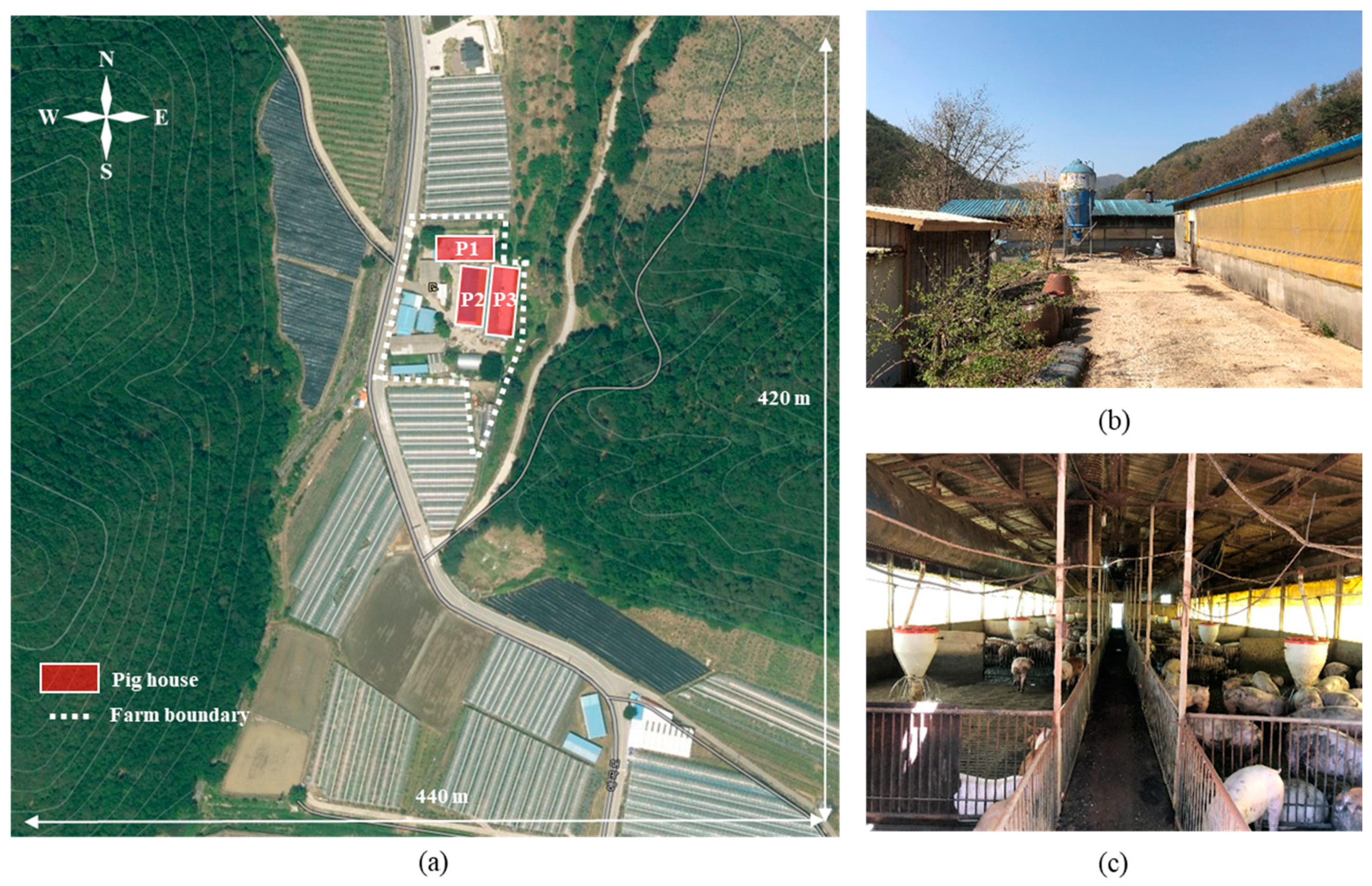
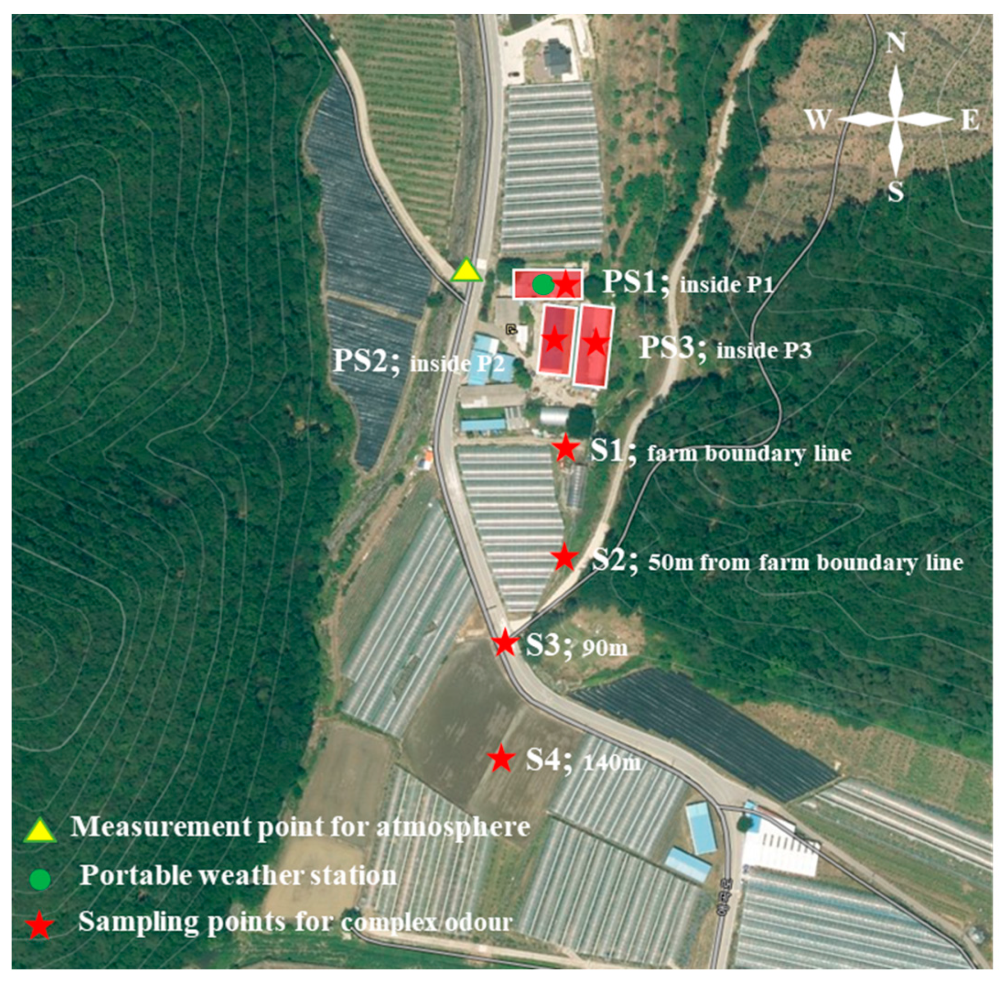
2.1. Farm Description

In the selection of the target experimental farm, it was very important to exclude the interference of livestock odour that was generated from surrounding farms. A commercial pig farm to meet this requirement that was located at Bouen-gun, Chungcheongbukdo, South Korea (127°37′15″ E, 36°28′56″ N) was selected as an experimental farm. The pig farm was located in a valley formed in a north–south orientation. The experimental pig farm consisted of three pig houses, in which, in this study, were referred to as pig house 1 (P1), pig house 2 (P2), and pig house 3 (P3), as shown in Figure 2a. The experimental pig farm raised a total of 850 pigs, with lower than standard rearing density levels of 0.8 m² per finishing pig [52,53]. The farm adopted an all-in and all-out rearing (AIAO) method. P1 has dimensions of 28.0 m in length, 10.0 m in width, and 3.8 m in height. In contrast, P2 and P3, with a perpendicular orientation to P1, have 28.0 m × 13.6 m × 4.5 m and 33.0 m × 10.0 m × 4.3 m in length, width, and height, respectively. All pig houses were equipped with a combined mechanical ventilation and natural ventilation system, consisting of winch curtains and roof-chimney exhaust fans (diameter (D): 0.6 m, 168 cubic meters per minute (CMM)). Roof-chimney exhaust fans were installed at equal intervals in the longitudinal direction of P1 (two fans) and P3 (three fans). On the other hand, considering the relatively wide width of P2, a total of four fans were installed in two rows in the longitudinal direction on the roof of P2. The dimension of the winch curtain for P1 and P2 was 1.0 m × 27.0 m, while the winch curtain for P3 was 1.0 m × 32.0 m. The natural air entered the pig houses through winch curtains that were installed on both sides of each house. The location of the slurry pit was below the pigs and the manure was collected, stored, and removed at the end of every rearing period. The inside and outside conditions of the pig house are shown in Figure 2b,c.

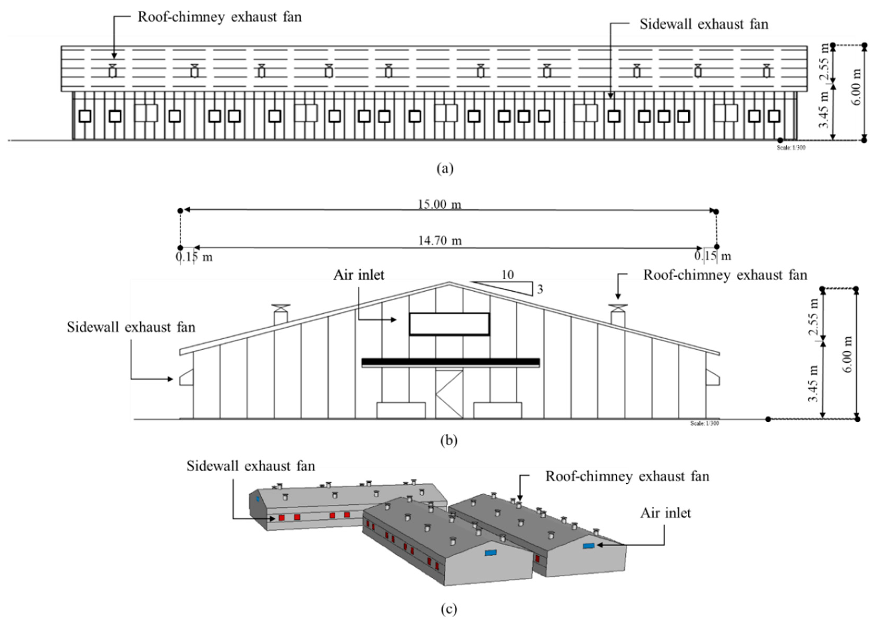
2.2. Korean Standard Pig House

Previously constructed pig houses in the Republic of Korea had been arbitrarily designed depending on the experience of the consultant and allotted budget of the farm owners. This resulted in various structural designs and ventilation systems’ designs of pig houses, causing difficulties in the implementation of technologies to easily maintain a rearing environment, working hygiene, and odour management. Therefore, the Korean government has provided a standard pig house design to be used for constructing new and for renovating old pig houses. This standard design can reduce the economic burden of farm owners at the design stage of the pig house. Moreover, the availability of these standard designs was enormous because government legislation on unauthorized livestock buildings was enacted, and plans were being made for crackdowns and sanctions on the construction of unauthorized livestock buildings. Thus, to represent the approved design of pig houses and common internal and external conditions of a pig house, the CFD model for the case study used the 2016 standard pig house design for the finishing pigs [54].

The schematic diagram of the standard pig house is shown in Figure 3a,b. The length of the Korean standard pig house, including the number and type of exhaust fans, can be modified depending on the farm area, the number of pigs grown, and the farm owner’s preference. Therefore, a fully mechanically ventilated pig house with a similar area as the pig farm in the experimental farm was considered in the computational domain for numerical analysis. The orientation of three standard pig houses followed the same position as the actual experimental pig house. An inlet (1.5 × 0.6 m), which acts as the entrance for fresh air, was also provided on both sides of each structure. Each pig house has 16 sidewall exhaust fans (D: 0.7 m) and 12 roof-chimney exhaust fans (D: 0.5 m). The designed structure of the pig house is shown in Figure 3c.

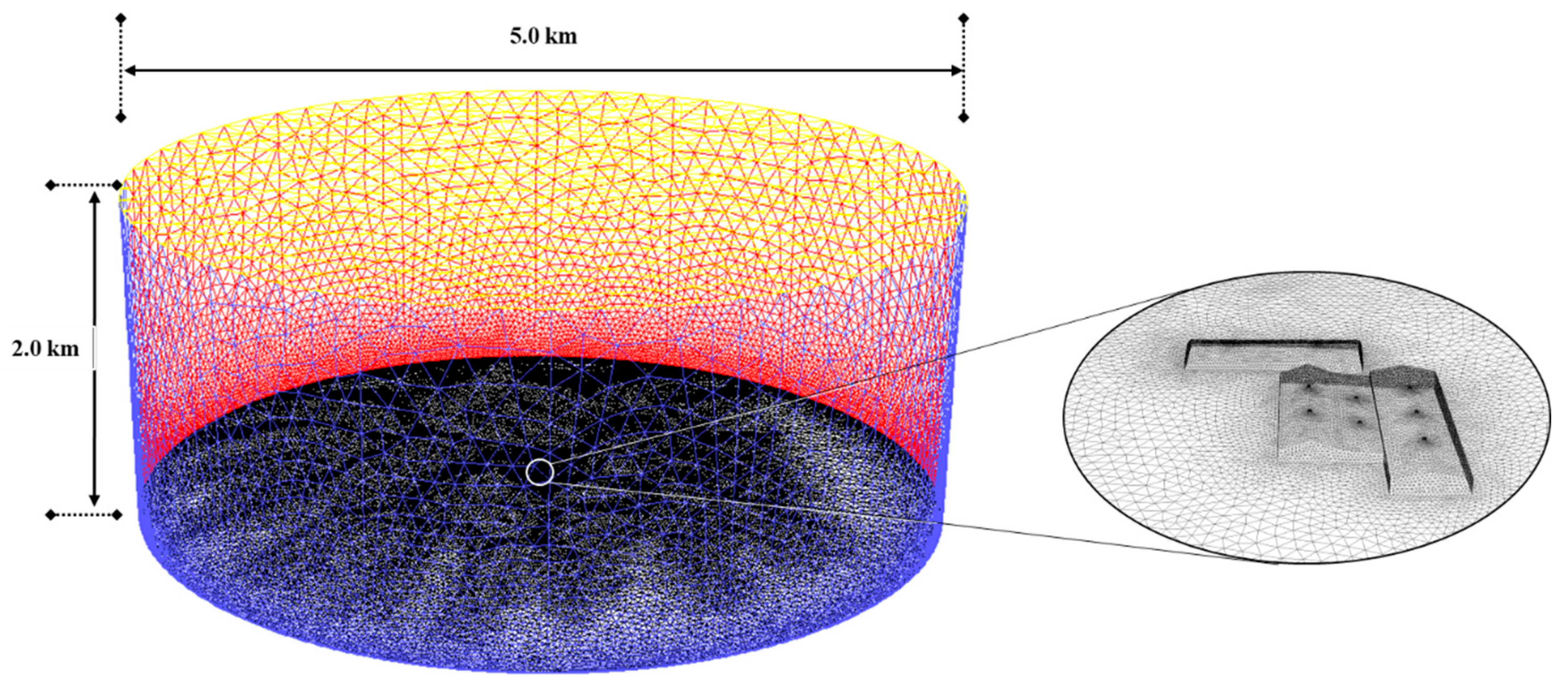
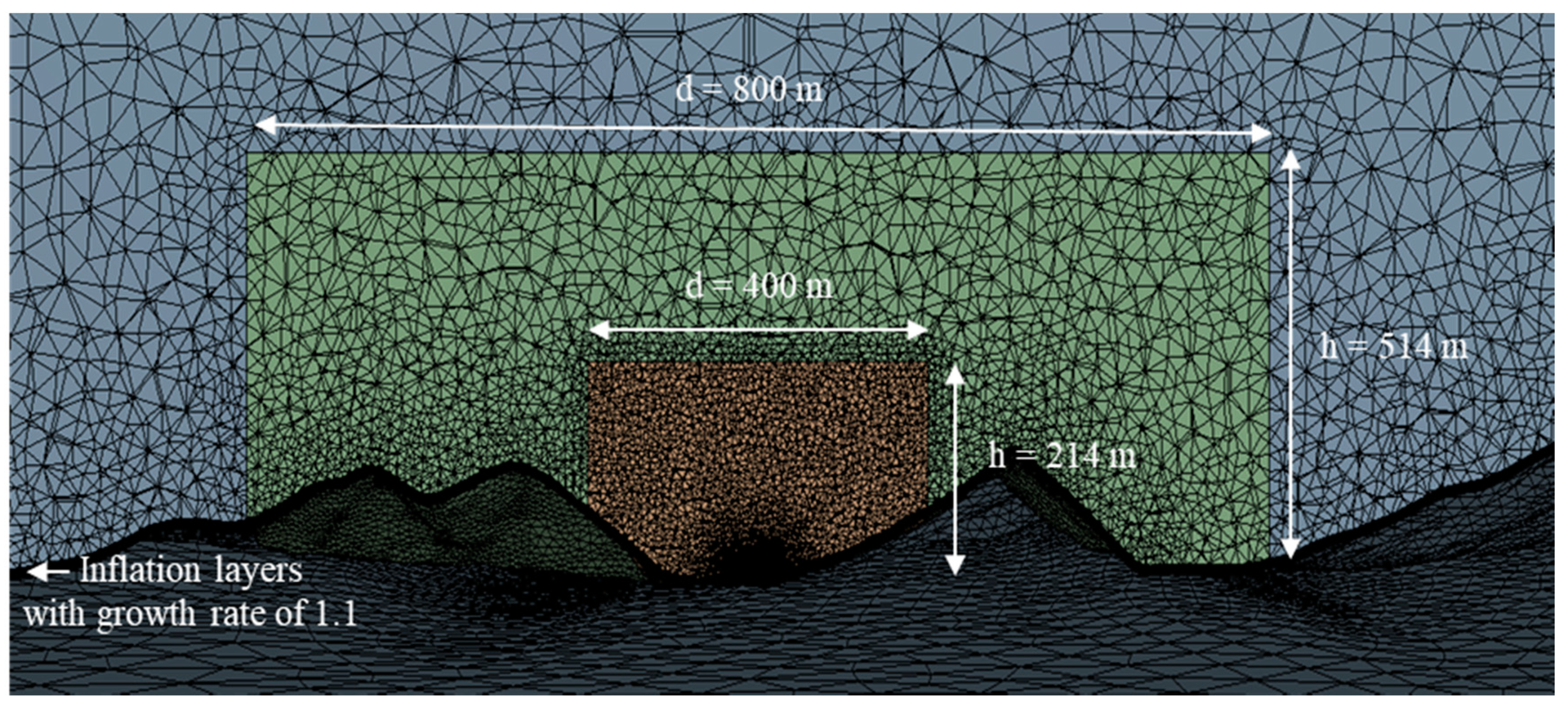
2.3. Design Tool for Numerical Analysis

To accurately evaluate the odour dispersion on a complex terrain like a mountain area, a detailed topographical design should be properly designed before incorporating it into the computational domain [20]. In this study, the complex terrain was developed using commercial software such as ArcGIS, AutoCAD, SketchUp, and Rhino3D. A topographical map of the experimental area, which consisted of contours, elevations, and land use information on the scale of 1:5000 and was obtained from the National Geographic Information Institute (NGII), was used. The ArcMap tool, a software under ArcGIS, was used to edit the digital map. However, when the maps were laid together, borders between the maps were slightly misaligned. Thus, AutoCAD was used to manually modify the contours. It was also used to design the buffer area outside the contour area. The SketchUp tool was used to generate the triangular irregular network (TIN) from the contour lines. Rhino3D, on the other hand, is a modelling tool that can provide great flexibility and precision in handling curves and surfaces. This tool was used to convert the ground from the formed TIN triangulation to solid modelling. The completed ground surface was incorporated in the geometry of the CFD model to analyse the odour dispersion with complex terrain. CFD is a numerical analysis method for predicting phenomena such as fluid flow, heat and mass transfer, and chemical reactions. The governing fluid flow Navier–Stokes equations, which are a set of nonlinear partial differential equations, were formulated in a discretized form through the finite volume method (FVM). Numerical analyses for fluid and energy flow are based on mass, momentum, and energy conservation laws. The conservation equations (Equations (1)–(3)) for each of these physical variables are as follows [55]:

Mass conservation equation:

$$\frac{\partial \rho }{\partial t}+\nabla ·\left(\rho \overrightarrow{\upsilon }\right)=S_m$$

(1)

Energy conservation equation:

$$\frac{\partial }{\partial t}\left(\rho E\right)+\nabla \left(\overrightarrow{\upsilon }\left(\rho E+P_s\right)\right)=\nabla \left(k_{eff}\nabla \mathrm{T}-{\displaystyle \sum }h{\overrightarrow{J}}_i+\left({\overrightarrow{\tau }}_{eff}\overrightarrow{\upsilon }\right)\right)+S_h$$

(2)

Momentum conservation equation:

$$\frac{\partial }{\partial t}\left(\rho \overrightarrow{\upsilon }\right)+\nabla ·\left(\rho \overrightarrow{\upsilon }\overrightarrow{\upsilon }\right)=-\nabla P+\nabla \left(\overrightarrow{\tau }\right)+\rho \overrightarrow{g}+\overrightarrow{F}$$

(3)

where $\rho$ is the density (kg m⁻³), $\overrightarrow{\upsilon }$ is the velocity (m s⁻¹), $S_m$ is a mass source term based on the chemical reaction (kg m⁻²), $E$ is the total energy (kg m² s⁻² kg⁻¹), $P_s$ is the atmospheric pressure (kg m⁻¹ s⁻²), $k_{eff}$ is the effective conductivity (kg m⁻¹ s⁻³ K⁻¹), $\mathrm{T}$ is the temperature (K), $\overrightarrow{\tau }$ is the stress tensor (kg m⁻¹ s⁻²), ${\overrightarrow{\tau }}_{eff}$ is the effective stress tensor (kg m⁻¹ s⁻²), ${\overrightarrow{J}}_i$ is the component of diffusion flux, $S_h$ is the enthalpy rise based on the chemical reaction or radiation (kg m⁻¹ s⁻³), $\overrightarrow{g}$ is the gravitational acceleration (m s⁻²), and $\overrightarrow{F}$ is the external force vector (kg m s⁻²).

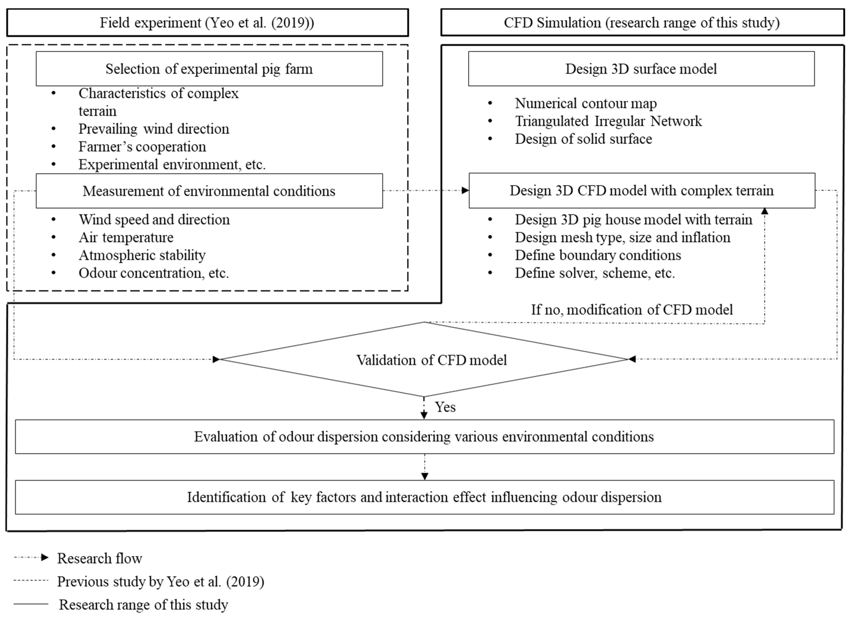
2.4. Description of Experimental Procedures

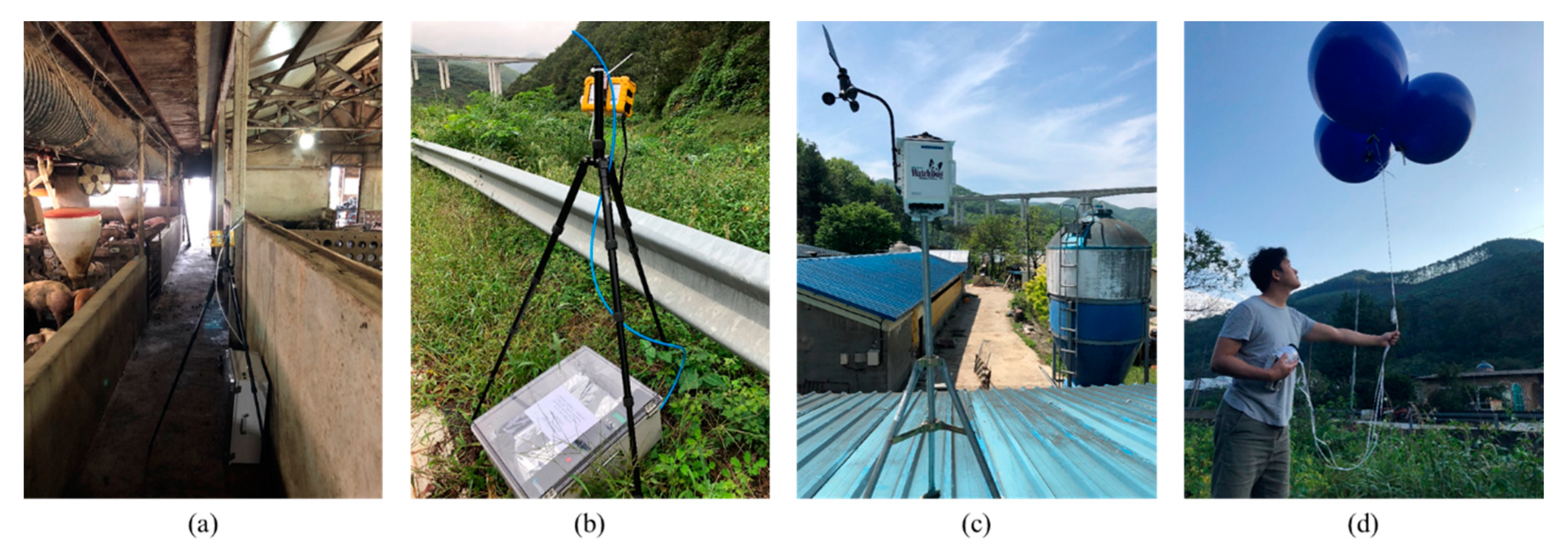
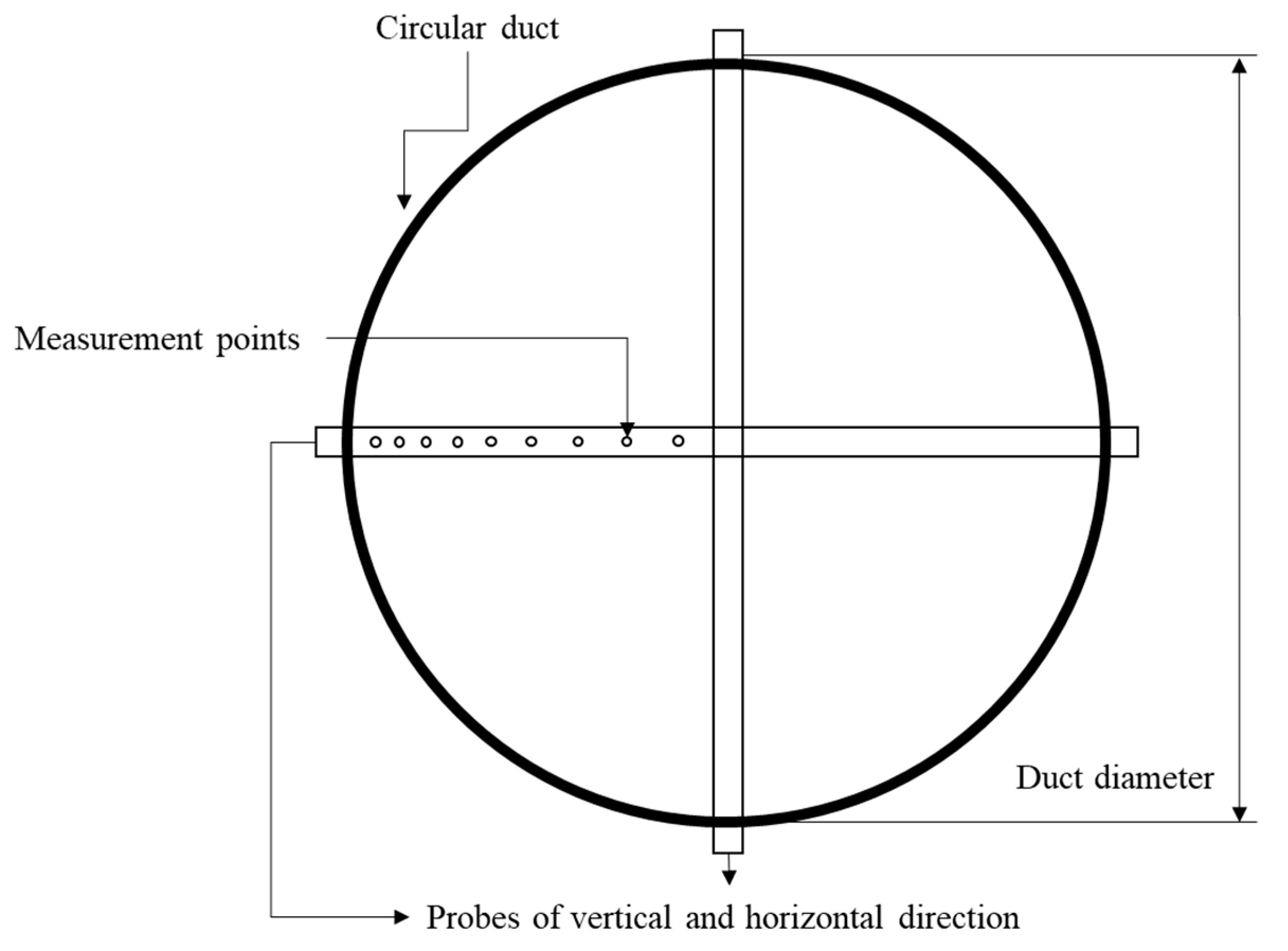
2.4.1. Field Experiment for CFD Model Design and Validation

A data field measurement conducted by Yeo et al. [18] from August 2018 to September 2019 was used to define the initial boundary conditions and validate the designed three-dimensional CFD model. An odour assessment result carried out during four sampling periods was used. The external weather environment that affects odour dispersion and quantitative odour concentration was measured from the field experiment. Shown in Figure 4a,b are the actual setups for collecting odorous air samples inside and outside the pig house facilities. To observe the external weather environment such as wind direction and wind speed, a portable weather station (WatchDog 2700, Spectrum Technologies, Inc., Aurora, IL, USA) was placed at 1.5 m from the roof of P1 with a measuring interval of 1 min (Figure 4c). For on-site atmospheric stability, the vertical distribution of temperature was measured through the hobo sensor (UX100-003, Onset Computer Corp., Bourne, MA, USA) twined on the balloons using a light wire (Figure 4d). The measurement location of the atmospheric stability was set up to a place so that it was free from any obstacles around the experimental pig house. The atmospheric stability was measured at 1-min intervals. Odour generated from pig houses was also measured to determine the odour concentration dispersed at a certain distance at specific atmospheric stability. The measured odour concentration was used to validate the CFD model. Odour samples at different sampling locations were collected simultaneously using a portable air sampler (Odortech, Seoul, Korea). The actual setup of field instruments is illustrated in Figure 4. The sampling locations for the field measurement of odour concentration were inside the pig houses and outside the pig houses. All measuring devices were located 1.5 m high from the ground surface. For inside the pig house, sampling instruments were installed near the location of the outlet. The sampling location outside the pig houses was established at 40.0 to 50.0 m intervals from the farm’s boundary line. Sampling locations inside the pig houses were designated as PS1, PS2, and PS3 depending on the pig house, while in the case of sampling points outside, S1, S2, S3, and S4 were used (Figure 5).

Following the field experiment, a sensory evaluation was conducted to determine the concentration of odour obtained from various sampling points. The test method followed the air dilution sensory guidelines of the odour process test (ES 09301.a) [53,54]. The collected air samples were transported to the laboratory for sensory evaluation within 24 h and were kept at room temperature (15 to 25 °C) to maintain the quality of samples obtained from the field. The odourless air was made from the clean air generator (Anytech Inc., Suwon, Korea). This device contained silica gel and activated carbon to eliminate moisture and odour. The diluted air samples were made by mixing odorous and odourless air in consideration of the dilution rate, by injecting the odorous air sample into Tedlar bags with clean air samples. The diluted air samples were distributed to the panels through a 5-p distributor (Anytech Inc., Suwon, Korea). When conducting the evaluation, the same panels were employed during the experiment period to eliminate the uncertainty in the odour concentration caused by employing different panels. Each set comprised three air samples, where one sample contained odour and two with only odourless air. The sensory evaluation followed the “triangular-forced-choice” process, where panellists sniff all three samples and must select which among the three samples contain the diluted odour. The odour concentration based on the evaluation results performed by five panellists, excluding the maximum and minimum values to prevent from being overestimated or underestimated, was calculated using the geometric mean [53].

2.4.2. Design, Validation, and Case Study Using the CFD Model

A three-dimensional CFD model for the simulation of livestock odour dispersion is shown in Figure 6; it has an area of 5.0 km in diameter, including 2 km of the buffer area, and 2.0 km in height. Because the odour dispersion problem is mainly generated in the lower part of the atmospheric layer, and the height of the grid located near the ground surfaces large, it is difficult to simulate the rapid wind speed change near the ground. Therefore, the domain was discretized by a non-structural grid strategy. This means that the size and density of grids used in the domain were not uniform. Purposely, the grid near the pig houses and the ground was designed denser and became coarser with the increase in altitude. This kind of grid generation approach ensures a high degree of grid precision in the area close to the odour sources [45]. To precisely compute odour concentration near the surface, the CFD model was designed by using the inflation function. The first layer height used 0.1 m at the ground surface, and 25 layers with a growth rate of 1.1. To validate the CFD model, a standard design of a pig house model was placed in the centre of the computational domain, as shown in Figure 6. A grid size of 0.2 m around the roof-chimney exhaust fan of the pig house was used to design a grid where the odour was mainly emitted. Other than the roof-chimney exhaust fan, 0.5 m of grid size was used around the wall of the pig house. Additionally, to calculate more accurate airflow and odour distribution around the pig house, the grid was designed with a size of 2.0 m in the 200.0 m radius around the pig house. After 200.0 m, the CFD model was designed with a growth rate of 1.1 to reduce the total number of grids, while gradually increasing the grid size (Figure 7). In the same way, the CFD model (the 2016 standard pig house design) for the case study applied all the grid design methods used in the design of the validation model.

The proper design for the grid size is an important factor that can influence not only the computational time but also the accuracy and reliability of the results. The smaller the grid size, the more detailed and accurate the numerical value can be calculated. However, the computation time increases as the number of grids increases, which may not be efficient. Therefore, it is necessary to conduct the grid independence test, which selects a reasonable grid size by designing grids of various sizes in the calculation domain and comparing them with field-measured data. This takes into account the computational characteristics that the grid results no longer change significantly as the grid size becomes smaller and denser. In this study, the grid sizes from the outside of the pig house to the buffer space in the calculation domain were fixed to 4.0, 10.0, 20.0, and 40.0 m, except for the inlet, outlet, and ground surface, which requires the design of a small grid in the flow analysis, and was compared with field experiments.

Similarly, the selection of an appropriate time step to be used in the validation is an important factor that influenced the accuracy and economics of the simulation procedure. In general, the smaller the size of the calculation time step, the better the ability to simulate certain phenomena. In this study, the time steps of 1, 5, 10, and 20 s were considered for a calculation time of 10 min.

In analysing the flow of air, the choice of turbulence model is important because the turbulence characteristics may vary according to the turbulence model selected in the computational domain. Turbulent flow is a type of flow that undergoes irregular fluctuation or mixing. Turbulent flow has a smaller dispersion compared to laminar flow with a low Reynolds number, convection acts largely in a certain space, and pressure and velocity change rapidly over time and space. Therefore, tests on turbulence models, which are widely applied in the field of flow analysis in agricultural facilities, were conducted. In the same way as the grid independence test, an appropriate turbulence model to be able to improve the accuracy of the CFD-computed results was determined by comparing the field-measured data with the CFD-computed results with R² (R-square) and RMSE (root mean square error). The tested turbulence models include RANS (Reynolds-averaged Navier–Stokes) models (standard k-epsilon model, renormalized group (RNG) k-epsilon model, realizable k-epsilon model) and the Large Eddy Simulation (LES) model. The RANS model is time-averaged equations of motion for fluid flow. RANS models would weaken and be replaced by large eddy simulation (LES) as a consequence of rapidly increasing computational power. Certainly, greater reliance on the unaveraged Navier–Stokes equations means more accurate results. The k-epsilon (k-ε) turbulence model for the RANS model is the most common model used in CFD to simulate mean flow characteristics for turbulent flow conditions. Among the k-epsilon turbulence models, there are differences in the turbulent viscosity and transport equation for turbulent dissipation. Therefore, the effort of selecting a suitable turbulence model from the k-epsilon and LES models for turbulence analysis was made. Statistical indices, such as R² and RSME, were used to determine the grid sizes and turbulent models were appropriate to be used in this study.

The stability or instability of the atmosphere is a condition that considers the reaction of a volume of an air parcel to vertical displacement. The stability of the atmosphere determines the probability of convective activity, cloud type, atmospheric turbulence, and degree of vertical mixing (for pollutants, etc.). The classification of atmospheric stability includes stable, neutral, and unstable conditions. Atmospheric stability is related to the wind profile expressed as Equation (4). Specifically, the wind profile was based on a log wind profile which is used to describe the vertical wind characteristics.

$$\frac{\mathrm{kz}}{{\mathrm{u}}^{\ast }} \frac{\partial \mathrm{u}}{\partial \mathrm{z}}{= \Phi }_{\mathrm{m}}$$

(4)

where k is the von Karman constant (0.42); z is the altitude above ground; u* is the friction velocity; u is the velocity magnitude; Φ_m is the Monin–Obukhov universal function for non-dimensional momentum.

To express the Monin–Obukhov universal function for the stable atmospheric stability in this study, the equations (Equations (5)–(7)) were adopted from the empirical equation created by Dryer and Hicks [56] and Hicks [57] as cited by Hong et al. [20]. The Φ_m was expressed using the following equations:

$${\Phi }_{\mathrm{m}}= 1: \mathrm{neutral}$$

(5)

$${\Phi }_{\mathrm{m}}=1+\frac{5\mathrm{z}}{\mathrm{L}}: \mathrm{stable}$$

(6)

$${\Phi }_{\mathrm{m}}={\left(1-\frac{16\mathrm{z}}{\mathrm{L}}\right)}^{-0.25}: \mathrm{unstable}$$

(7)

where L is the Obukhov length and z is the height from the surface.

The assumption in the Monin–Obukhov similarity theory was adopted that when the calculated value of the Monin–Obukhov universal function has a value of infinity and almost equal to 1, the atmospheric stability is neutral. Similarly, stable air happens when the surface absorbs heat and the Obukhov length (L) is positive. Conversely, the unstable air condition occurs when the Obukhov length (L) is negative. Therefore, by integration, the following equations used to describe the vertical wind profile were expressed as Equations (8)–(10):

$$\mathrm{U}\left(\mathrm{z}\right)=\frac{{\mathrm{u}}_{\ast }}{\mathrm{k}}\left[\ln \left(\frac{\mathrm{z}}{{\mathrm{z}}_0}\right)\right]: \mathrm{neutral}$$

(8)

$$\mathrm{U}\left(\mathrm{z}\right)=\frac{{\mathrm{u}}_{\ast }}{\mathrm{k}}\left[\ln \left(\frac{\mathrm{z}}{{\mathrm{z}}_0}\right)+5\frac{\mathrm{z}}{\mathrm{L}}\right]: \mathrm{stable}$$

(9)

$$\mathrm{U}\left(\mathrm{z}\right)=\frac{{\mathrm{u}}_{\ast }}{\mathrm{k}}\left[\ln \left(\frac{\mathrm{z}}{{\mathrm{z}}_0}\right)-2\ln \left(\frac{1+\mathrm{x}}{2}\right)-\ln \left(\frac{{1+\mathrm{x}}^2}{2}\right){+2\tan }^{-1}\left(\mathrm{x}\right)-\frac{\mathsf{\pi }}{2}\right]: \mathrm{unstable}$$

(10)

where $\mathrm{U}\left(\mathrm{z}\right)$ is the magnitude of the mean horizontal velocity at the height z (z > ${\mathrm{z}}_0$); u* is the friction velocity; k is the von Karman constant; z is the height from the surface; ${\mathrm{z}}_0$ is the roughness length of the surface; L is the Obukhov length; x is the dimensionless variable defined by the equation used to describe the Monin–Obukhov universal function.

Several qualitative and quantitative measures have been conducted by many researchers to create an air temperature profile. In this study, the dry adiabatic lapse rate for microclimate conditions cited by Bache and Johnstone [58] was adopted to present the temperature turbulence or the change in temperature according to height. For a neutral atmosphere, the temperature cools down by 1 °C for every 100 m increase in height (−0.01 °C m⁻¹). Meanwhile, a lapse rate of 0.015 and −0.02 °C⁻¹ was used for stable and unstable conditions, respectively.

Table 1. Constant input values for the case file of the CFD models.

Main Parameter		Input Values
		Model for Validation *	Model for Case Study **
			Sidewall Exhaust Fan	Roof-Chimney Exhaust Fan	Sidewall + Roof-Chimney Exhaust Fan
Wind speed of fans	P1	8.94 m s−1	6.8 m s−1	11.59 m s−1	5.5 m s−1 (sidewall) 5.37 m s−1 (roof-chimney)
	P2	3.84 m s−1, 7.08 m s−1
	P3	6.38 m s−1
Odour concentration	P1	100 OU m−3	577.5 OU m−3
	P2	64.3 OU m−3
	P3	448 OU m−3
Wind Speed		0.5 m s−1	0.5, 1.5, 2.5 m s−1
Atmospheric stability		stable	stable, neutral, unstable
Convergence criteria		$1\times {10}^{-6}$
Temperature		299.45 K
Density of air		1.225 kg m−3
Gravitational acceleration of air		9.81 m s−2
Atmospheric pressure		101,325 Pa
Wind speed		0.5, 1.5, 2.5 m s−1
Grid size		selected from the grid independence test (4.0, 10.0, 20.0, and 40.0 m)
Time step		selected from the time step test (1, 5, 10, 20 s)
Turbulence models		selected from the validation test (Standard k–ε, RNG k–ε, Realisable k–ε, LES)

* field measured data; ** computed data.

shows the initial boundary conditions of the model for CFD simulation. The speed of the exhaust fan of the CFD model for validation was applied by measuring the wind speed of the fan at nine points when the exhaust fan ran at maximum (Figure 8). To measure the air flow rate of a circular exhaust fan, a traverse method was applied at the duct surface using hot wire anemometers to measure the discharged speed. The measurement points (9 points) were selected based on ASHRAE (American Society of Heating, Refrigerating and Air-Conditioning Engineers) standards [59].

While the wind speed of the exhaust fan for the case study was analysed by applying the ventilation flow rate provided by the manufacturer to the CFD model, in the case of the Korean standard pig house used for the case study, ventilation rates of the pig house were calculated from the ventilation requirement per pig in the summer season presented in the Midwest Plan Service (MWPS) for finishing pigs during the summer season. The summer season was preferred in this study, since odour dispersion was very dynamic during this season due to high air temperature and active microbial activities. The wind speeds of 6.8 and 11.6 m s⁻¹ were applied to the sidewall and roof-chimney exhaust fan, respectively. Similarly, in the case of odour concentration generated in each pig house, the validation model applied the same odour value measured in the field. For the case study, the odour emissions from each pig house were calculated using emission factors established by Belgium [60]. The generation of odour for pigs in summer was defined as 32.7 OU animal⁻¹ s⁻¹. Considering the number of pigs per unit area, the total odour unit was 40,188.3 OU s⁻¹. The total odour concentration needs to be converted into a mass fraction value using the Equation (11) described in Hong et al. (2011):

$$Y_s=\frac{{\mathrm{O}}_{\mathrm{cg}}{\times \mathrm{m}}_{\mathrm{c}}}{\frac{{\mathrm{P}}_{\mathrm{a}}\mathrm{M}}{\mathrm{RT}}{+ \mathrm{O}}_{\mathrm{cg}}{\times \mathrm{m}}_{\mathrm{c}}}$$

(11)

where $Y_s$ is the odour mass fraction; P_a is the atmospheric pressure of 101,325 Pa at sea level; T the air temperature in K; M the molecular weight of dry air or 0.028966 kg s⁻¹; R is the universal gas constant of 8.31432 J (mol·K)⁻¹; O_cg the odour source concentration in OU m⁻³; m_c the mass of odour compound (n-butanol) required to produce one odour unit.

For the computation of the CFD model, a pressure-based solver, which is widely applicable in flow analysis, was performed and the gravitational acceleration was set to −9.81 m s⁻². A standard operating pressure of 101,325 Pa was applied. The solution was assumed to have converged when the sum of residuals for all of the cells in the computational domain was less than $1\times {10}^{-6}$ for continuity and energy, and $1\times {10}^{-3}$ for other variables such as X, Y, Z-velocity, k, and ε.

As mentioned, odour dispersion in the atmosphere may vary depending on weather and structural variables. Therefore, wind speed (0.5, 1.5, and 2.5 m s⁻¹), wind direction (north, east, south, and west), and atmospheric stability (stable, neutral, and unstable) were considered as weather factors, while the roof-chimney exhaust fan, sidewall exhaust fan, and conditions for using all the exhaust fans were considered as structural factors. The case study using 108 simulation cases for the standard Korean pig house was conducted using the determined grid size and turbulence model to evaluate the effect of various factors on odour dispersion distance. Data were calculated and analysed at the level of 1 OU, the minimum level of odour that humans could recognize at 1.5 m from the ground level.

2.5. Statistical Analysis for Identifying Key Factors Influencing Odour Dispersion

For the case study results, statistical analyses were conducted using the Statistical Package for the Social Sciences (SPSS) program (ver. 23.0, IBM Inc., Armonk, NY, USA). From the CFD-computed odour dispersion distances, a statistical analysis was performed to determine the key factors influencing odour dispersion distance. Before the analysis, a multicollinearity test was first carried out to determine which among the selected factors would be included in the multiple regression analysis. Multicollinearity between variables can cause a problem because it can increase the variance of the coefficient estimates and make the estimates very sensitive to minor changes in the model. A common criterion for multicollinearity problems includes calculation of the tolerance and variance inflation factor (VIF), as shown in Equations (12) and (13). Tolerance is associated with each independent variable and ranges from 0 to 1, while VIF with a value exceeding 10 is often regarded as indicating multicollinearity. Accordingly, when high multicollinearity was found, a highly correlated independent variable from the model was removed.

$$\mathrm{Tolerance} = 1-{\mathrm{R}}_{\mathrm{i}}^2$$

(12)

$$\mathrm{VIF}= \frac{1}{{1-\mathrm{R}}_{\mathrm{i}}^2}$$

(13)

where ${\mathrm{R}}_{\mathrm{i}}^2$ is the coefficient of determination between i-th independent variable and other independent variables, and VIF is the reciprocal of tolerance and quantifies the severity of multicollinearity in an ordinary least squares regression analysis.

Multiple regression analysis is a statistical approach used to predict the value of the dependent variable based on the value of two or more independent variables. This tool shows how the variation of each factor influences the total value of the predicted result. Using this analysis, the relative influences of the considered independent variable can be analysed. To supplement the result of the regression analysis, the statistical method called the relative weight analysis (RWA) method was implemented to identify which among the independent variables had the greatest contribution to odour dispersion. The RWA method is a tool that addresses the multicollinearity problem and helped to calculate the relative importance of an independent variable. In this method, the variables transformation approach was carried out to create a new set of predictors that are orthogonal to one another. The general procedure determining the RWA was to create and describe the relationship between the original variables and the orthogonal variables through the regression equation. Relative weight can be calculated using the following equations (Equations (14) and (15)) based on the procedure established by Tonidandel et al. [61]:

$${\mathrm{R}}^2= 1-\frac{{\displaystyle \sum }{\left(y_i- {\widehat{y}}_i\right)}^2}{{\displaystyle \sum }{\left(y_i- {\overline{y}}_{ }\right)}^2}= {\displaystyle \sum }\mathrm{Raw} \mathrm{Relative} \mathrm{weights}$$

(14)

$$\mathrm{Relative} \mathrm{Weight} = \left(\frac{\mathrm{Raw} \mathrm{relative} \mathrm{weight}}{{\mathrm{R}}_{ }^2}\right)\times 100$$

(15)

where R² is the coefficient of determination; y_i is the y value for observation i; ${\widehat{y}}_i$ is the predicted value of y for observation i; $\overline{y}$ is the mean of y value.

3. Results

3.1. Field Experiment Results (Yeo et al., 2019)

Since the dispersion of odour in the surrounding area was greatly influenced by environmental factors, field measurement of various meteorological conditions such as wind speed and the temperature was first conducted. The prevailing wind was northerly winds based on analysis from a weather station near the farm (analysis period: 1997.1.1–2017.12.31). This result was similar to a portable weather station installed in the experimental pig house. The result of the prevailing wind direction was greatly influenced by the topographical location of the pig houses as the selected farm was surrounded by hills along the eastern and western parts. This type of topographical orientation reduced the impact of wind originating from the east and west part of the computational domain. The atmospheric stability during the conduct of the field experiment was generally stable with a temperature ranging from 15.7 to 33.5 °C and wind was 0.5 m s⁻¹, as shown in

Table 2. Odour concentration at various sampling points [18].

Date	Air Temperature (°C)	Odour Concentration (OU m−3)
		PS1	PS2	PS3	S1	S2	S3	S4
8 August * (a.m.)	26.3	44.8	5.5	20.8	4.6	2.1	1.4	3.0
8 August * (p.m.)	33.5	11.8	5.5	5.5	2.1	1.0	1.4	3.1
6 September * (a.m.)	15.7	311.0	44.8	30.0	1.7	3.1	2.1	1.4
6 September * (p.m.)	26.2	448.1	100	64.6	6.7	2.5	1.4	1.2

* Atmospheric stability: stable; wind speed: 0.5 m s⁻¹; wind direction: north.

. In terms of odour concentration measured, a detailed summary can be found in the study of Yeo et al. [18]. The amount of odour concentration inside the pig house had higher concentration during September, with a value ranging from 30.0 to 448.1 OU m⁻³ compared to August, with values ranging only from 5.5 to 44.8 OU m⁻³. The variation in measured odour concentration inside the pig house was due to the large volume of manure present in the slurry pit during September. During this month, the farm owner no longer disposes of the manure, since the rearing period for that season was almost due. The amount of odour concentration measured outside the pig house was significantly lower compared to inside the pig house. This result accounted for the dilution of concentrated odour with clean air outside the pig house when the inside odour comes out from the pig house facilities. Considering that the amount of odour concentrations measured inside the pig houses was highest at the end of the rearing period, and a distinct odour concentration trend downwind of the pig houses was found, the field-measured odour concentration on September 6 was therefore used as a reference value to validate the CFD model by comparing the CFD-computed results and the field-measured data. Moreover, the field experiment result showed that the measured odour concentration at the boundary of the pig farm falls below the minimum level of allowable OU m⁻³ value set by the Korean government, which was 15 OU m⁻³. This means that the odour emission complied with the maximum OU m⁻³ limit for Korean livestock houses.

3.2. Validation of the CFD Simulation Model

The validation of the designed CFD model included the grid independence test, time step test, and turbulence test. The size of the grids must be well identified, since it contributed to the accuracy of the CFD-computed results. Since the size of the computational domain has a large diameter of 5.0 km, the grid independence test of the CFD model was carried out using four grid sizes (4.0, 10.0, 20.0, and 40.0 m). According to the designed grid, the number of grids in the computational domain ranged from 3.76 million to 8.73 million combined hexahedral and tetrahedral elements. The number of grid elements decreased when a larger grid size was used, whereas a greater number of grid elements were created when smaller grids sizes were used. After convergence was achieved, the CFD-computed results showed considerable differences in the predicted odour between the four grid sizes as summarized in

Table 3. CFD-computed odour concentration at various sampling locations according to grid size.

Grid Size	Number of Elements (Million)	Odour Concentration (OU m−3)
		S1	S2	S3	S4	R2	RMSE
Field experiment	-	6.7	2.5	1.4	1.2	-	-
4.0 m	8.73	7.40	1.75	0.04	0.00	0.999	1.06
10.0 m	5.16	6.79	1.33	0.03	0.00	0.998	1.09
20.0 m	3.98	14.97	2.00	0.09	0.00	0.991	4.24
40.0 m	3.76	9.79	1.68	0.09	0.00	0.996	1.84

. When the RMSE was analysed, the model which designed the grid with a size of 4.0 m had the lowest error, while the error was significant when the grid was larger than 10.0 m. The CFD model, which had a relatively large grid size, such as 20.0 and 40.0 m, showed imprecise odour concentration results when compared with the field-measured data, while both the 4.0 and 10.0 m grids calculated the odour concentration relatively close to the field-measured data. These grid sizes obtained the highest R² value of 0.999 and 0.998 and lowest RSME value of 1.06 and 1.09, respectively. However, for the grid sizes of 4.0 and 10.0 m, there was no significant difference between the CFD-computed results and the field-measured data. Therefore, considering efficient computation time, the grid size for the CFD model was determined to be 10.0 m.

The simulation results according to the four time steps are shown in

Table 4. CFD-computed odour concentration at various sampling locations according to time step.

Time Step	Odour Concentration (OU m−3)
	S1	S2	S3	S4	R2	RMSE
Field experiment	6.7	2.5	1.4	1.2	-	-
1 s	7.69	1.40	0.20	0.23	0.994	1.083
5 s	6.79	1.33	0.03	0.00	0.998	1.093
10 s	16.56	1.96	0.04	0.01	0.988	5.027
20 s	25.99	1.31	0.04	0.02	0.969	9.711

. The use of 10- and 20-s time intervals confirmed that the RSME (5.027 and 9.711) were relatively large compared to smaller time steps. In contrast, almost identical results were obtained between 1 and 5 s, with an RMSE level of 1.083 and 1.093, respectively. Based on this, it can be concluded that the accuracy of the simulation results using the simulation model is inversely proportional to the size of the time step. Considering the excessive calculation time when using the 1 s time step, the 5 s time step was selected as the most economic time step value to be used in the simulation.

The results related to the turbulence model are summarized in

Table 5. CFD-computed odour concentration at sampling locations according to the turbulence model.

	Odour Concentration (OU m−3)
	S1	S2	S3	S4	R2	RMSE
Measured	6.7	2.5	1.4	1.2	-	-
Standard k-ε	6.79	1.33	0.03	0.00	0.998	1.09
RNG k-ε	7.26	0.54	0.00	0.00	0.977	1.39
Standard k-ω	5.18	0.11	0.00	0.00	0.960	1.70
LES	3.49	0.26	0.00	0.00	0.977	2.17

. Considering the different turbulence models commonly used in odour dispersion studies, in this research, a total of four turbulence models were tested including the standard k-ε model, the RNG k-ε model, the standard k-ω model, and the LES model. The comparison of four turbulence models showed lower RMSE values for the standard k-ε and the RNG k-ε models. Statistical analysis with lower RSME values meant that the CFD-computed results had some discrepancy with the field-measured data. The results showed that the CFD-computed results using the standard k-ε model have the lowest RSME value of 1.093 compared with the other three models, with RSME values of 1.385, 1.696, and 2.165 for the RNG k-ε, standard k-ω, and LES models, respectively. Considering the statistical analysis results, the standard k-ε model was found to be the most appropriate turbulence model to be used.

3.3. Case Study of Odour Dispersion

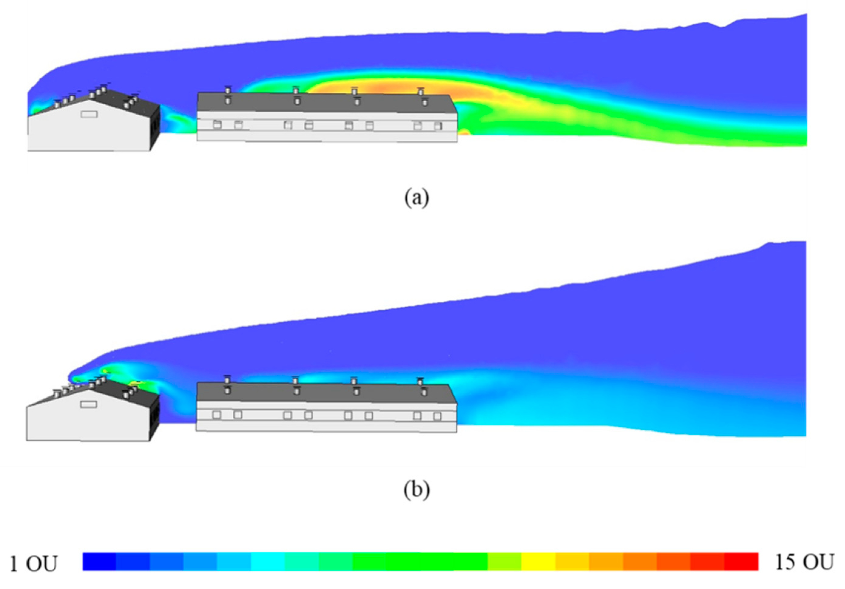
3.3.1. Effect of Ventilation Types on Odour Dispersion

The odour dispersion distance when the sidewall exhaust fan or roof-chimney exhaust fan was used in the pig house was calculated using CFD. The CFD-computed results for the odour dispersion distance are summarized in

Table 6. CFD-computed odour dispersion distance according to various factors.

Ventilation Type	Speed	Atmospheric Condition	Dispersion Distance (m)
			Northerly Wind	Easterly Wind	Southerly Wind	Westerly Wind
Sidewall exhaust	0.5 m s−1	Stable	1081.3	541.3	1427.4	567.7
		Neutral	782.9	401.7	1488.1	478.0
		Unstable	349.6	346.0	485.3	304.3
	1.5 m s−1	Stable	640.4	213.6	653.4	332.7
		Neutral	470.7	213.4	564.8	277.4
		Unstable	230.4	168.3	231.7	182.9
	2.5 m s−1	Stable	479.6	186.7	573.5	256.9
		Neutral	273.3	153.6	491.8	301.8
		Unstable	182.1	147.8	186.4	151.9
Roof-chimney exhaust	0.5 m s−1	Stable	595.1	207.2	817.6	352.4
		Neutral	651.2	293.7	900.6	295.9
		Unstable	224.0	154.9	235.2	220.6
	1.5 m s−1	Stable	256.2	144.4	309.9	148.4
		Neutral	267.9	149.0	304.2	218.9
		Unstable	169.8	107.8	165.3	118.2
	2.5 m s−1	Stable	221.5	130.7	227.6	112.3
		Neutral	151.7	106.7	230.6	120.6
		Unstable	129.7	91.0	114.4	78.9
Sidewall + Roof-chimney exhaust	0.5 m s−1	Stable	579.4	300.5	652.2	392.9
		Neutral	614.4	311.7	928.2	410.0
		Unstable	293.0	194.4	318.3	210.7
	1.5 m s−1	Stable	256.1	146.6	323.2	157.5
		Neutral	255.7	151.6	309.9	164.6
		Unstable	178.4	110.1	168.4	142.9
	2.5 m s−1	Stable	228.5	136.8	238.0	126.5
		Neutral	256.7	138.2	239.5	131.1
		Unstable	142.4	94.0	117.6	92.0

. The CFD-computed results according to the cases ranged from a minimum of 78.9 m to a maximum of 1488.1 m. When using a sidewall exhaust fan, the odour dispersion ranged from 147.8 to 1488.1 m, depending on the case being simulated. On the other hand, the roof-chimney exhaust fan showed a minimum of 78.9 m to a maximum dispersion distance of 900.6 m. On average, the odour dispersion distance was 439.4 m when the exhaust fan on the sidewall was used, while the odour dispersion distance was 250.7 m when the roof-chimney exhaust fan was used. Specifically, the highest dispersion distance was computed when the atmospheric stability was neutral, the wind speed was low, the southerly wind was used, and the sidewall exhaust fan was operated. The lowest odour dispersion distance was computed when the atmospheric stability was unstable, the wind speed was high, with a westerly wind, and the roof-chimney exhaust fan was used. Under the same environmental conditions, there was a difference of 41.3% (maximum: 61.7%, minimum: 16.8%) dispersion distance, depending on the physical environment (ventilation method; sidewall exhaust fan; roof-chimney exhaust fan). The trend of odour dispersing outside the pig house according to the ventilation method under the condition of the north wind direction, wind speed of 1.5 m s⁻¹, and stable condition in the atmospheric stability is shown in Figure 9. Given that the initial amount of odour emission from exhaust fans is almost identical between the ventilation systems (577.5 OU m⁻³), it can be seen that the odour concentration emitted from the pig house using the sidewall exhaust fans was higher near the surrounding area of the pig houses. On the other hand, when the roof-chimney exhaust fan was used, the odour discharged through the exhaust fan has a lower odour concentration. Moreover, when the sidewall exhaust fan and the chimney exhaust fan were used simultaneously, the spreading distance of odour outside the pig house was 92.0 to 928.2 m depending on wind speed, wind direction, and atmospheric stability conditions. The odour dispersion distance was estimated to be 5.4% higher than that of the exhaust using only the roof-chimney exhaust fan. The emission of odour at the sidewall exhaust fan contributed to the increase in the distribution of the odour along downwind.

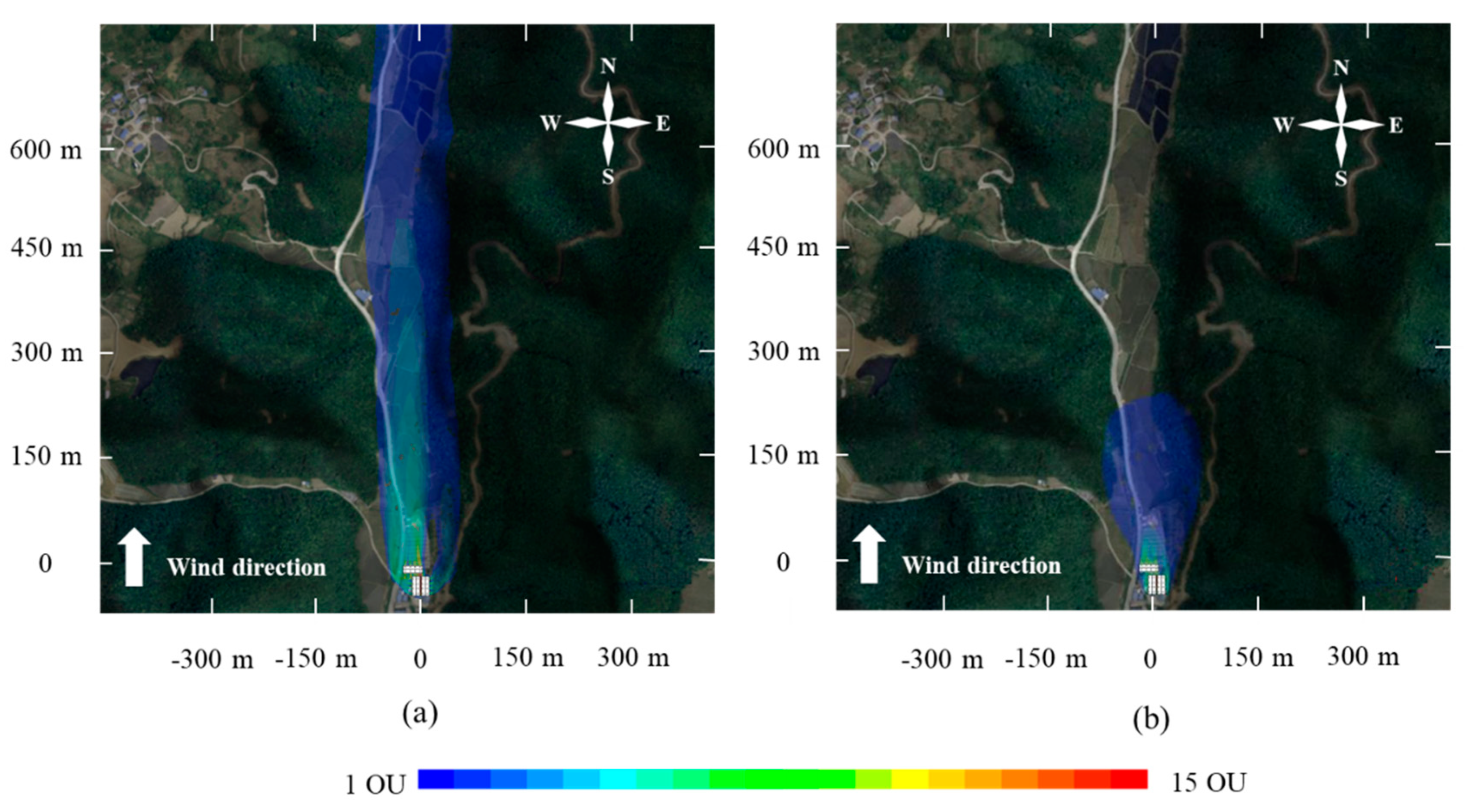
3.3.2. Effect of Atmospheric Stability in Odour Dispersion

The condition of the atmosphere is an important factor in determining the dispersion of odour in the atmosphere. The dispersion distance of odour emitted from pig houses when the condition of the atmosphere was stable was calculated from 112.3 to 1427.4 m. The average dispersion distance was 389.3 m. On the other hand, when the atmospheric stability was unstable, the odour emitted from the pig houses dispersed at a maximum distance of 485.3 m, a minimum of 78.9 m, and an average of 190.0 m. It decreased by 51.3% on average due to the change in atmospheric stability (stable to unstable). This was because, when the atmosphere was stable, the influence of the vertical momentum of air was relatively small resulting in higher odour dispersion distance. However, even if the atmospheric stability was stable, the dispersion distance of the odour was not extended. It was confirmed that the dispersion distance was greatly affected by the presence or absence of the obstacles toward the direction of the wind and wind speed. In contrast, when the atmospheric stability was unstable, vertical mixing and dispersion were very active, so the odour concentration was low near the ground, and the dispersion distance was short as well (Figure 10). In addition, there was no significant difference between stable and neutral conditions in the stability of the atmosphere. The same trend result was found in the odour dispersion modelling result [20,45,60]. Representative figures showing odour dispersion according to the atmospheric stability are shown in Figure 10, where the sidewall exhaust fan was used as a ventilation system, wind speed of 0.5 m s⁻¹, and wind direction originating from the south part of the computational domain. As can be seen, the transport of odours was prominent and continuous under stable conditions, while the unstable condition was short. Furthermore, a maximum dispersion width of 155.24 m was calculated when the atmospheric stability was unstable. This was 17.42% higher than the maximum width when the atmospheric stability was stable (132.8 m).

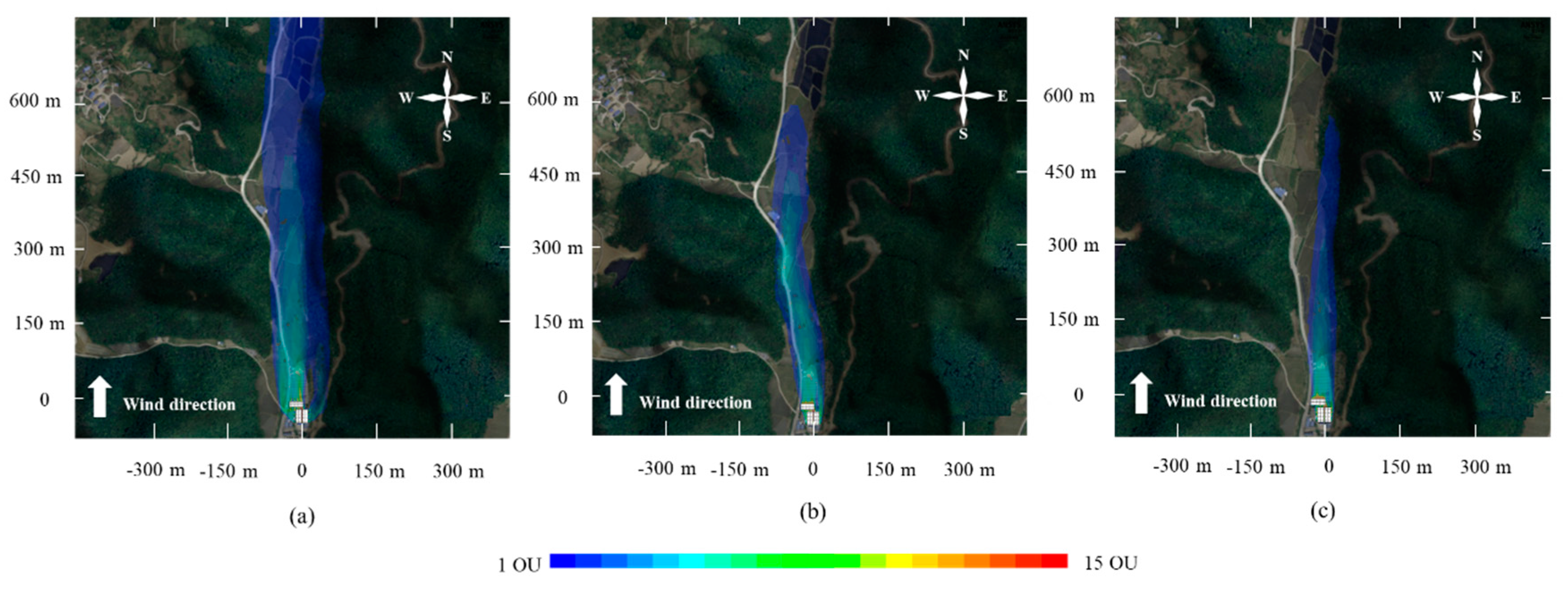
3.3.3. Effect of Wind Speed in Odour Dispersion

Under the same simulation conditions, the average odour dispersion distance was 511.3 m at 0.5 m s⁻¹ of wind speed, and it was calculated as 247.4 m at 1.5 m s⁻¹ and 195.6 m at 2.5 m s⁻¹. At 2.5 m s⁻¹ wind speed, the dispersion distance was reduced by an average of 61.7% compared with 0.5 m s⁻¹. As the wind speed increased, the dispersion distance of odour emitted from pig houses decreased. This trend was mentioned in the studies of Chastain and Wolak [22], Guo et al. [62], Xing [63], and Heinemann and Wahanik [64]. Figure 11 represented CFD-computed results of odour dispersion for various wind speeds under the conditions that pig houses used the sidewall exhaust fan, the wind direction was southerly wind, and the atmospheric stability was stable. Indeed, the odour dispersed farther at high wind speeds, but the dispersed odour was more diluted with external air, so the odour dispersion distance seemed to decrease as the odour concentration dropped below the human perception limit. In addition, when the odour was continuously emitted from the pig houses and the wind was constantly blown at a specific wind speed and in a specific wind direction, the smaller the wind speed, the larger the horizontal dispersion width (left and right) from the outlet, as shown in Figure 11. On the contrary, when the wind speed around the pig houses increased, the odour dispersion to the horizontal direction did not occur much. The dispersion width at the lowest wind speed was 132.71 m; this is higher by 8.1% and 179.5% compared with the dispersion width when wind speed was 1.5 m s⁻¹ (122.8 m) and 2.5 m s⁻¹ (47.5 m), respectively.

3.3.4. Effect of Wind Direction in Odour Dispersion

Wind direction is also an important weather factor that determines the direction of odour dispersion. This wind direction is greatly influenced by the surrounding topography. Therefore, when considering the wind direction, it must be explained along with the complex terrain. The average dispersion distances for wind directions (north, east, south, and west) were calculated to be 369.0, 197.8, 470.5, and 235.1 m, respectively. The CFD-computed results showed that the odour dispersion distances were longer with a southerly wind and with the northerly wind at any atmospheric stability, ventilation type, and wind speed because there are no obstacles with high altitude, such as mountains and hills on the windward and leeward. When the northerly wind was generated, the average odour distance was 21.6% lower than that of the southerly wind. The reason for this was that there were no obstacles to the north from the pig house, but the mountain area was located at about 400 m away from the pig house in the south, which may affect the dispersion of odour. In the same way, the wind speed near the ground of southerly wind was lower than the speed of northerly wind because the wind did not recover from the height near the farm due to the mountain located at the southern part of the domain. Additionally, when the westerly wind was formed, the odour dispersion distance was increased by 18.8% compared with the easterly wind. This result was influenced by the steep slope of the mountain along the western direction (approximately 49.2%) compared with the slope of the mountain along the eastern direction (38.5%), which limits the transports of odours farther from the pig farm. Figure 12 showed the vector field around experimental pig houses under easterly wind conditions. As shown in the figure, when the wind originated from the eastern part of the computational domain, the wind passed through a mountain first before reaching the pig houses.

3.4. Statistical Analysis for Odour Dispersion

Multiple regression analyses were performed to estimate the odour dispersion distance depending on ventilation type, atmospheric stability, wind speed, and wind direction. In this study, the atmospheric stability, ventilation type, and wind direction were nominal variables, while both wind speed and the odour dispersion distance were scale variables. Therefore, a total of seven dummy variables were adopted in the statistical analysis of the CFD-computed results. In the analysis, dummy variable (a) was used to represent the statistical difference between the effect of sidewall exhaust fan and roof-chimney exhaust fan; dummy variable (b) was used to represent the statistical difference between the effect of sidewall exhaust fan and the combined sidewall–roof-chimney exhaust fan. The dummy variable (c) was used to evaluate the statistical difference in the effect between stable atmospheric stability and neutral atmospheric stability; dummy variable (d) was used to evaluate the statistical difference in the effect between stable atmospheric stability and unstable atmospheric stability. To represent the statistical difference to north wind direction with other wind directions, dummy variables (e), (f), and (g) representing east, south, and west directions were used. The independent variable used includes speed, dummy variable (a), (b), (c), (d), (e), (f), and (g), while the dependent variable was the odour dispersion distance.

In the multicollinearity test, which was first conducted prior to the statistical analysis, the calculated VIF values were below 10 for each independent variable, indicating no significant relationship between variables. To determine the appropriate model to predict odour dispersion distance, a backward elimination process was implemented. As shown in

Table 7. Computed R, R², and adjusted R² values from the multiple regression analysis of odour dispersion distance.

Model	Independent Variable	R	R2	Adjusted R2
1	speed, dummy variable d	0.508	0.259	0.252
2	speed, dummy variable d, f	0.622	0.386	0.375
3	speed, dummy variable d, f, a	0.712	0.507	0.493
4	speed, dummy variable d, f, a, b	0.736	0.542	0.524
5	speed, dummy variable d, f, a, b, e	0.789	0.622	0.603
6	speed, dummy variable d, f, a, b, e,	0.806	0.650	0.629
7	speed, dummy variable d, f, a, b, e, g	0.828	0.685	0.663

, the R² and the adjusted R² value for the model with a lesser number of independent variables were lower compared with the models considering a greater number of independent variables. The linear regression equation derived is shown in Table 7 with an R² value and adjusted R² value of 0.685 and 0.663, respectively, for odour dispersion distance. In the regression analysis, the change between stable and neutral atmospheric stability (dummy variable c) showed a very small t-value of −0.409. In addition, the calculated p-value for the dummy variable (c) was found to be insignificant at p < 0.05, with a value of 0.683. This means that the change in dummy variable (c) is not associated with the changes in the dependent variable because no significant difference was found between the cases having an atmospheric stability of stable and neutral. Thus, the dummy variable representing the effect of stable and neutral conditions (dummy variable c) was excluded from the independent variables and regression analysis was recalculated.

The results of the regression analysis in

Table 8. Computed regression coefficients, standard errors, t-values, and p-values from the multiple regression analysis of odour dispersion distance with selected variables.

Odour Dispersion Distance	Unstandardized Coefficients		Standardized Coefficients	t-Value	p-Value
	Coefficient	Std. Error	Coefficient
(Intercept)	791.108	44.718		17.691	1.46 × 10−32
Speed	−157.849	17.428	−0.508	−9.057	1.15 × 10−14
dummy variable a	−188.733	34.857	−0.351	−5.415	4.23 × 10−7
dummy variable b	−175.188	34.857	−0.326	−5.026	2.20 × 10−6
dummy variable d	−192.199	30.187	−0.357	−6.367	5.90 × 10−9
dummy variable e	−171.123	40.249	−0.292	−4.252	4.78 × 10−5
dummy variable f	101.513	40.249	0.173	2.522	0.0013
dummy variable g	−133.853	40.249	−0.229	−3.326	0.001

showed that all the independent variables are significant at a confidence level of 95%. Furthermore, the wind speed has the highest t-value and lowest p-value of −9.057 and 1.15 × 10⁻¹⁴, respectively. This indicated that an abrupt change in wind speed can substantially affect the dispersion of odour along downwind. The influence of atmospheric stability was also found to have t and p-values of −6.367 and 5.90 × 10⁻⁹. The vertical movement of odorous parcels caused by the stability and instability of the atmospheric stability has a large impact on the dispersion of odour. Meanwhile, dummy variables (a) and (b) representing the statistical difference between the effect of using a sidewall exhaust fan and other ventilation systems showed almost identical t-values of −5.415 (dummy variable a) and −5.026 (dummy variable c). The odour dispersion distance can be predicted using the model shown below (Equation (16)).

$$\begin{array}{cc}\hfill \mathrm{Odour} \mathrm{dispersion}& \mathrm{distance}\hfill \\ & =791.108-(157.849\times \mathrm{speed})-(192.199\times \mathrm{dummy} \mathrm{variable} \mathrm{d})\hfill \\ & -(188.733\times \mathrm{dummy} \mathrm{variable} \mathrm{a})+(175.188\times \mathrm{dummy} \mathrm{variable} \mathrm{b})\hfill \\ & -(171.123\times \mathrm{dummy} \mathrm{variable} \mathrm{e})-(133.853\times \mathrm{dummy} \mathrm{variable} \mathrm{g})\hfill \\ & +(101.513\times \mathrm{dummy} \mathrm{variable} \mathrm{f})\hfill \end{array}$$

(16)

To supplement the regression analysis in identifying the key factors affecting the dispersion of odour outside the pig farm, a relative weight analysis on the independent variable was used. The calculated R² was 0.44 and the confidence level was set at 95%. The result of the analysis summarized in

Table 9. Relative weight analysis of independent variables in odour dispersion distance.

Variable	Raw Relative Weight	Rescaled Relative Weight (%)
ventilation type	0.080	17.91
atmospheric stability	0.103	23.20
wind speed	0.259	58.17
direction	0.003	0.73

showed a similar trend in terms of independent variables’ ranking with regard to contribution to odour prediction. In the RWA method, the wind speed was the most influential factor that contributes to odour dispersion, followed by the atmospheric stability, ventilation type, and wind direction, with rescaled relative weight values of 58.2%, 23.2%, 17.9%, and 0.7%, respectively.

4. Discussion

Unlike typical results showing higher accuracy in a simulation using the LES turbulence model, the LES model showed a higher error compared with other turbulence models. This may be due to the y+ value related to mesh resolution. In the case of the LES turbulence model, the y+ value should be designed to be 1 or less. However, it was difficult to satisfy this criterion when considering the size of the target computational domain in this study. Therefore, unlike the RANS models (standard k-ε model, RNG k-ε model, and standard k-ω model), the LES model did not fully meet the criteria for the y+ value. Although the y+ design criterion was not met, the CFD-computed result using LES models was expected to have an accurate result. Thus, in this study, the LES model was used as a turbulence model for validating the three-dimensional model. However, contrary to the expected results, the LES model showed a rather low accuracy. If the y+ criterion is not met, it is thought that it can show lower accuracy than the RANS model in terms of accuracy. Among the RANS model, the standard k-ε turbulence model has been widely used in various CFD studies due to its relative simplicity, robustness, ease of usage, lesser computational requirements, and its applicability to various flows. Therefore, the standard k-ε turbulence model was applied in this study.

The difference in the odour dispersion distance according to the ways (ventilation method; sidewall exhaust fan; roof-chimney exhaust fan) of applying the exhaust fan of the pig house varied from 16.8% to 61.7%. The reason was that there was a difference in the odour concentration at the height of the receptor according to the effect of the shield installed on the roof-chimney exhaust fan and the height difference of the outlet. when the sidewall exhaust fan was used, the odorous air emitted directly travelled away from that source at a constant rate with no vortex formation (Figure 13a). In the case of a roof-chimney exhaust fan, a vortex was formed around the shield of the exhaust fan reducing the concentration of the odour emitted (Figure 13b). The vortex created initiated the mixing of the air with the odorous air emitted from the pig house causing lower dispersion distance of odour.

There was no significant difference between stable and neutral conditions in the stability of the atmosphere. The same trend result was found in the odour dispersion modelling result [20,45,60]. The not significant difference between the result of neutral and stable atmospheric stability is due to equal or lower temperature of odorous parcel compared with the surrounding temperature allowing the pollutants to remain on the ground. For the dispersion width, the difference can be explained by the turbulent mixing that happened at unstable atmospheric stability commencing the movement of odorous compounds to move in all directions. Thus, the odorous air was easily diluted with air and became less detectable in the leeward direction. In addition, the odour dispersed farther at high wind speeds, but the dispersed odour was more diluted with external air, so the odour dispersion distance seemed to decrease as the odour concentration dropped below the human perception limit.

Surrounding complex terrain and mountain affected the dispersion distance; since the pig house was less than 100 m away from the foot of the hill along with the eastern domain, the wind was not strong enough to lift and transport the odorous substances away from the source. Specifically, when the wind from this direction flowed through the mountains, the wind accelerated uphill and decelerated near the downhill slopes. After the wind passed through the mountains, its momentum was reduced, resulting in lower wind speed. This causes lower dispersion at easterly and westerly wind directions.

5. Conclusions

The rapid intensification in pig production has led to an increase in livestock pollutant emissions. For this reason, attempts are being made to study the influence of various environmental conditions on odour dispersion. With the advancement of technology and computer software, dispersion models were one of the most common methods to visualize and estimate odour occurrences. Therefore, a three-dimensional model containing a complex terrain was developed in this study to realise odour dispersion originating from pig houses.

The CFD-computed results showed that odour dispersion distance at the level of 1 OU m⁻³ ranged from 78.9 to 1488.1 m. When using an exhaust fan on the sidewall, the odour dispersion ranged from 147.8 to 1488.1 m, depending on the simulated environmental conditions. On the other hand, the roof-chimney exhaust fan showed a minimum of 78.1 to 900.6 m. There was an average difference of 41.3% (maximum: 61.7%, minimum: 16.8%) dispersion distance, depending on the physical environment (ventilation method; sidewall exhaust fan; roof-chimney exhaust fan). Moreover, when the sidewall exhaust fan and the chimney exhaust fan were used simultaneously, the odour dispersion distance was estimated to be 5.4% larger than that of the exhaust using only the roof-chimney exhaust fan. It was shown that the application of a sidewall exhaust fan can significantly affect the height of the receptor. However, when internal air exhausted through a roof-chimney exhaust fan, the effect was relatively lower at the height of the receptor due to the turbulent mixing in the atmosphere and the duct shield. The average odour dispersion distance was 511.3 m at 0.5 m s⁻¹ of wind speed, and it was calculated as 247.4 m at 1.5 m s⁻¹ and 195.6 m at 2.5 m s⁻¹. As the wind speed increased, the dispersing distance of odour emitted from the pig houses decreased; the smaller the wind speed, the larger the horizontal dispersion width (left and right) from the outlet. On the contrary, when the wind speed around the pig houses increased, the odour dispersion to the horizontal direction did not occur much. The average dispersion distances for wind directions (north, east, south, and west) were calculated to be 369.0, 197.8, 470.5, and 235.1 m, respectively. Depending on the complex terrain and obstacle conditions, the dispersing distance of the odour emitted from the pig house varies. Particularly, the difference in the dispersion distance of odour could occur depending on the slope of the mountain that surrounds the pig house. In addition, the statistical analysis result showed that the wind speed was the most influential factor that affects odour dispersion outside the pig house facility followed by atmospheric stability, ventilation type, and wind direction. It is considered that the influence of these environmental variables can be used as fundamental information for farm location selection, ventilation control design, and operation method.

References

1. Statistics Korea. 2020. Available online: http://kostat.go.kr (accessed on 3 January 2020).
2. Statistics Korea. 2019. Available online: http://kostat.go.kr (accessed on 21 November 2019).
3. Ministry of Environment. Available online: https://eng.me.go.kr (accessed on 12 November 2019).
4. Bottcher, R.; Munilla, R.; Baughman, G.; Keener, K. Designs for windbreak walls for mitigating dust and odor emissions from tunnel ventilated swine buildings. In Proceedings of the Swine Housing Conference, Des Moines, IA, USA, 9–11 October 2000; p. 1. [Google Scholar]
5. Colletti, J.; Hoff, S.; Thompson, J.; Tyndall, J. Vegetative environmental buffers to mitigate odor and aerosol pollutants emitted from poultry production sites. In Proceedings of the Workshop on Agricultural Air Quality: State of Science, Potomac, MD, USA, 4–8 June 2006; pp. 5–8. [Google Scholar]
6. Rzeźnik, W.; Mielcarek-Bocheńska, P. Effect of the slurry application method on odour Emissions: A pilot study. Pol. J. Environ. Stud. 2020, 29, 1503–1509. [Google Scholar] [CrossRef]
7. Choi, E.; Kim, J.; Choi, I.; Ahn, H.; Dong, J.I.; Kim, H. Microbial additives in controlling odors from stored swine slurry. Water Air Soil Pollut. 2015, 226, 104. [Google Scholar] [CrossRef]
8. Ha, D.-M.; Kim, D.-H. Effects of the Liquid Manure Circulation System on the Environmental Improvement of Swine Farm. J. Environ. Sci. Int. 2019, 28, 137–145. [Google Scholar]
9. Hartung, E.; Jungbluth, T.; Bascher, W. Reduction of ammonia and odor emissions from a piggery with biofilters. Trans. ASAE 2001, 44, 113. [Google Scholar] [CrossRef]
10. Lim, T.-T.; Jin, Y.; Ni, J.-Q.; Heber, A.J. Field evaluation of biofilters in reducing aerial pollutant emissions from a commercial pig finishing building. Biosyst. Eng. 2012, 112, 192–201. [Google Scholar] [CrossRef]
11. McCrory, D.F.; Hobbs, P. Additives to Reduce Ammonia and Odor Emissions from Livestock Wastes: A Review. J. Environ. Qual. 2001, 30, 345–355. [Google Scholar] [CrossRef] [Green Version]
12. Melse, R.W.; Hol, J.M. Biofiltration of exhaust air from animal houses: Evaluation of removal efficiencies and practical experiences with biobeds at three field sites. Biosyst. Eng. 2017, 159, 59–69. [Google Scholar] [CrossRef]
13. Hong, S.; Lee, E. Study on the reduction of livestock malodor using microbial agents-focusing on swine facilities. J. Odor Indoor Environ. 2018, 17, 85–94. [Google Scholar] [CrossRef]
14. Yoo, J.; Suh, J.; Lee, E. Study on the Reduction of Malodor Produced from Pig Excreata using Microbial Agents. Korean J. Odor Res. Eng. 2010, 9, 203–207. [Google Scholar]
15. Zhao, Y.; Aarnink, A.; De Jong, M.; Ogink, N.; Koerkamp, P. Effectiveness of multi-stage scrubbers in reducing emissions of air pollutants from pig houses. Trans. ASABE 2011, 54, 285–293. [Google Scholar] [CrossRef]
16. National Institute of Environment Research (NEIR). Available online: https://www.nier.go.kr (accessed on 21 December 2019).
17. Ambient Air-Determination of Odour in Ambient Air by Using Field Inspection-Part 1: Grid Method, EN 16841-1; European Committee for Standardization CEN: Brussels, Belgium, 2016.
18. Yeo, U.-H.; Lee, I.-B.; Ha, T.-H.; Decano, C.; Kim, R.-W.; Lee, S.-Y.; Kim, J.-G.; Choi, Y.-B.; Park, Y.-M. Evaluation of Odor Dispersion from Livestock Building through Field Experiment. Korean Soc. Agric. Eng. 2019, 61, 21–30. [Google Scholar]
19. Sironi, S.; Capelli, L.; Céntola, P.; Del Rosso, R.; Pierucci, S. Odour impact assessment by means of dynamic olfactometry, dispersion modelling and social participation. Atmos. Environ. 2010, 44, 354–360. [Google Scholar] [CrossRef]
20. Hong, S.; Lee, I.; Hwang, H.; Seo, I.; Bitog, J.; Kwon, K.; Song, J.; Moon, O.; Kim, K.; Ko, H. CFD modelling of livestock odour dispersion over complex terrain, part II: Dispersion modelling. Biosyst. Eng. 2011, 108, 265–279. [Google Scholar] [CrossRef]
21. Guo, H.; Yu, Z.; Lague, C. Livestock odour dispersion modeling: A review. In Proceedings of the 2006 ASAE Annual Meeting, Edmonton, AB, Canada, 16–19 July 2006; p. 1. [Google Scholar]
22. Chastain, J.P.; Wolak, F.J. Application of a Gaussian plume model of odor dispersion to select a site for livestock facilities. In Proceedings of the Odors and VOC Emissions 2000 Conference, Cincinnati, OH, USA, 16–19 April 2000; pp. 745–758. [Google Scholar]
23. Carlson, J.; Arndt, D.S. The Oklahoma Dispersion Model: Using the Gaussian plume model as an operational management tool for determining near-surface dispersion conditions across Oklahoma. J. Appl. Meteorol. Climatol. 2008, 47, 462–474. [Google Scholar] [CrossRef]
24. Schulte, D.D.; Modi, M.R.; Henry, C.G.; Billesbach, D.P.; Stowell, R.R.; Hoff, S.J.; Jacobson, L.D. Modeling odor dispersion from a swine facility using AERMOD. In Proceedings of the International Symposium on Air Quality and Waste Management for Agriculture, Broomfield, CO, USA, 16–19 September 2007; p. 64. [Google Scholar]
25. Busini, V.; Capelli, L.; Sironi, S.; Nano, G.; Rossi, A.N.; Bonati, S. Comparison of CALPUFF and AERMOD models for odour dispersion simulation. Chem. Eng. Trans. 2012, 30, 1–6. [Google Scholar]
26. Sheridan, B.; Hayes, E.; Curran, T.; Dodd, V. A dispersion modelling approach to determining the odour impact of intensive pig production units in Ireland. Bioresour. Technol. 2004, 91, 145–152. [Google Scholar] [CrossRef]
27. Zhu, J.; Jacobson, L.D.; Schmidt, D.R.; Nicolai, R. Evaluation of INPUFF-2 model for predicting downwind odors from animal production facilities. Appl. Eng. Agric. 2000, 16, 159–164. [Google Scholar] [CrossRef]
28. Capelli, L.; Sironi, S.; Del Rosso, R.; Guillot, J.-M. Measuring odours in the environment vs. dispersion modelling: A review. Atmos. Environ. 2013, 79, 731–743. [Google Scholar] [CrossRef]
29. Lin, X.-J.; Barrington, S.; Nicell, J.; Choiniere, D.; Vezina, A. Influence of windbreaks on livestock odour dispersion plume in the field. Agric. Ecosyst. Environ. 2006, 116, 263–272. [Google Scholar] [CrossRef]
30. Chastain, J.P. Air quality and odor control from swine production facilities. In Confined Animal Manure Managers Certification Program Manual; Clemson University: Clemson, SC, USA, 1999; pp. 9.1–9.11. [Google Scholar]
31. Stockie, J.M.J.S.R. The mathematics of atmospheric dispersion modeling. SIAM Rev. 2011, 53, 349–372. [Google Scholar] [CrossRef]
32. Sánchez-Sosa, J.E.; Castillo-Mixcóatl, J.; Beltrán-Pérez, G.; Muñoz-Aguirre, S. An Application of the Gaussian Plume Model to Localization of an Indoor Gas Source with a Mobile Robot. Sensors 2018, 18, 4375. [Google Scholar]
33. Conti, C.; Guarino, M.; Bacenetti, J. Measurements techniques and models to assess odor annoyance: A review. Environ. Int. 2020, 134, 105261. [Google Scholar] [CrossRef] [PubMed]
34. Cao, S. CFD applications in structural wind engineering. In Advanced Structural Wind Engineering; Springer: Heidelberg, Germany, 2013; pp. 301–324. [Google Scholar]
35. Stergiannis, N.; Lacor, C.; Beeck, J.; Donnelly, R. CFD modelling approaches against single wind turbine wake measurements using RANS. In Proceedings of the Journal of Physics: Conference Series; IOP Publishing: Brussel, Belgium, 2016; Volume 753, p. 032062. [Google Scholar]
36. Vilag, V.; Vilag, J.; Carlanescu, R.; Mangra, A.; Florean, F. CFD Application for Gas Turbine Combustion Simulations. In Computational Fluid Dynamics Simulations; IntechOpen: London, UK, 2019. [Google Scholar]
37. Ardejani, F.D.; Baafi, E.; Panahi, K.S.; Singh, R.N.; Shokri, B.J. Application of Computational Fluid Dynamics (CFD) for simulation of acid mine drainage generation and subsequent pollutants transportation through groundwater flow systems and rivers. In Computational Fluid Dynamics Technologies and Applications; IntechOpen: London, UK, 2011; pp. 123–160. [Google Scholar]
38. Modenesi, K.; Furlan, L.; Tomaz, E.; Guirardello, R.; Núnez, J. A CFD model for pollutant dispersion in rivers. Braz. J. Chem. Eng. 2004, 21, 557–568. [Google Scholar] [CrossRef] [Green Version]
39. Zárate, L.G.; Uribe, S.; Cordero, M.E. Applications of CFD for Process Safety. In Computational Fluid Dynamics-Basic Instruments and Applications in Science; IntechOpen: London, UK, 2017. [Google Scholar]
40. Selmi, M.; Belmabrouk, H.; Bajahzar, A. Numerical Study of the Blood Flow in a Deformable Human Aorta. Appl. Sci. 2019, 9, 1216. [Google Scholar] [CrossRef] [Green Version]
41. Shin, E.; Kim, J.J.; Lee, S.; Ko, K.S.; Rhee, B.D.; Han, J.; Kim, N. Hemodynamics in diabetic human aorta using computational fluid dynamics. PLoS ONE 2018, 13, e0202671. [Google Scholar] [CrossRef]
42. Suzelle, B.; Jun, L.X.; Denis, C. Simulating Odour Dispersion about Natural Windbreaks. Comput. Fluid Dyn. Technol. Appl. 2011, 181, 182–215. [Google Scholar]
43. Bjerg, B.; Kai, P.; Morsing, S.; Takai, H. CFD analysis to predict close range spreading of ventilation air from livestock buildings. Agric. Eng. Int.: CIGR J. 2004, 6, 1–12. [Google Scholar]
44. Bonifacio, H.F.; Maghirang, R.G.; Glasgow, L.A. Numerical simulation of transport of particles emitted from ground-level area source using AERMOD and CFD. Eng. Appl. Comput. Fluid Mech. 2014, 8, 488–502. [Google Scholar] [CrossRef] [Green Version]
45. Li, Y.; Guo, H. Comparison of odor dispersion predictions between CFD and CALPUFF models. Trans. ASABE 2006, 49, 1915–1926. [Google Scholar] [CrossRef]
46. Lin, X.-J.; Barrington, S.; Choiniere, D.; Prasher, S. Effect of weather conditions on windbreak odour dispersion. J. Wind. Eng. Ind. Aerodyn. 2009, 97, 487–496. [Google Scholar] [CrossRef]
47. Riddle, A.; Carruthers, D.; Sharpe, A.; McHugh, C.; Stocker, J. Comparisons between FLUENT and ADMS for atmospheric dispersion modelling. Atmos. Environ. 2004, 38, 1029–1038. [Google Scholar] [CrossRef]
48. Diego, I.; Pelegry, A.; Torno, S.; Toraño, J.; Menendez, M. Simultaneous CFD evaluation of wind flow and dust emission in open storage piles. Appl. Math. Model. 2009, 33, 3197–3207. [Google Scholar] [CrossRef]
49. Katsanis, S. Numerical Modelling of Wind Borne Pollution Dispersion from Open Windrow Compost Sites. Ph.D. Thesis, University of Sheffield, Sheffield, UK, 23 March 2014. [Google Scholar]
50. Úbeda Sánchez, Y.; López Jiménez, P.A.; Nicolas, J.; Calvet Sanz, S. Strategies to control odours in livestock facilities: A critical review. Span. J. Agric. Res. 2013, 11, 1004–1015. [Google Scholar] [CrossRef]
51. Hong, S.-W.; Lee, I.-B.; Seo, I.-H.; Bitog, J.; Kwon, K.-S. Prediction of livestock odour dispersion over complex terrain using CFD technology: Review and simulation study. In Proceedings of the Ist International Symposium on CFD Applications in Agriculture, Valencia, Spain, 9–10 July 2012; pp. 29–36. [Google Scholar]
52. Appropriate Livestock Raising Standard per Unit Area of Livestock Raising Facility. Available online: http://www.law.go.kr (accessed on 2 March 2020).
53. Jang, J.; Jin, X.; Hong, J.; Kim, Y. Effects of different space allowances on growth performance, blood profile and pork quality in a grow-to-finish production system. Asian-Australas. J. Anim. Sci. 2017, 30, 1796–1802. [Google Scholar] [CrossRef] [PubMed] [Green Version]
54. Ministry of Agriculture, Food and Rural Affairs (MAFRA). Available online: http://www.mafra.go.kr (accessed on 2 March 2020).
55. ANSYS Fluent Tutorial Guide 18; ANSYS Inc.: Canonsburg, PA, USA, 2018; pp. 724–746.
56. Dyer, A.; Hicks, B. Flux-gradient relationships in the constant flux layer. Q. J. R. Meteorol. Soc. 1970, 96, 715–721. [Google Scholar] [CrossRef]
57. Hicks, B. Wind profile relationships from the ‘Wangara’ experiment. Q. J. R. Meteorol. Soc. 1976, 102, 535–551. [Google Scholar]
58. Bache, D.H.; Johnstone, D.R. Microclimate and Spray Dispersion; Ellis Horwood: West Sussex, UK, 1992. [Google Scholar]
59. ASHRAE. Standard 62-1989, Ventilation for Acceptable Indoor Air Quality; American Society of Heating, Refrigeration, and Air Conditioning Engineers: Atlanta, GA, USA, 1989. [Google Scholar]
60. Power, V.; Stafford, T. Odour Impacts and Odour Emission Control Measures for Intensive Agriculture; EPA: Wexford, Ireland, 2001.
61. Tonidandel, S.; LeBreton, J.M. Relative importance analysis: A useful supplement to regression analysis. J. Bus. Psychol. 2011, 26, 1–9. [Google Scholar] [CrossRef]
62. Guo, H.; Jacobson, L.D.; Schmidt, D.R.; Janni, K. Simulation of Odor Dispersions as Impacted by Weather Conditions. In Proceedings of the Livestock Environment VI: Proceedings of the 6th International Symposium 2001, Louisville, KY, USA, 21–23 May 2001; pp. 687–695. [Google Scholar]
63. Xing, Y.; Guo, H.; Feddes, J.; Yu, Z.; Shewchuck, S.; Predicala, B. Sensitivities of four air dispersion models to climatic parameters for swine odor dispersion. Trans. ASABE 2007, 50, 1007–1017. [Google Scholar] [CrossRef]
64. Heinemann, P.; Wahanik, D. Modeling the generation and dispersion of odors from mushroom composting facilities. Trans. ASAE 1998, 41, 437–446. [Google Scholar] [CrossRef]
Figure 1. Research flow for identifying key factors influencing odour dispersion emitted from a pig farm. CFD—computational fluid dynamics.
Agronomy 10 01828 g001
Figure 2. Experimental pig houses. (a) Satellite image around the pig farm (b) outside the pig house, and (c) inside the pig house [18].
Agronomy 10 01828 g002
Figure 3. Schematic diagram of a standard pig house used in the CFD simulation and designed CFD model. (a) Side view of standard pig house, (b) front view of standard pig house, and (c) designed CFD model in the computational domain.
Agronomy 10 01828 g003
Figure 4. Field experiment inside and outside the pig house. (a) Installation of ammonia and odour sampling device inside the pig house, (b) installation of ammonia and odour sampling device outside the pig house, (c) external weather measurement device installed on the roof of the pig house, and (d) measurement of atmospheric stability using a balloon with temperature sensors.
Agronomy 10 01828 g004
Figure 5. Locations of sampling and measurement instruments inside and outside the pig houses.
Agronomy 10 01828 g005
Figure 6. Design of CFD model for estimation of odour dispersion from the experimental pig house.
Agronomy 10 01828 g006
Figure 7. Space segmentation to reduce the number of grids designed in the computational domain and improve the grid quality.
Agronomy 10 01828 g007
Figure 8. The installation location of a hot wire anemometer for measuring exhaust air flow.
Agronomy 10 01828 g008
Figure 9. Odour dispersion according to ventilation type at stable condition with 1.5 m s−1 wind speed and northerly wind. (a) Sidewall exhaust fan. (b) Roof-chimney exhaust fan.
Agronomy 10 01828 g009
Figure 10. Odour dispersion using sidewall exhaust with a southerly wind and wind speed of 1.5 m s−1. (a) Stable condition and (b) unstable condition.
Agronomy 10 01828 g010
Figure 11. Odour dispersion using sidewall exhaust ventilation based on wind direction with southerly wind. (a) 0.5 m s−1, (b) 1.5 m s−1, and (c) 2.5 m s−1.
Agronomy 10 01828 g011
Figure 12. Vector field in the mountains of the east and west of the pig houses (easterly wind).
Agronomy 10 01828 g012
Figure 13. Vector flow according to ventilation type at the stable condition with 1.5 m s−1 wind speed, and northerly wind. (a) Sidewall exhaust fan, (b) roof-chimney exhaust.
Agronomy 10 01828 g013