Article

Assessing the Sensitivity of Site-Specific Lime and Gypsum Recommendations to Soil Sampling Techniques and Spatial Density of Data Collection in Australian Agriculture: A Pedometric Approach

by
Stirling D. Roberton
1,*,
John McL. Bennett
1,
Craig R. Lobsey
1 and
Thomas F. A. Bishop
2
1
Centre for Sustainable Agricultural Systems, University of Southern Queensland, West St, Toowoomba 4350, Queensland, Australia
2
Department of Environmental Science, Faculty of Agriculture and Environment, The University of Sydney, Biomedical Building C81, 1 Central Avenue, Eveleigh, Sydney 2015, NSW, Australia
*
Author to whom correspondence should be addressed.
Agronomy 2020, 10(11), 1676; https://doi.org/10.3390/agronomy10111676
Submission received: 22 September 2020 / Revised: 21 October 2020 / Accepted: 22 October 2020 / Published: 29 October 2020
(This article belongs to the Special Issue Smart Decision-Making Systems for Precision Agriculture)

Abstract

:
There is currently limited understanding surrounding the spatial accuracy of soil amelioration advice as a function of sampling density at the sub-field scale. Consequently, soil-based decisions are often made using a data limiting approach, as the value proposition of soil data collection has not been well described. The work presented here investigates the spatial errors of gypsum and lime recommendations based on industry-standard blanket-rate and zone-based variable rate application, as well as the more advanced pedometric approaches—ordinary kriging (OK) and regression kriging (RK). All methods were tested at sampling densities between 0.1–3 samples/ha for a 108 ha broadacre site in central NSW, Australia. Whilst previous work has tested the effect of sampling density on the spatial predictive performance of OK and RK, here we assess prediction accuracy as the error associated with soil management decisions based on their results (i.e., the over- and under-application error of gypsum and lime applications) in conjunction with the RMSE of prediction for soil pH and exchangeable sodium percentage (ESP). The uncertainty of each method is also tested to observe the effect of random initialisation on predictive performance. Results indicated that RK provided superior spatial predictions across all sampling densities for the application of gypsum and lime, with a blanket-rate application providing the worse results, with over- and under-application errors exceeding 200 t and 300 t respectively for 40–60 cm treatment for the entire field. Interestingly, the spatial accuracy of amendment application increased to a sampling density of 0.5 samples/ha for RK, with minimal improvement thereafter, suggesting that meaningful soil amelioration advice can be attained proximal to this density.

1. Introduction

Site-specific agronomic decisions are often made using limited soil information, due to the perceived cost of soil data acquisition in relation to its perceived usefulness [1,2,3]. When diagnosing soil constraints, agricultural practitioners will typically use surface-based “grab samples” i.e., 0–10 cm depth along a transect, which is then bulked prior to analysis to derive a single representation of field condition. This subsequently results in ‘blanket-rate’ (BR) amelioration, whereby a single amendment rate is applied across the field, irrespective of spatial soil variation. Whilst this approach represents the current practice in the industry, there is limited understanding surrounding the economic and agronomic consequences of decisions made in such a data-limited environment. More specifically, there has been limited assessment of the error in agronomic recommendations at different sampling densities. These errors may be highly influential on overall farm profitability, as large soil treatment investments are often made on these recommendations [4,5]. Furthermore, there is an emerging social responsibility for advisors and land-owners to ensure appropriate management of farming inputs to match soil conditions [6,7,8]. It is therefore important to understand how both the spatial variability of soil constraints and soil sampling regimes will influence amendment application outcomes that are simultaneously profitable and socially responsible.
A more pragmatic approach to sub-field constraint management is sampling designs that facilitate ‘variable-rate’ amelioration, whereby the rate of ameliorant is spatially matched to the soil condition. In the presence of auxiliary information such as environmental covariates (e.g., crop yield data, remotely sensed data, proximally sensed data etc.), this may be achieved by taking a clustering approach, whereby a field is stratified into discrete spatial strata, commonly referred to as management zones [9]. Samples are then randomly selected within each strata and bulked to provide a strata-average of soil condition. Whilst the approach was largely used to identify and map soil classes across a landscape, [10,11,12,13], merit exists in applying the approach to identify soil classes at fine scale (i.e., within a single field). Clustering for zone-based management is the currently accepted standard for variable-rate management in commercial precision agriculture [14,15], although the inability to map continuous soil properties significantly reduces the capacity for true precision management.
Geostatistical or model-based digital soil mapping (DSM) techniques offer advancement to true variable-rate soil management which facilitates the mapping of soil variables at a continuous scale. Geostatistical approaches such as ordinary kriging (OK) [16] are widely used to interpolate spatial data for soil management. Optimal sampling designs for OK predictions aim to maximise coverage within the geographic space, using a regular grid [17,18,19], or stratified random sampling design [20].
In the presence of environmental covariates, model-based approaches such as regression kriging (RK) generally provide improved spatial predictions over OK [21,22,23,24]. These improvements are derived where soil variation is correlated with the available environmental covariates [25]. RK performs spatial predictions by firstly modelling the measured soil properties as a function of the environmental covariates at the sampled locations. This model is then used to predict across unsampled locations. The model’s residual errors are subsequently kriged and added to the predictions to provide a final estimate of the mapped soil property. Soil sampling strategies for RK requires consideration of both the feature space of the environmental covariates and the geographic space. On this basis, conditioned Latin hypercube sampling (cLHS) [26] has become a widely used technique for calibration sample selection in DSM, which selects calibration samples across the feature space of the environmental covariates by considering their multivariate distributions. Whilst RK may provide more accurate spatial predictions, the cost of acquiring environmental covariates and the benefits of improved agronomic decisions must be considered.
While clustering approaches are generally adopted by agricultural practitioners to inform zone-based variable-rate soil constraint management, we contend that there is agronomic merit in increasing the soil sampling and analysis investment to allow for fine-scale soil management. The effect of sampling density and spatial prediction method on agronomic recommendations for constraint amelioration is not well understood. Furthermore, little consideration has been made toward the opportunity cost of incorrect amendment application decisions based on data-limited approaches. Therefore, the aim of this work is to compare the field-scale performance of transect sampling (for BR application), zone-based sampling, OK and RK, at increasing sampling density, for accuracy in soil amelioration recommendations, with a focus on gypsum and lime applications to address sodicity and acidity. Furthermore, we will assess the level of uncertainty surrounding these methods via random initialisation of the search parameters within each method.

2. Materials and Methods

2.1. Experimental Design

A dataset was collected using a 60 m sampling grid to a depth of 60 cm for a 108 ha experimental site, resulting in 300 soil cores with 4 analysis depths (1200 samples in total). This data density was selected as a pragmatic and resource-constrained intensity and used as the baseline of observed variability at the site. Whilst this assumption is clearly incorrect, it was considered reasonable on the basis of being proximal to, if not surpassing, the upper limit of economically feasible sampling density—approximate cost for soil analysis of $833/ha (based on a commercial analysis cost of $75/sample—see www.nutrientadvantage.com.au). The collected dataset was further interpolated to a 6 m grid using RK to form the baseline datasetwhich the identified sampling methods were tested against at increasing sample density. A leave-one-out cross-validation was used to compare the accuracy of OK and RK to interpolate the 6 × 6 m baseline dataset, with RK selected on this basis.
The methods investigated were: (1) random transect sampling, (2) zonal sampling, (3) OK, and (4) RK. Each method was assessed at separate sampling densities of 10, 20, 50, 100, 150, 200, 250, and 300 for the 108 ha site. Each method was applied to create a predicted digital soil map of pH, ESP, CEC and BD at 6 × 6 m pixels, which were used to subsequently make spatial gypsum and lime recommendations. The predicted gypsum and lime recommendations were spatially compared against the baseline DSM. Spatial prediction errors of soil attributes were calculated as:
E r r o r x , y i = a b s P x , y i O x , y i
where P and O are respective predicted and observed values of soil attribute i at grid location x,y. Root-mean square errors (RMSE) were calculated to provide an indication of average error, as well as the standard deviation of the prediction residuals to provide insight into the range of prediction error at each sampling density across the methods. The 4 methods were simulated 50 times at each sampling density to provide insight into the sensitivity of agronomic recommendations to the random initialisation of the methods.

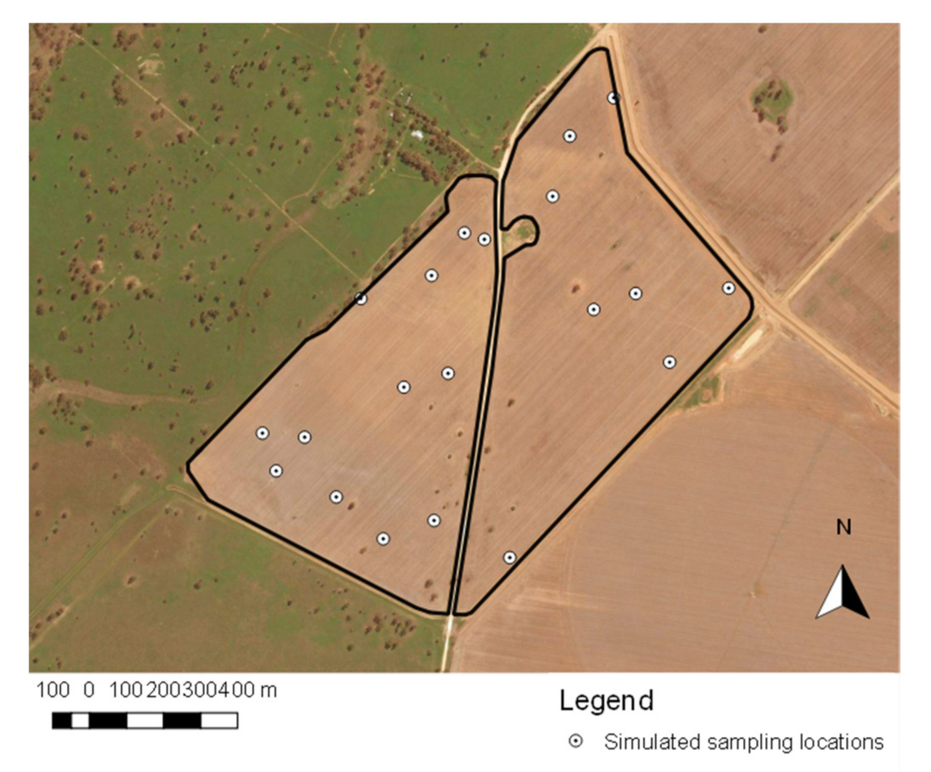
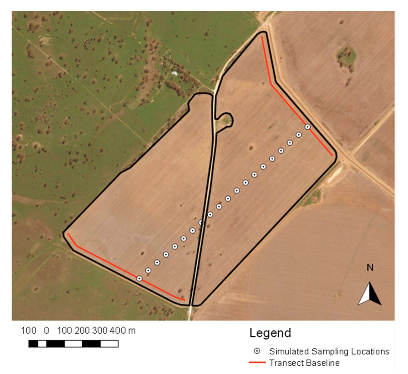
2.2. Investigation Site

The investigation site is located within the Warren district of the Macquarie Valley in central NSW, Australia (GR 31°49′40.49″ S 148°06′44.56″ E). The 108 ha dryland site is managed as a 12 m CTF frontage, zero-tillage farming system and is under a winter cropping rotation consisting of wheat, chickpea and barley. The dominant soil type identified at the site was considered to be Solonetz, with a Cambisol being located toward the south-west [27]. Minimal elevation difference was observed across the site, with the highest and lowest altitude being 211.1 m and 209.4 m AHD respectively. The climate in the Macquarie Valley region is summer rainfall dominant, with average annual rainfall being 413 mm. A mean maximum temperature of 33.6 °C is experienced in January, with the coldest average maximum temperature of 15.5 °C being experienced in July. Near-surface soil geology within the region has been majorly influenced by alluvial processes following the Macquarie River. Soil sampling at the site was undertaken in April of 2017.

2.3. Sampling Methods

The 60 m × 60 m sample grid, provided 300 sample locations for the entire site with two intact soil cores extracted to 60 cm at each site; one for chemical analysis and the other for bulk density (BD) and moisture measurements. Cores were extracted using a core sleeve with an internal cutting tip diameter (ID) of 43 mm on a utility-mounted hydraulic coring apparatus with an attached jackhammer. Each core was sectioned into depths of 0–10 cm, 10–20 cm, 20–40 cm and 40–60 cm, assumed to define the zone of bulk rooting density (i.e., not the extent of rooting) for the crops, and stored in sampling bags. The 1200 samples were measured for soil pH, exchangeable sodium percentage (ESP), BD and cation exchange capacity (CEC), along with other soil structural and chemical measurements not used in this study in accordance with Rayment et al. [28]. A summary of the soil properties used for providing the agronomic recommendations is presented in Table 1.

2.4. Proximally Sensed Environmental Covariates

A DUALEMTM (DUALEM, Milton, ON, Canada) electromagnetic induction sensor was used to collect apparent electrical conductivity (ECa) measurements at 24 m swathe widths. The DUALEMTM sensor provided depth-weighted integrations of ECa measurements at 4 depth increments of 0–25, 0–75, 0–125, and 0–275 cm. Land elevation was also surveyed at 24 m swathe widths using Real-time kinematic (RTK) global navigation satellite system (GNSS). Crop yield data for the 2013–2016 seasons were measured using a harvester-mounted yield monitor and collected at 12 m swathe pixels. These were geographically referenced using RTK GNSS. OK was used to derive a 6 m spatial interpolation for ECa, elevation and crop yield at the site.

2.5. Spatial Prediction Methods

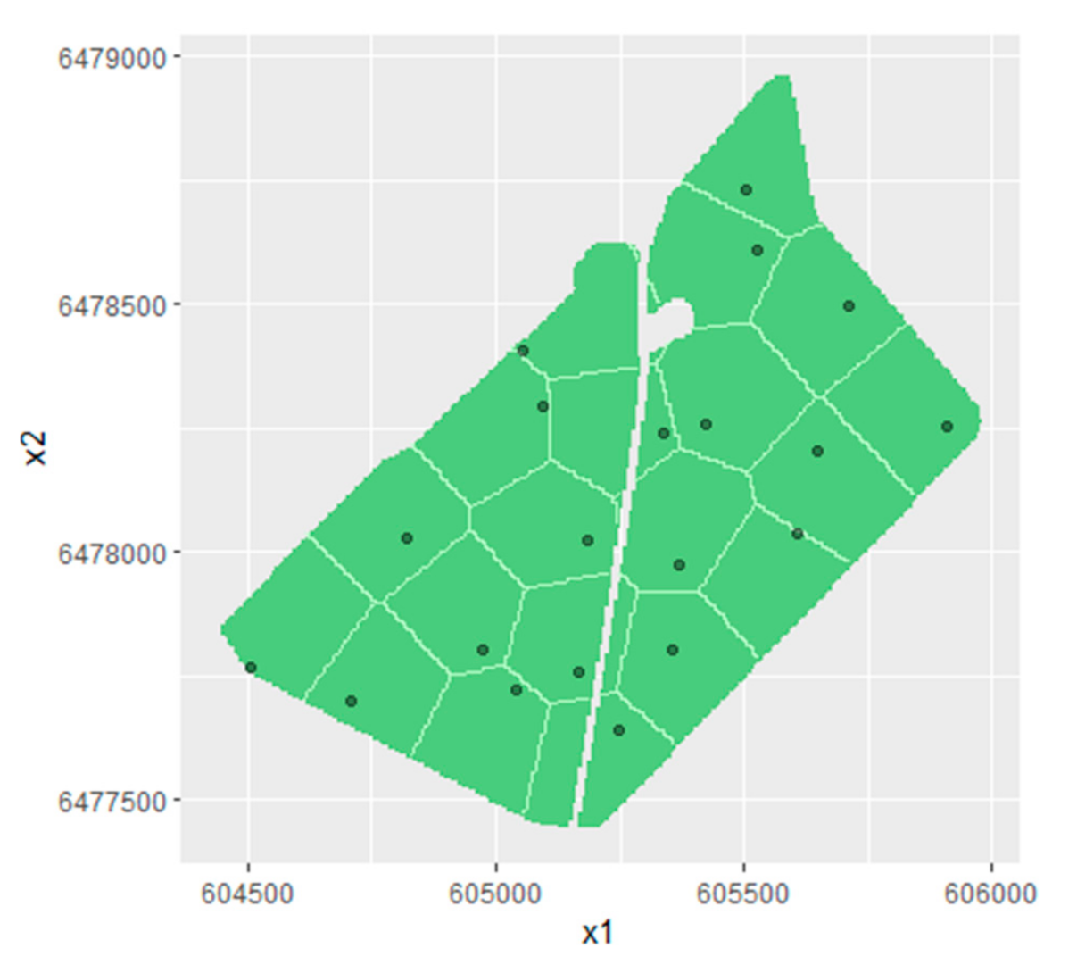
2.5.1. Random Transect Sampling

Random transect sampling was simulated to obtain a field average of soil conditions representing common agronomic practice for Australian agricultural fields (i.e., BR application). Transects were selected by randomising the start and end member location of the sampling transect along the field’s baselines (Figure 1), which were at 30 m parallel to the north-eastern and south-western field boundaries. The N samples were subsequently located at equidistant locations as a line between the defined end members to achieve each sampling density.

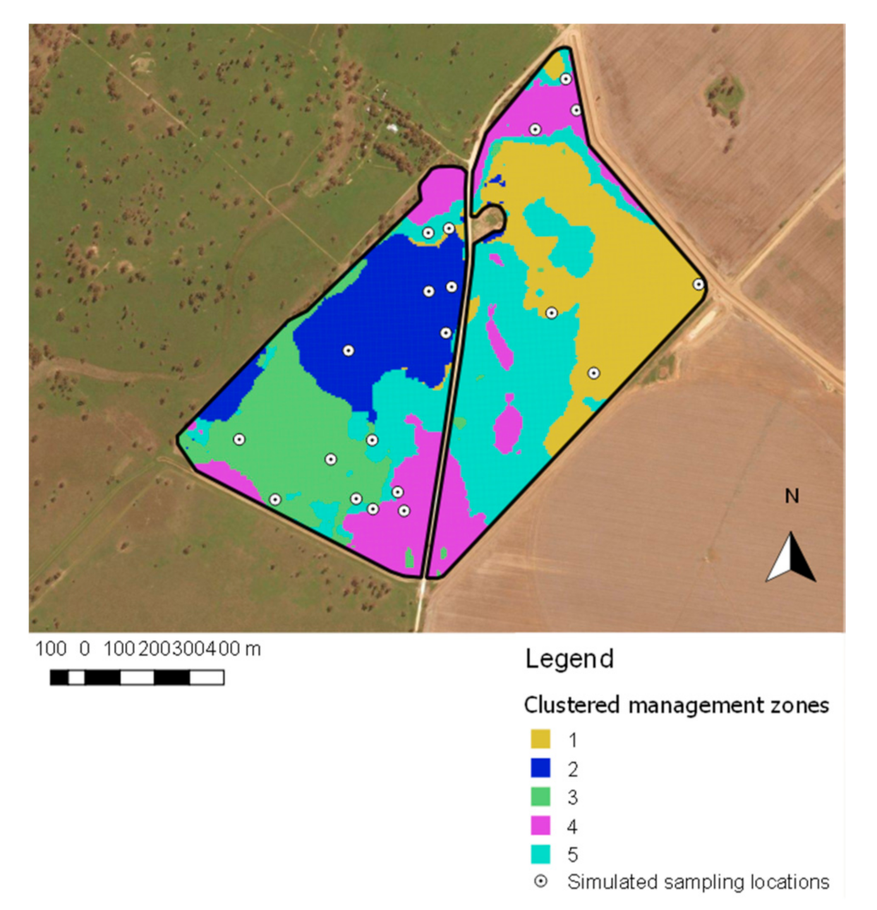
2.5.2. Management Zone Sampling

Spatial management zones were identified using k-means clustering of the covariate data, with five management zones selected (Figure 2). The number of management zones was consistent across all simulations (i.e., 5 zones), irrespective of sampling density. Whilst this approach is not preferred when developing DSMs, it was selected as the industry-standard zone-based variable-rate approach, which rarely sees >5 zones within a single field. From each management zone, N/5 sampling locations were randomly selected and used to calculate the mean of each soil property in each zone.

2.5.3. Ordinary Kriging

OK was implemented using automap package in the R programming environment [29] to fit the variogram models. A stratified random sampling procedure was employed to identify N sample locations using the k-means based spcosa package in the R programming environment [20]. Sampling locations were selected randomly within each strata (see Figure 3). Whilst it has been noted in the literature that variogram estimation for accurate kriging requires a minimum of 100 points [30], variograms were fitted at sampling densities as low as 10, to observe the effect poor variogram fitment has on final agronomic recommendations.

2.5.4. Regression Kriging

For each sampling density N, an RK model was fitted between the soil properties and the available covariates at N locations, with the residuals of the model subsequently being kriged across the geographic space and added to the predictions. The developed model for any given location x,y is given as:
S a = f EC a 1 , EC a 2 , EC a 3 , EC a 4 ,   Yield 2013 , Yield 2014 , Yield 2015 , Yield 2016 , elevation + e
where Sa is the soil attribute, ECa are the electrical conductivity readings at the 4 depth integrations, Yield represents crop yield measurements, elevation is the elevation above sea level at point (x, y) and e is the model error. The 9 features were reduced to 4 principal components, which explained 99% of the variability, for model training.
A conditioned Latin-hypercube approach [26] was adopted to select N training examples which insured the covariate feature space was appropriately represented in training (Figure 4). This was achieved by the application of the cLHS package in the R programming environment [31]. A mixed linear regression model was fitted to the environmental covariates for prediction of pH, ESP, BD and CEC.

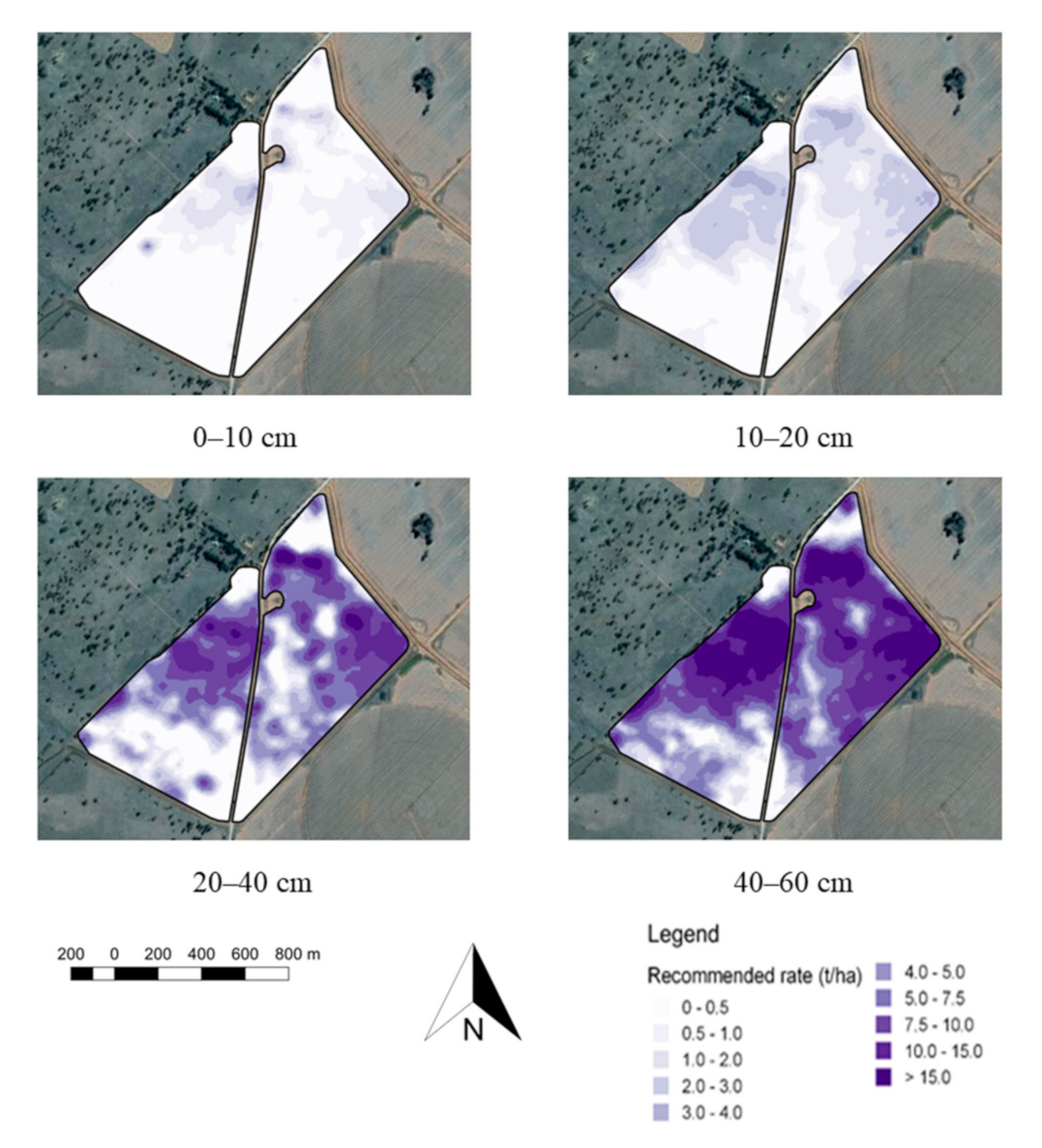
2.6. Amendment Requirement Calculations

The developed DSMs were used to calculate gypsum and lime recommendations for the site to investigate the agronomic and economic consequences of decisions made at various sampling densities. The widely accepted gypsum recommendation formula devised by Oster et al. [32] was adopted and is given as follows, for each depth layer:
G R = 0.086 × ρ b × d × C E C × E S P i E S P j
where ρb is the BDin Mg/m3, d is the depth to be treated in m, CEC is in mmolc/kg, ESPi and ESPj are the observed and target soil ESP. A value of ESPj = 3, as guided by Shainberg et al. [33], was used to provide a target benchmark for soil dispersion amelioration at all locations, with a calcium exchange efficiency factor of 75% [5]. Whilst it is not currently commercially possible to place gypsum at depth, future work will aim to demonstrate the potential benefits of subsoil amelioration in relation to the placement cost as a caveat to drive manufacturing of deep placement equipment. Demonstrating this benefit is outside the scope of the work presented here. The assumed baseline gypsum requirement—gypsum requirement calculated form the 300 core 60 × 60 m regular grid—is given in Table 2 and Figure 5.
Lime application rates were calculated using Equation (4), derived from [34]. This method is commonly adopted in lime recommendation tools in the Australian grains industry when only eCEC is available, see iLime (https://www.agric.wa.gov.au/apps/ilime). A conversion factor of 0.26 was adopted and the site’s texture was categorised as ‘clay’, with an application efficiency of 75% and a target pH of 7.
P u r e   l i m e   r e q u i r e m e n t   t / h a = T a r g e t   p H C u r r e n t   p H c o n v e r s i o n   f a c t o r × e f f i c i e n c y

3. Results

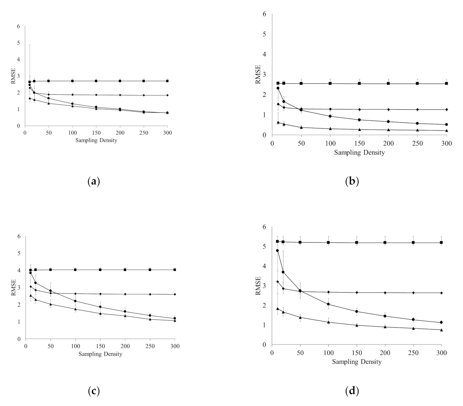
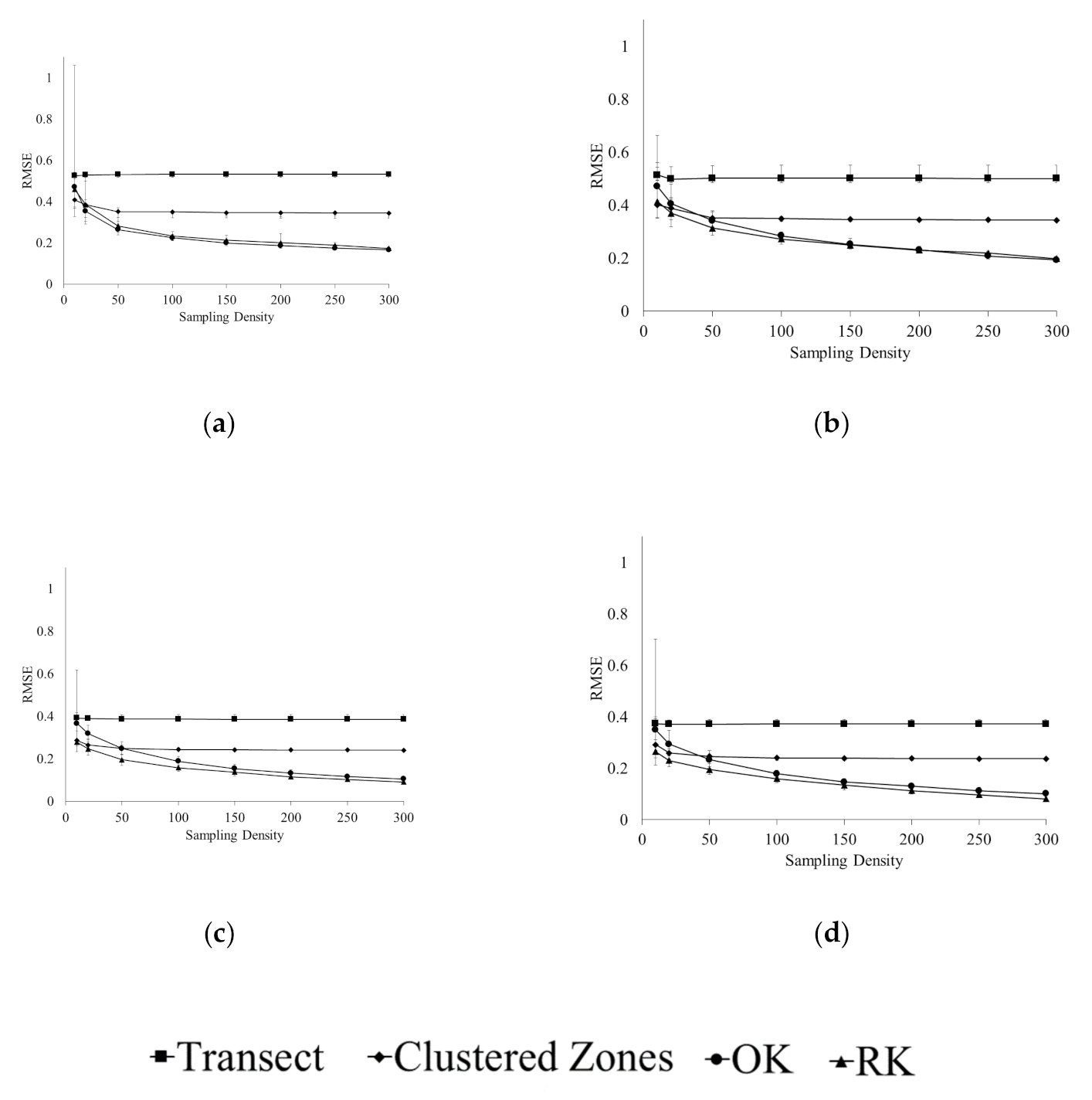
3.1. Accuracy of Spatial Prediction Methods

The ability to characterise and map soil pH and ESP at the investigation site for the four methods examined is summarised in Figure 6 and Figure 7, with multiple sampling densities presented. It is evident for all sampling densities that RK prevails over other methods in terms of characterising ESP at the investigation site, with OK providing similar results as RK for pH at <40 cm. Increases in sampling density do not appear to greatly change the spatial prediction errors of the random transect, however, are greatly influential on the predictive accuracy of clustering, OK and RK methods. For these three methods, the prediction accuracy greatly improves to a density of 100 samples, after which, only minimal improvements are achieved. Interestingly, superior predictions were achieved using a clustered approach over OK to a sampling density of approximately 50, after which OK prevails.
The accuracy of spatial predictions for OK is correlated with the degree of spatial variance present in the predicted layer. For soil pH predictions, accuracy generally increases with depth for all methods. This result is expected, as the spatial variance of soil pH also generally decreases with depth, with the exception of the 10–20 cm layer (Table 1). For ESP, however, spatial variance increases to depth, which explains the decreased prediction accuracy as depth increases.
The sensitivity of the models to random initialisation was tested and is represented by the error bars (2 standard deviations) presented in Figure 6 and Figure 7. At low sampling densities (i.e., ≤20), the RK and OK methods are most sensitive to sample selection, therefore expressing the largest degree of uncertainty. The uncertainty expressed by the RK at a sampling density of 10, however, is generally substantially greater than other methods, suggesting that the accuracy of regression kriging approaches are highly sensitive to calibration sample selection at low sampling densities. The prediction uncertainty decreases as the sampling density increases for all methods. The uncertainty of the transect method is consistent across all sampling densities and represents the greatest uncertainty at sampling densities ≥50.
The degree by which RK outperforms OK generally increases with depth. This can be explained by the increasing correlation between ESP and pH with the environmental covariates at the lower depth layers (Table 3).

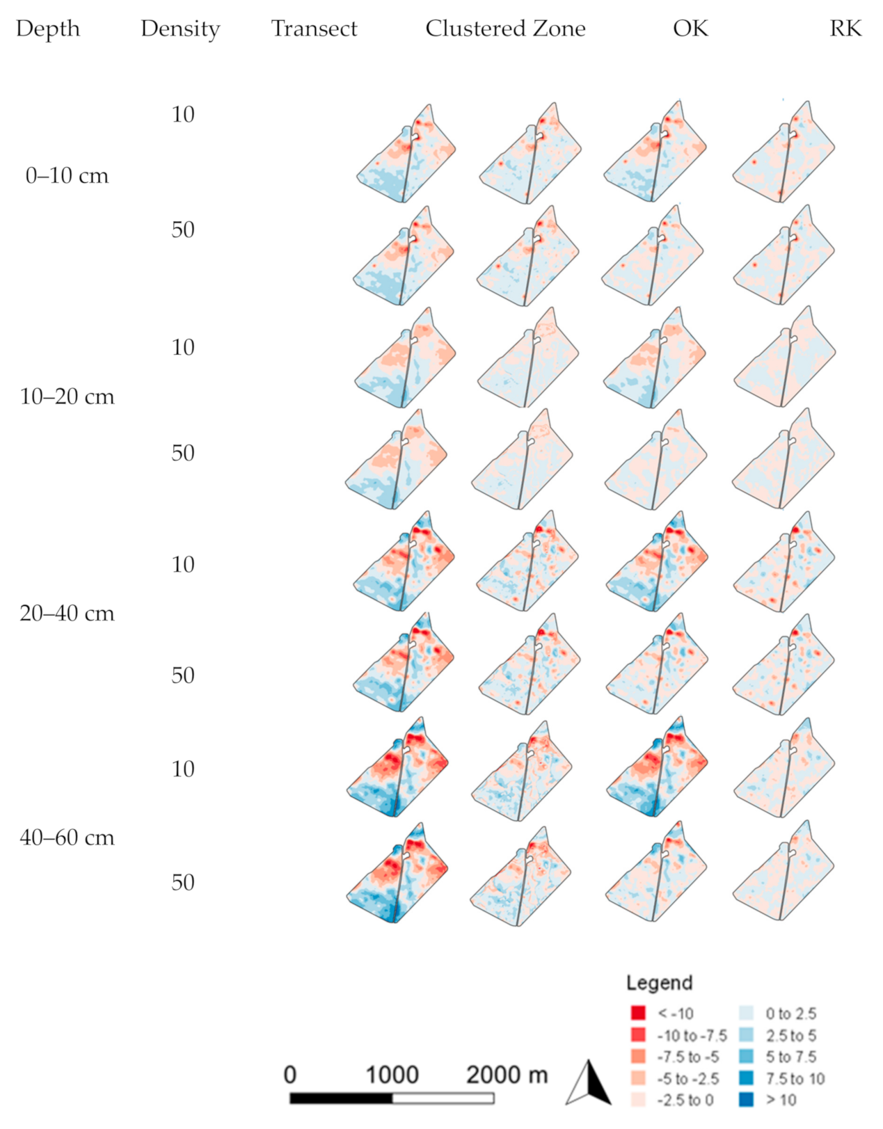
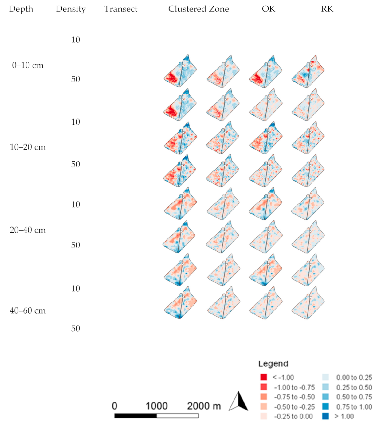
3.2. Spatial Prediction Errors

Prediction error maps for soil pH and ESP are displayed in Figure 8 and Figure 9, respectively. The spatial errors are of a higher magnitude at low sampling densities in the surface layer for pH, and the 40–60 cm layer for ESP. This agrees with the RMSE results of each prediction. The errors for both pH and ESP are spatially correlated, meaning that the areas of large error are generally spatially consistent across sampling methods and densities for a given depth. For example, this is seen in the 0–10 cm layer for soil pH, where all methods severely under-predicted values in the region to the south-west of the site, which correlates with zone 3 identified by k-means clustering. The spatial distribution of errors for the RK method, however, did not always agree with the other methods. This is seen in the 20–40 cm depth layer for ESP. Here, the higher magnitude errors are less spatially correlated and occur in smaller, more spatially irregular pockets in comparison to other methods.
Increases in sampling density did not greatly affect the spatial distribution of errors for the random transect and clustered zone methods for soil pH or ESP. This agrees with the RMSE findings in Figure 6 and Figure 7. For the OK and the RK method, however, the magnitude of error are considerably less and closer to the prediction as sampling density increased from 10 to 50 samples. These errors also become more spatially distributed.

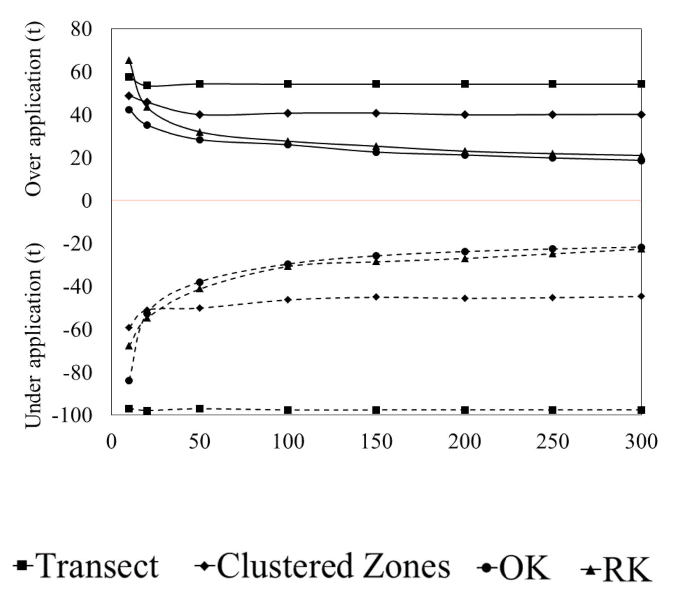
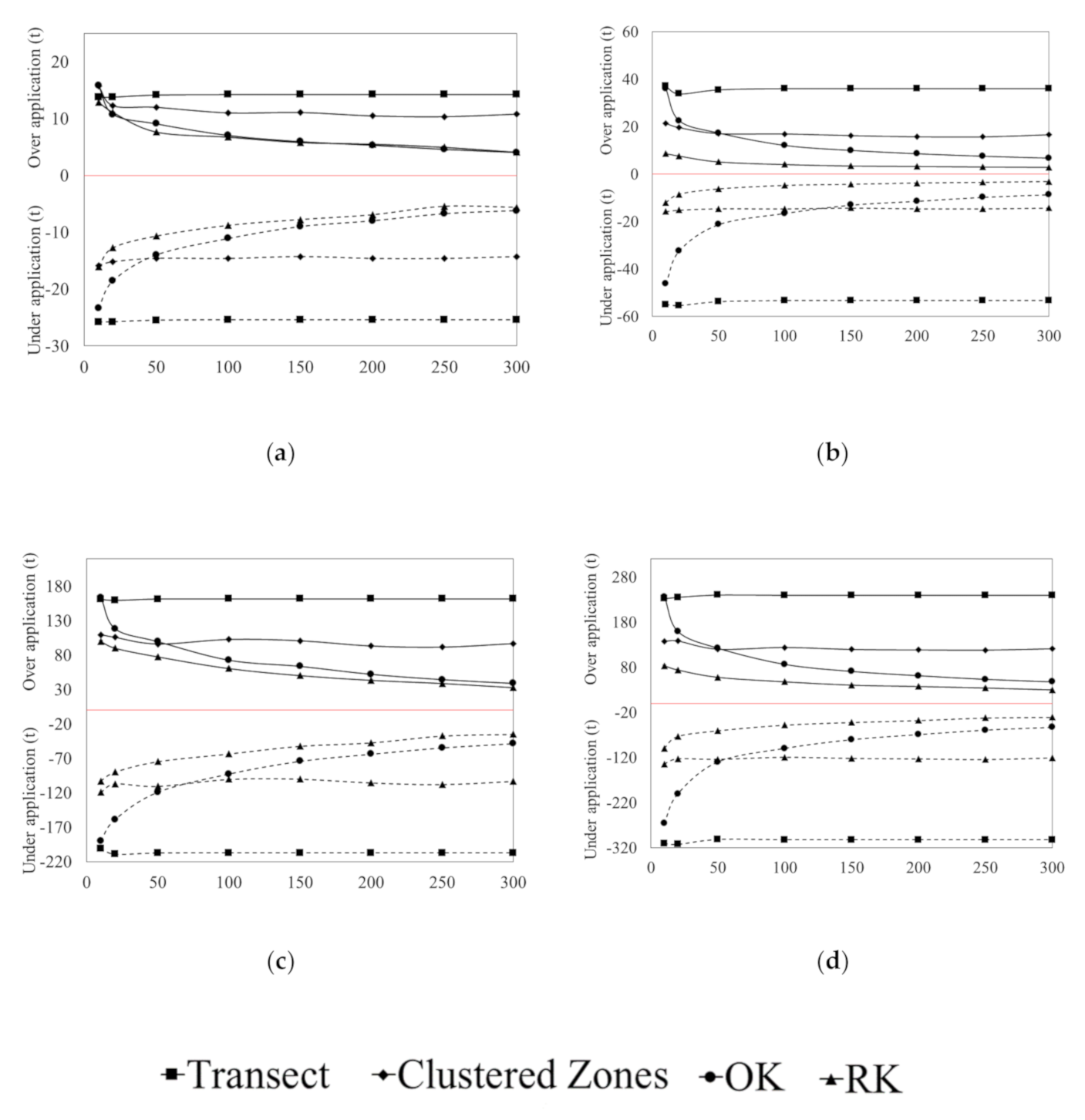
3.3. Error of Agronomic Recommendations

For each simulation of the four spatial prediction methods, gypsum and lime recommendations were calculated against the spatial resolution to observe the agronomic consequences of the prediction errors on individual soil properties (Figure 10 and Figure 11). These agronomic errors were estimated by calculating the net over- and under-application of the amendment for the eight sampling densities. The net error trend of gypsum and lime recommendations generally reflected that of the RMSE calculations, with error reducing as sampling density increased.
Error trends of gypsum and lime recommendations, based on the spatial predictions, generally agreed with that of the RMSE findings (Figure 10 and Figure 11). At all sampling densities, RK produced lower magnitude errors in under- and over-application of amendments. The magnitude of application error for the OK and RK decreased with increasing sampling densities, with errors remaining relatively consistent for the clustered zone and random transect methods. Interestingly, small changes in RMSE of ESP and pH predictions translated to large recommendation errors, in terms of both under- and over-application. This suggests that the accuracy of amendment recommendations are highly sensitive to small changes in spatial prediction performance.
Recommendations produced using the bulked transect sampling method were the most inaccurate for both gypsum and lime, with RK producing the best results. The OK method produced highly inaccurate recommendations at low sampling densities, however, this error rapidly decreased within the increasing sampling density. For both the RK and OK soil prediction methods, the errors greatly improved to a sampling density of 100 samples, after which minimal improvements were observed.

4. Discussion

4.1. Agronomic Consequences of Data Limited Recommendations

The bulked transect sampling method was used in this study to represent the standard agronomic practice. However, it is worth noting that this level of data collection over-estimates the level of sampling commonly undertaken for agronomic decision making [1,2]. The results conclusively established that bulked transect sampling was highly inaccurate in representing the site variability and subsequent site-specific gypsum and lime recommendations. By extension, this suggests that the current industry agricultural sampling strategies, which are likely more conservative than bulked transect sampling, would result in substantial errors pertaining to the resultant recommendations. Gypsum and lime recommendation errors were much greater for bulked transect sampling than that of other methods, with over-application magnitudes reaching in excess of 200 t in the 40–60 cm layer for gypsum and 50 t for lime in the 0–10 cm layer for the entire site. With gypsum application costs of approximately $110/t (transported and spread; Bennett et al. [4]), this error presents great economic significance.
Of potentially greater concern than the cost of over-application is the failure to spatially address the ESP and pH constraints, which would impact on yield potential. Much of the site was recommended an insufficient ameliorant quantity using the bulked transect method, with under-application being in the order of 25 t and 100 t for gypsum and lime respectively in the 0–10 cm surface layer, and 300t in the 40–60 cm subsurface layer for gypsum. This error is concerning, considering the level of investment that would be committed based on these recommendations. The long-term lost yield opportunity of this shortfall is likely an important consideration within a long-term amelioration strategy as the insufficient application may not actually result in yield increase, and the site-specific yield potential at the site cannot be realised. Therefore, using a bulked transect sampling approach for site-average recommendations is highly detrimental to the long term agronomic and economic performance of a farming unit, and should be avoided when providing recommendations.
Utilising a spatial sampling strategy to allow for continuous spatial prediction with OK without environmental covariates offers improved recommendations over the bulked transect method, however, this is minimal at low sampling densities (i.e., <20). When such covariates are available, a clustering approach to develop zone-based recommendations provides a more accurate recommendation over OK, at low sampling densities. This improvement is achieved by reducing the within-zone variance, using auxiliary information to identify ‘homogenous’ zones within a site that exhibit similar soil characteristics [35]. In doing so, it is assumed that soil properties and yield-limiting factors are consistent within each identified zone [36], and in this case, it is an incorrect assumption. Whilst the error introduced by this assumption is less than that of spatially averaging soil properties across an entire site, its magnitude is of great agronomic and economic significance, with over- and under-application of gypsum approaching 130 t in the 40–60 cm subsurface layer for the investigated site.
The ability for clustering to provide superior predictions over OK can only be achieved up to a certain sampling density, after which OK becomes superior (identified here at a sampling density ≈50). This is the result of the underlying assumption for clustering, which assumes that all soil properties are spatially correlated with each other and can be represented by the same set of global boundaries. Soil properties often vary independently of each other in both the x-y and z planes, meaning global boundaries cannot accurately characterise soil characteristics across multiple properties. This behaviour was observed at the investigation site (Figure 12), where surface pH varied independently of subsurface pH and both surface and subsurface ESP. Whilst under this assumption, the addition of environmental covariates provides improved predictions, these are limited by the inability to explain more subtle soil variance within each zone. Zone management, therefore, oversimplifies the detection of spatial variability by providing limited consideration towards the independent variability soil properties and level of spatial correlation that exists at the site.
Zone management is the currently accepted standard for variable rate recommendations for commercial precision agriculture [13,14,15,37]. However, for this site and application, it resulted in significant under- and over-application of soil amendment when compared to the RK approach using the sampling effort. The economic and agronomic effects of this are significant, due to both wasted resources and the failure to accurately address soil condition to overcome constraints. Agricultural technology is currently capable of applying soil amendment at a much finer scale than what is currently practiced in zone management, with some machines offering row-specific control (<1 m) (see John Deere ® RowCommandTM, Moline, IL, USA, www.deere.com) with the aid of sub 2 cm accurate RTK GNSS technology. Therefore, whilst zone-management offers improvements of BR applications, it’s data minimalist approach is currently limiting precision agriculture by failing to identify variation in soil conditions at the scale in which it can be managed using more advanced approaches.

4.2. Improving Recommendations through Advanced Spatial Prediction Methods with Increased Sampling Requirements

Spatial variable-rate recommendations can be improved significantly by adopting DSM methods that predict soil properties as a continuous function at fine scales. This was achieved for both the OK geostatistical method and RK model-based method for the investigation site. However, these improvements require substantial direct sampling in the case of OK (i.e., >50 samples), or acquisition of environmental covariates to reduce direct sampling in the case of RK. These DSM methods offer improvements over zone-based predictions by removing hard separating boundaries between changes in soil condition and expressing these as a continuous function [25].
The DSM methods were sensitive to increases in sampling density, with the majority of prediction improvement being achieved at 50 samples per 108 ha, from which minimal improvement is made thereafter. This suggests that the spatial variability at the site can be accurately characterised using a sampling density of one sample per 2 ha, and is practically meaningful at one sample per 5 ha. This density however does not guarantee an economically optimized site characterisation, as the cost of data acquisition is not considered against the economic benefit in terms of both the sampling cost and expected yield return. At low sampling densities, (i.e., <10), OK is highly inaccurate, suggesting that 20 samples is not sufficient to achieve an appropriate variogram fit. At this sampling density, however, it is not expected to achieve an appropriately fitted model to the data due to the inherent complexities within the soil system. Furthermore, OK is rarely applied at these low sampling densities due to the inaccuracies of fitting a variogram model [24], with Webster et al. [30] reporting that 100 samples are the absolute minimum required for an appropriate variogram fit. Whilst a data density of 20 or 50 samples may not be considered sufficient for OK or RK variogram fitting from a pedometric perspective, the agronomic error or these methods remains less than that of bulked transect and zone management methods at an equivalent density. Therefore, the context of the spatial prediction problem must be considered when determining acceptable sampling densities.
At all sampling densities, RK produced superior results over OK, as also found by Odeh et al. [21], Odeh et al. [22], Hengl et al. [23] and Bishop et al. [24]. However, it is worth noting that some bias may exist due to RK being adopted to create the baseline dataset, which comparisons were made against. The same issue was observed when repeating the analysis using OK for the baseline (results not shown here), with the subsequent results biasing OK as the better method. Future work should aim to investigate methods that offer unbiased spatial predictions of baseline datasets, such that OK and RK can be compared more fairly.
The spatial prediction accuracy of RK can also be improved by employing more sophisticated non-linear machine learning techniques that can detect complex relationships between soil properties and environmental variables. These have been applied in the literature using artificial neural networks [38,39,40], regression-trees [39,41,42], support vector machines [43,44] and artificial neural networks [45,46,47]. However, the data requirements of these methods are exponentially increased over linear methods, due to the absence of structural assumptions within the data that subsequently allows for higher complexity. In this study, these non-linear methods are not suitable for RK development given the data volume in comparison to the complexity of the problem (a data-limited environment), and may only offer improvements when the size of calibration sampling is large.

4.3. The Effect of Sample Selection on Prediction Uncertainty

Each of the four methods investigated employs a random initialisation of search parameters that identify the selection of samples used in the spatial predictions. A level of uncertainty therefore exists for each method. Uncertainty generally decreases with increased sampling density, as a greater percentage of the total population is accounted for. Whilst the superior mean predictions were achieved with RK across all sampling densities, the method’s uncertainty at a density of 10 was greatest, suggesting a high degree of sensitivity to the random initialisation of calibration sample selection. Whilst the cLHS technique employed to select calibration samples ensures appropriate distribution within the feature space, it cannot guarantee that the selected samples are representative of the relationships that exist between the environmental covariates and soil properties. Model calibration is therefore highly biased towards these samples. This bias can only be reduced by increasing sampling requirements. The magnitude of this uncertainty suggests that RK methods should not be attempted at sampling densities <20, although this is dependent on the inherent variability that exists within the site and the ability of exploratory variables to represent all of the variability.
The assumed industry-standard method of using a bulked transect was shown to be highly sensitive to the selection of the transect from which samples are taken. Using this method, gypsum recommendations were up to 482% incorrect in the surface layer and 32% incorrect in the 40–60 cm subsurface layer. In practice, the transect is rarely truly randomised, and is instead often selected to simply span the diagonal length of the field, with limited attempt to appropriately represent the inherent variability of the site. This presents a large agronomic concern, as the soil amendment advice that is provided is largely influenced by how the transect was selected. Furthermore, while zonal management provides an improvement on this, it has been shown here that by using the same number of samples within the field, a much more improved outcome can be achieved using advanced techniques such as RK. This is a significant opportunity for agriculture, as it requires no further expense in sampling, but delivers improved predictions with higher uncertainty. This work has presented a detailed investigation for a single site, and we acknowledge that there are limitations related to this. Specifically, the results obtained should not be expected to directly transfer to new sites. However, this work provides a valuable discussion of the considerations for data density and should be used over a range of new sites in order to confirm the practically useful recommendation of one sample in every 5 ha, as well as the accurate recommendation of one sample in every 2 ha, for the spatially continuous RK and cLHS methods.

5. Conclusions

Improved understanding of how the variability of agricultural soils influences the accuracy of variable-rate soil amelioration advice is required to drive on-farm profitability, with consideration toward to social responsibility of management. Furthermore, it must be understood how this advice is influenced by different sampling techniques employed at various levels of soil sampling investment. The results in this study have shown the agronomic advice based on the widely adopted, bulk transect sampling method for blanket rate application of soil amendment is largely inaccurate, leading to potentially large under- and over- applications of amendments at significant cost to the grower (either as yield penalty or unnecessary application). Using this approach, application of gypsum and lime is frequently misapplied to the spatial areas where it is most required, with the total over- and under- application tonnages within a single field being substantial (i.e., >320 t and 560 t respectively for a 108 ha field for treatment to 60 cm). Transect sampling for blanket-rate application should be avoided for soil amelioration recommendations
The most accurate applications of gypsum and lime were achieved using a variable-rate approach, based on an RK spatial prediction method. This was achieved over all the sampling densities. Whilst traditionally it was been recommended that neither RK or OK should be applied at such low densities [30], we have shown here the importance of assessing prediction errors practically by evaluating the accuracy of resulting land management decisions to determine acceptable sampling requirements. Whilst it is important to investigate the statistical cost of reduced sampling density, it is also pertinent to investigate the economic cost of land management decisions at such densities.
It is important to note that RK may only provide superior results when a correlation exists between the environmental covariates and the individual soil property. Therefore, the environmental correlation between the auxiliary information and predicted soil attributes should be considered prior to the deployment of this method. Hence, where this correlation is poor, or at worst, unknown, both OK and RK methods should be considered simultaneously in providing spatial agronomic advice, for example, using probability sampling validation [48]. Furthermore, the economic cost of acquiring such covariates must also be considered against the relative increased spatial predictions and subsequent decisions.
Sampling density was shown to be highly influential on the recommendation advice for OK and RK methods, however, did not contribute to large changes in the error for transect sampling or zone management. Spatial prediction and recommendation accuracies greatly improved to a sampling density of 50 for OK and RK, with minor improvements being achieved thereafter. Selecting the most optimal sampling density requires further consideration towards the economics of increased data collection and its effects on crop performance due to improved spatial agronomic advice for soil amelioration.

Author Contributions

Investigation S.D.R.; Writing—original draft, J.M.B.; Writing—review & editing, C.R.L. and T.F.A.B. All authors have read and agreed to the published version of the manuscript.

Funding

This research was funded by Grains Research and Development Corporation: GRS11002.

Acknowledgments

The work presented here was generously funded by Grains Research and Development Corporation (GRDC) through a GRS scholarship, and further supported by the University of Southern Queensland.

Conflicts of Interest

The authors declare no conflict of interest.

References

  1. Lobry de Bruyn, L.; Andrews, S. Are Australian and United States farmers using soil information for soil health management? Sustainability 2016, 8, 304. [Google Scholar] [CrossRef] [Green Version]
  2. Bennett, J.M.; Cattle, S. Adoption of soil health improvement strategies by Australian farmers: I. Attitudes, management and extension implications. J. Agric. Educ. Ext. 2013, 19, 407–426. [Google Scholar] [CrossRef]
  3. Bennett, J.M.; Cattle, S. Adoption of soil health improvement strategies by Australian farmers: II. Impediments and incentives. J. Agric. Educ. Ext. 2014, 20, 107–131. [Google Scholar] [CrossRef]
  4. Bennett, J.M.; Cattle, S.; Singh, B. The efficacy of lime, gypsum and their combination to ameliorate sodicity in irrigated cropping soils in the Lachlan Valley of New South Wales. Arid Land Res. Manag. 2015, 29, 17–40. [Google Scholar] [CrossRef]
  5. Bennett, J.M.; Marchuk, A.; Raine, S.R.; Dalzell, S.A.; Macfarlane, D.C. Managing land application of coal seam water: A field study of land amendment irrigation using saline-sodic and alkaline water on a Red Vertisol. J. Environ. Manag. 2016, 184, 178–185. [Google Scholar] [CrossRef]
  6. Heath, R. Editorial to John Ralph Essay Competition 2018: Should society determine the right to farm? Farm Policy J. 2018, 15, 2–3. [Google Scholar]
  7. Lush, D. Should society determine the right to farm? Farm Policy J. 2018, 15, 4. [Google Scholar]
  8. Bennett, J.M.; Bennett, J.M.; McBratney, A.; Field, D.; Kidd, D.; Stockmann, U.; Liddicoat, C.; Grover, S. Soil Security for Australia. Sustainability 2019, 11, 3416. [Google Scholar] [CrossRef] [Green Version]
  9. De Gruijter, J.J. Numerical Classification of Soils and Its Application in Survey; Pudoc: Wageningen, The Netherlands, 1977. [Google Scholar]
  10. Boydell, B.; McBratney, A. Identifying potential within-field management zones from cotton-yield estimates. Precis. Agric. 2002, 3, 9–23. [Google Scholar] [CrossRef]
  11. Fu, Q.; Wang, Z.; Jiang, Q. Delineating soil nutrient management zones based on fuzzy clustering optimized by PSO. Math. Comput. Model. 2010, 51, 1299–1305. [Google Scholar] [CrossRef]
  12. Taylor, J.; McBratney, A.; Whelan, B. Establishing management classes for broadacre agricultural production. Agron. J. 2007, 99, 1366–1376. [Google Scholar] [CrossRef]
  13. Li, Y.; Shi, Z.; Li, F.; Li, H.-Y. Delineation of site-specific management zones using fuzzy clustering analysis in a coastal saline land. Comput. Electron. Agric. 2007, 56, 174–186. [Google Scholar] [CrossRef]
  14. McBratney, A.; Whelan, B.; Ancev, T.; Bouma, J. Future directions of precision agriculture. Precis. Agric. 2005, 6, 7–23. [Google Scholar] [CrossRef]
  15. Robertson, M.J.; Llewellyn, R.S.; Mandel, R.; Lawes, R.; Bramley, R.G.V.; Swift, L.; Metz, N.; O’Callaghan, C. Adoption of variable rate fertiliser application in the Australian grains industry: Status, issues and prospects. Precis. Agric. 2012, 13, 181–199. [Google Scholar] [CrossRef]
  16. Burgess, T.; Webster, R. Optimal interpolation and isarithmic mapping of soil properties: I. The semivariogram and punctual kriging. J. Soil Sci. 1980, 31, 315–331. [Google Scholar] [CrossRef]
  17. Brus, D.J.; Heuvelink, G.B. Optimization of sample patterns for universal kriging of environmental variables. Geoderma 2007, 138, 86–95. [Google Scholar] [CrossRef]
  18. Heuvelink, G.B.; Brus, D.J.; de Gruijter, J.J. Optimization of sample configurations for digital mapping of soil properties with universal kriging. Dev. Soil Sci. 2006, 31, 137–151. [Google Scholar]
  19. Vašát, R.; Heuvelink, G.; Borůvka, L. Sampling design optimization for multivariate soil mapping. Geoderma 2010, 155, 147–153. [Google Scholar] [CrossRef]
  20. Walvoort, D.J.; Brus, D.; De Gruijter, J. An R package for spatial coverage sampling and random sampling from compact geographical strata by k-means. Comput. Geosci. 2010, 36, 1261–1267. [Google Scholar] [CrossRef]
  21. Odeh, I.; McBratney, A.; Chittleborough, D. Spatial prediction of soil properties from landform attributes derived from a digital elevation model. Geoderma 1994, 63, 197–214. [Google Scholar] [CrossRef]
  22. Odeh, I.O.; McBratney, A.; Chittleborough, D. Further results on prediction of soil properties from terrain attributes: Heterotopic cokriging and regression-kriging. Geoderma 1995, 67, 215–226. [Google Scholar] [CrossRef]
  23. Hengl, T.; Heuvelink, G.B.; Stein, A. A generic framework for spatial prediction of soil variables based on regression-kriging. Geoderma 2004, 120, 75–93. [Google Scholar] [CrossRef] [Green Version]
  24. Bishop, T.; McBratney, A. A comparison of prediction methods for the creation of field-extent soil property maps. Geoderma 2001, 103, 149–160. [Google Scholar] [CrossRef]
  25. McBratney, A.; Mendonça Santos, M.L.; Minasny, B. On digital soil mapping. Geoderma 2003, 117, 3–52. [Google Scholar] [CrossRef]
  26. Minasny, B.; McBratney, A.B. A conditioned Latin hypercube method for sampling in the presence of ancillary information. Comput. Geosci. 2006, 32, 1378–1388. [Google Scholar] [CrossRef]
  27. IUSS Working Group WRB. World Reference Base for Soil Resources 2014, Update 2015: International Soil Classification System for Naming Soils and Creating Legends for Soil Maps; FAO: Rome, Italy, 2015; p. 192. [Google Scholar]
  28. Rayment, G.E.; Lyons, D.J. Soil Chemical Methods: Australasia; CSIRO Publishing: Collingwood, Australia, 2011; Volume 3. [Google Scholar]
  29. Hiemstra, P.; Hiemstra, M.P. Package ‘Automap’; Carnegie-Mellon University Institute for Software Research: Pittsburgh, PA, USA, 2013; Volume 105, p. 10. [Google Scholar]
  30. Webster, R.; Oliver, M.A. Sample adequately to estimate variograms of soil properties. J. Soil Sci. 1992, 43, 177–192. [Google Scholar] [CrossRef]
  31. Minasny, B.; McBratney, A. Latin hypercube sampling as a tool for digital soil mapping. Dev. Soil Sci. 2006, 31, 153–606. [Google Scholar]
  32. Roudier, P.; Beaudette, D.; Hewitt, A.A. A conditioned Latin hypercube sampling algorithm incorporating operational constraints. In Digital Soil Assessments and Beyond: Proceedings of the 5th Global Workshop on Digital Soil Mapping, Sydney, Australia, 10–13 April 2012; Taylor & Francis: Sydney, Australia, 2012; pp. 227–231. [Google Scholar]
  33. Oster, J.; Jayawardane, N. Agricultural Management of Sodic Soils, In Sodic Soil: Distribution, Management and Envrionmental Consequences; Oxford University Press: New York, NY, USA, 1998. [Google Scholar]
  34. Shainberg, I.; Rhoades, J.; Prather, R. Effect of Low Electrolyte Concentration on Clay Dispersion and Hydraulic Conductivity of a Sodic Soil 1. Soil Sci. Soc. Am. J. 1981, 45, 273–277. [Google Scholar] [CrossRef]
  35. Helyar, K.R.; Porter, W. Soil acidification, its measurement and the processes involved. In Soil Acidity and Plant Growth; Academic Press: Marrickvlle, Australia, 1989; pp. 61–102. [Google Scholar]
  36. Doerge, T. Defining management zones for precision farming. Crop Insights 1999, 8, 1–5. [Google Scholar]
  37. Whelan, B.; McBratney, A. Definition and interpretation of potential management zones in Australia. In Proceedings of the 11th Australian Agronomy Conference, Geelong, VIC, Australia, 2–6 February 2003. [Google Scholar]
  38. Florinsky, I.V.; Eilers, R.G.; Manning, G.R.; Fuller, L.G. Prediction of soil properties by digital terrain modelling. Environ. Model. Softw. 2002, 17, 295–311. [Google Scholar] [CrossRef]
  39. McKenzie, N.J.; Ryan, P.J. Spatial prediction of soil properties using environmental correlation. Geoderma 1999, 89, 67–94. [Google Scholar] [CrossRef]
  40. Minasny, B.; McBratney, A. Conditioned Latin hypercube sampling for calibrating soil sensor data to soil properties. In Proximal Soil Sensing; Springer: Dordrecht, The Netherlands, 2010; pp. 111–119. [Google Scholar]
  41. Henderson, B.L.; Bui, E.N.; Moran, C.J.; Simon, D.A.P. Australia-wide predictions of soil properties using decision trees. Geoderma 2005, 124, 383–398. [Google Scholar] [CrossRef]
  42. Lacoste, M.; Minasny, B.; McBratney, D.; Michot, D.; Viaud, V.; Walter, C. High resolution 3D mapping of soil organic carbon in a heterogeneous agricultural landscape. Geoderma 2014, 213, 296–311. [Google Scholar] [CrossRef]
  43. Ballabio, C. Spatial prediction of soil properties in temperate mountain regions using support vector regression. Geoderma 2009, 151, 338–350. [Google Scholar] [CrossRef]
  44. Were, K.; Bui, D.T.; Dick, Ø.B.; Singh, B.R. A comparative assessment of support vector regression, artificial neural networks, and random forests for predicting and mapping soil organic carbon stocks across an Afromontane landscape. Ecol. Indic. 2015, 52, 394–403. [Google Scholar] [CrossRef]
  45. Dai, X.; Huo, Z.; Wang, H. Simulation for response of crop yield to soil moisture and salinity with artificial neural network. Field Crops Res. 2011, 121, 441–449. [Google Scholar] [CrossRef]
  46. Behrens, T.; Förster, H.; Scholten, T.; Steinrücken, U.; Spies, E.D.; Goldschmitt, M. Digital Soil Mapping using Artificial Neural Networks. J. Plant Nutr. Soil Sci. 2005, 168, 21–33. [Google Scholar] [CrossRef]
  47. Chang, D.-H.; Islam, S. Estimation of soil physical properties using remote sensing and artificial neural network. Remote Sens. Environ. 2000, 74, 534–544. [Google Scholar] [CrossRef]
  48. Brus, D.; Kempen, B.; Heuvelink, G. Sampling for validation of digital soil maps. Eur. J. Soil Sci. 2011, 62, 394–407. [Google Scholar] [CrossRef]
Figure 1. Example of one simulation of random transect selection with N = 20 samples.
Agronomy 10 01676 g001
Figure 2. Spatial clusters identified using k-means clustering based on 9 environmental covariates. Sampling locations are shown for one simulation at sampling density N = 20.
Agronomy 10 01676 g002
Figure 3. Example of site stratification for random selection of N = 20 samples.
Agronomy 10 01676 g003
Figure 4. Example of sample site selection using cLHS for one simulation of N = 20 sampling density.
Agronomy 10 01676 g004
Figure 5. Actual spatial gypsum recommendation based on observed samples for the 4 depth increments.
Agronomy 10 01676 g005
Figure 6. Mean RMSE of soil pH predictions over 10 simulations at depths 0–10 cm (a), 10–20 cm (b), 20–40 cm (c) 40–60 cm (d) for the 4 sampling methods investigated. Error bars represent 2 standard deviations of RMSE predictions range for 50 simulations for each sampling density (x samples/108 ha).
Agronomy 10 01676 g006
Figure 7. Mean RMSE of soil ESP predictions over 10 simulations at depths 0–10 cm (a), 10–20 cm (b), 20–40 cm (c) 40–60 cm (d) for the 4 sampling methods investigated. Error bars represent 2 standard deviations of the RMSE range for 50 simulations for each sampling density (x samples/108 ha).
Agronomy 10 01676 g007
Figure 8. Mean prediction error maps of the 4 methods investigated for soil pH at 60 cm. Error maps shown for sampling densities N = 10 and 50. Red shades represent under prediction whilst blue shades represent over prediction.
Agronomy 10 01676 g008
Figure 9. Mean prediction error maps of the 4 methods investigated for soil ESP at 60 cm. Error maps shown for sampling densities N = 10 and 50. Red shades represent under prediction whilst blue shades represent over prediction.
Agronomy 10 01676 g009
Figure 10. Summary of gypsum application recommendations of 4 depth increments of 0–10 cm (a), 10–20 cm (b), 20–40 cm (c) 40–60 cm (d), based on the spatial predictions of the 4 methods investigated over various sampling densities. Solid and dashed lines represent the over and under application of gypsum for the site respectively (x samples/108 ha).
Agronomy 10 01676 g010
Figure 11. Summary of lime application recommendations of the 0–10 cm surface layer based on the spatial predictions of the 4 methods investigated over various sampling densities. Solid and dashed lines represent the over and under application of gypsum for the site respectively (x samples/108 ha).
Agronomy 10 01676 g011
Figure 12. Measured soil pH and ESP maps for the investigation site within the 0–10 cm and 40–60 cm depth layers.
Agronomy 10 01676 g012aAgronomy 10 01676 g012b
Table 1. Summary of directly measured soil attributes for all depth increments.
0–10 cm10–20 cm20–40 cm40–60 cm
MinMaxAverageSDMinMaxAverageSDMinMaxAverageSDMinMaxAverageSD
pH5.279.156.580.645.989.237.520.686.559.458.230.575.989.658.720.56
BD1.181.831.470.111.371.841.610.081.011.851.640.081.11.911.680.07
CEC5.7838.2816.556.397.6439.2123.316.1610.0766.528.245.4611.0541.9829.574.53
ESP0.0320.864.013.170.1326.215.323.750.0530.337.364.690.143410.485.9
Table 2. Summary of gypsum recommendation for the site at all depths.
DepthTotal (t)
0–10 cm36.5
10–20 cm109.7
20–40 cm517.05
40–60 cm952.85
Table 3. Correlation coefficients for environmental covariates and soil properties used in the development of RK. Subscript 1–4 represents depth layers 0–10 cm, 10–20 cm, 20–40 cm and 40–60 cm, respectively. Highlighted cells contain correlation coefficients ≥0.5.
pH1pH2pH3pH4ESP1ESP2ESP3ESP4
2013 Yield0.470.480.370.270.200.270.230.33
2014 Yield0.410.250.130.030.050.020.040.08
2015 Yield0.320.260.180.010.180.130.130.17
2016 Yield0.390.220.060.160.160.140.140.19
0–25 cm ECa0.070.360.490.490.580.630.680.78
0–75 cm ECa0.040.330.490.510.570.630.680.78
0–125 cm ECa0.070.350.500.520.550.610.660.77
0–275 cm ECa0.030.310.490.520.520.590.640.74
Elevation0.520.270.080.240.440.360.400.41
Publisher’s Note: MDPI stays neutral with regard to jurisdictional claims in published maps and institutional affiliations.

