Article

Near Real-Time Biophysical Rice (Oryza sativa L.) Yield Estimation to Support Crop Insurance Implementation in India

1
Potsdam Institute for Climate Impact Research (PIK), Member of the Leibniz Association, 14473 Potsdam, Germany
2
Agroecosystem Analysis and Modelling, Faculty of Organic Agricultural Sciences, University of Kassel, 37213 Kassel, Germany
*
Author to whom correspondence should be addressed.
Agronomy 2020, 10(11), 1674; https://doi.org/10.3390/agronomy10111674
Submission received: 23 September 2020 / Revised: 21 October 2020 / Accepted: 28 October 2020 / Published: 29 October 2020

Abstract

:
Immediate yield loss information is required to trigger crop insurance payouts, which are important to secure agricultural income stability for millions of smallholder farmers. Techniques for monitoring crop growth in real-time and at 5 km spatial resolution may also aid in designing price interventions or storage strategies for domestic production. In India, the current government-backed PMFBY (Pradhan Mantri Fasal Bima Yojana) insurance scheme is seeking such technologies to enable cost-efficient insurance premiums for Indian farmers. In this study, we used the Decision Support System for Agrotechnology Transfer (DSSAT) to estimate yield and yield anomalies at 5 km spatial resolution for Kharif rice (Oryza sativa L.) over India between 2001 and 2017. We calibrated the model using publicly available data: namely, gridded weather data, nutrient applications, sowing dates, crop mask, irrigation information, and genetic coefficients of staple varieties. The model performance over the model calibration years (2001–2015) was exceptionally good, with 13 of 15 years achieving more than 0.7 correlation coefficient (r), and more than half of the years with above 0.75 correlation with observed yields. Around 52% (67%) of the districts obtained a relative Root Mean Square Error (rRMSE) of less than 20% (25%) after calibration in the major rice-growing districts (>25% area under cultivation). An out-of-sample validation of the calibrated model in Kharif seasons 2016 and 2017 resulted in differences between state-wise observed and simulated yield anomalies from –16% to 20%. Overall, the good ability of the model in the simulations of rice yield indicates that the model is applicable in selected states of India, and its outputs are useful as a yield loss assessment index for the crop insurance scheme PMFBY.

1. Introduction

In India, around 44% of the country’s population relies directly or indirectly on agriculture, and more than 75% of the country’s farmers are smallholders with insecure access to food and income [1,2]. Many of these smallholder farmers produce rice, which is one of the major staple crops, and it is cultivated on about 44 million hectares out of 158 million hectares (globally), producing 105 million metric tons, which is over a quarter of the global rice production [3]. In order to ensure the nation’s food security and socio-economic development, a stable farmer’s income is obligatory. Risk transfer through crop insurance is one way to stabilize farmers’ incomes in areas with inter-annual weather and yield variability. Realizing this, crop insurance started in India in 1972 [1]. Over the years, several schemes were developed to cover crop yield losses by insurance payouts. However, these schemes were not widely adopted due to late payouts, lack of transparency, high premium costs because of high cost for sending claim adjusters to the fields, inefficient Crop Cutting Experiments (CCE), and coarse non-representative sampling. The current crop insurance scheme, Pradhan Mantri Fasal Bima Yojana (PMFBY), was established in 2016 with operational guidelines to promote the use of technologies and other related solutions to overcome these issues. PMFBY guidelines require geospatial biophysical crop modeling (0.05°) as one of the primary techniques that should be used to settle insurance claims after calibration and validation in addition to Crop Cutting Experiments (CCE) [4]. In this scheme, biophysical crop models could alternatively serve as justification for payout decisions if CCEs produce implausible results, contain outliers, or as justification for the CCEs. The results of these crop models could also be useful in developing climate-smart practices and other related applications for risk reduction apart from crop insurances.
Various biophysical crop simulation models, such as the Decision Support System for Agrotechnology Transfer (DSSAT), web-based SImulation Model for RIce-Weather relations (SIMRIW), and GIS-based Erosion Productivity Impact Calculator (GEPIC), have been used in studies on climate change and weather impacts, adaptation strategies, and yield estimation in India [5,6,7,8,9]. However, these studies were conducted on aggregated regions and a rather coarse resolution, in particular for the highly heterogeneous agricultural landscape in India, and mostly homogeneous management options. As such, these are not applicable to crop insurance questions on a 5km spatial regional scale as required by the PMFBY. There are also various global scale studies conducted in terms of yield estimation, but these are equally not pertinent in regional yield loss compensation [10,11,12,13,14,15]. In addition, there some remote sensing-based yield estimation using linear and non-linear approaches that are applicable at regional and local scales [16,17], which lacks temporal resolution and non-applicable to heterogeneous agricultural landscape. In addition, there are a few studies up to date that integrate remote sensing and biophysical models to obtain very-high-resolution yield information. However, these studies are currently restricted to small regions [18,19,20] due to the large size of India. Therefore, to support a higher penetration of crop insurance, regional geospatial (5 km) real-time crop modeling for the whole of India is needed. The implementation of better resolution (5 km) biophysical crop modeling in India is challenging due to highly diversified management practices and climatic variance. Nevertheless, new opportunities have arisen with large-scale, publicly available data for agricultural assessments [21]. With 5 km spatial resolution real-time weather data, monitoring crop growth and production through biophysical crop modeling can be more accurate, efficient, and also resource-saving [22]. In this study, we make use of these new developments by estimating yield anomalies using the DSSAT biophysical crop model for Kharif rice in India. These outputs can be helpful to gauge near real-time (two weeks after the harvest) yield losses and thus to settle crop insurance claims in a transparent scientific way over a large scale and at a better resolution. This technology eventually can support quick compensation for crop losses, enabling a more stable income of farmers. Therefore, the aim of this study is to develop a crop modelling framework for insurance payouts in India for Kharif rice. Specifically we sought to (i) model rice yield at 5 km resolution, (ii) to provide a method for real-time in-season crop monitoring for immediate payouts and (iii) to use open-source data (gridded secondary crop model inputs), which can be applied to other parts of the world. These three contributions could significantly support the PMFBY scheme being operational.

2. Materials and Methods
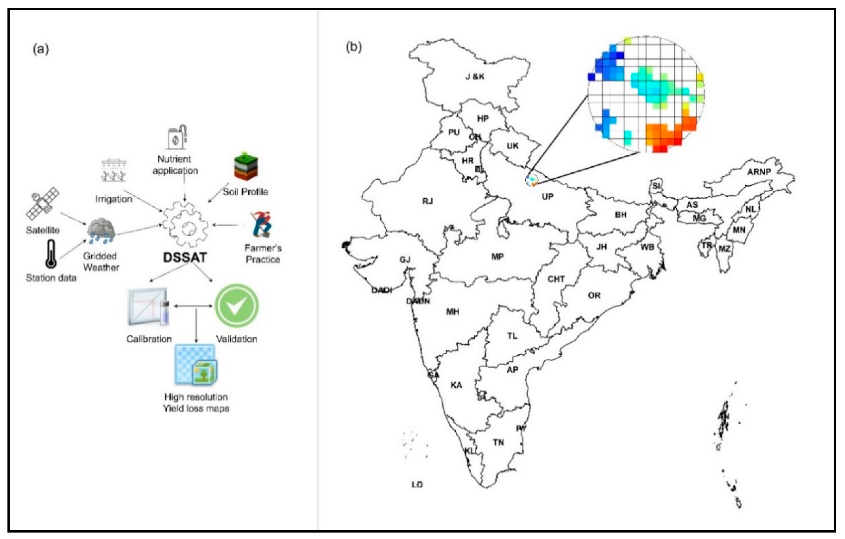
2.1. Crop Model

Biophysical crop simulation models simultaneously incorporate interacting soil, plant, field inputs, and weather information. In this study, we used DSSAT [23,24], a widely used process-based crop simulation model that simulates crop growth as a function of the soil–plant–atmosphere dynamics. The model requires daily weather data, soil surface and profile information, detailed crop management information, and genetic coefficients of variety as inputs to simulate crop growth. DSSAT calculates plant and soil water, nitrogen, phosphorus, and carbon balances, as well as the vegetative and reproductive development of crops at the daily temporal interval. For this study, DSSAT “seasonal” (i.e., multiple years run with the same initial conditions) simulations are involved in estimating yield anomalies for the Kharif rice season from 2001 to 2017 at 5 km spatial resolution (0.05°) in India. India consists of 36 states, 684 districts, and 5969 sub-districts (2015 census). However, as rice is not planted in all parts of India and observed data were not available for all rice cultivating areas, only 372 Districts from 19 States were used for calibration and validation (corresponding to 24,356 grid cells out of around 110,000). Table S1 shows the list of selected states for simulation, which are marked (*). The grid raster follows the lattice used in the Climate Hazards Group InfraRed Precipitation with Station data (CHIRPS) rainfall data. The state boundaries of the study area and sample grids are shown in Figure 1, together with the method flowchart. The required inputs for DSSAT were harmonized, generated, and extracted for each of these grids and converted into the required format for the model simulation.

2.2. Model Input Data

Inputs from various gridded data sources were extracted and written into the required format for DSSAT simulation (Table 1). A Linux-compiled DSSAT version 4.7 was used to simulate crop yields under High-Performance Computing (HPC). The R 3.6.2 programming environment [25] was used for input preparation. R 3.6.2 and ArcMap 10.7.1 [26] were used for detailed analysis, validation, and visualization of outputs.

2.3. Observed Yields

Observed yields were obtained from the Directorate of Economics and Statistics (DES), which is the mandated organization under the Ministry of Agriculture (MoA) for the collection and reporting of agricultural production data in India. They release estimation for rice yields at the district level [27]. The yield estimation of significant crops is attained through analysis of Crop Cutting Experiments (CCE) conducted under scientifically designed General Crop Estimation Surveys (GCES) by a network of agricultural extension workers across the country. On average, 193,000 samples were collected for the Kharif rice season all over India, giving an average of 520 samples/district/year. Figure S1 shows the district-wise number of observations of observed yields over the states in India from 2001 to 2015 for Kharif rice.

2.4. Data Quality Filtering

We applied four filter steps in the observed data to remove apparent outliers. The first step was to remove all yield values above 10,000 kg/ha, as these were assumed to be physiologically not possible at the district level in India [28]. Second, we removed those yield observations within a single pixel time series above or below the mean plus two times the standard deviation [29]. The third filter was to keep only those time series with at least 11 years (75% of calibration period) of observation for model calibration and validation. The fourth and final filter was to remove virtually constant time series where the coefficient of variation (CV, defined as standard deviation over mean) was lower than 2%, as these were deemed reporting errors. After filtering, 372 district-level time series (with at least 11 observations in each) out of 442 remained.

2.5. Rice Crop Masking

The crop mask for rice was taken from the Moderate Resolution Imaging Spectroradiometer (MODIS) multispectral rice classification [30]. This data is available for the 2000-01 Kharif season at 500 m spatial resolution for South Asia under various irrigation categories. This crop mask needed to be aggregated to 5 km spatial resolution for simulation to match with the other inputs in the simulation. Resampling to 5 km resolution was achieved by defining a pixel as a “rice-growing area” where at least 25% of the 500 m pixels within the 5 km pixel was classified as rice growing. To determine this threshold, we averaged the proportion of 500 m rice pixels in a 5 km grid across India. Then this proportion (~25%) was applied as the threshold for determining rice pixels. We used this map based on data in the year 2000 for all subsequent simulation years (2001–2017), following a recent report stating no drastic changes in crop area from 2001 to 2016 [31]. Figure S2 shows the spatial patterns of the MODIS rice mask and the derived rice mask.

2.6. Daily Weather

The CHIRPS [32] data were used as a daily rainfall input to DSSAT. CHIRPS provides daily rainfall data on 0.05° spatial resolution based on satellite imagery and in situ station data with a time lag of two weeks. For temperature, we used the 0.5° [33] spatial resolution minimum and maximum temperature data at daily time step from the Indian Meteorological Department (IMD). The IMD gridded temperature is based on 395 quality-controlled stations for the period 1969 to date. Mahmood and Hubbard (2002) [34] developed a method for estimating solar radiation from air temperature measurements. This method was adopted for a solar radiation input. Their method uses maximum and minimum temperature (°C), latitude, and day of the year. Temperature amplitude is calculated by averaging the mean daily temperature of each month over the entire data period resulting in twelve mean temperatures and then subtracting the minimum of these values from the maximum. The average annual temperature is a derivative of averaging the twelve mean monthly temperatures. All these weather parameters are extracted and calculated for each grid from 2001 to 2017. The IMD temperature data were used as its resolution (0.5° × 0.5°). The data were extracted based on points and there are ~100 grids of 5km points over an IMD grid extracting the same value of the IMD grid.

2.7. Soil

The DSSAT soil database, which was developed using the International Soil Reference and Information Centre’s (ISRIC) gridded soil data [35,36,37,38], was used in this simulation. In this database, six soil properties (bulk density, organic carbon, percentage of clay and silt, soil pH, and cation exchange capacity) were directly used, while pedo-transfer functions [39] were used to derive soil hydraulic properties such as saturated hydraulic conductivity, soil water content at field capacity, wilting point, and saturation. The soil profiles from this database are available at 10km spatial resolution. However, the profiles were selected for the simulation grids, which lies over this 10km grids.

2.8. Irrigation

To determine irrigation status, we calibrated the model with the options rainfed or irrigated in a hypercube of possibilities with the other parameters such as sowing dates and varieties (calibration process is discussed in Section 2.12). Irrigated pixels were assigned to “irrigated until a flood depth of 50 mm when it requires” regardless of water availability.

2.9. Fertilizer

We used gridded nitrogen application data published by the Columbia University Center for International Earth Science Information Network (CIESIN) at 50 km × 50 km spatial resolution for the cumulative period of 1994 to 2001 [40], based on the International Fertilizer Industry Association (IFA) “Fertilizer Use by Crop 2002” statistics database. For our study, the data were interpolated using the Inverse Weighted Average (IDW) [41] method to match the simulation resolution (5 km), and the total nitrogen amount was split into three equal applications in the format of urea (46% of nitrogen) and di-ammonium phosphate DAP (18% Nitrogen and 46% P2O5). Figure S3 shows the spatial pattern of interpolated fertilizer applications in India.

2.10. Planting Practices

Julian days from 160 to 195 (in steps of 5 days) were tested and calibrated as sowing dates for the seasonal simulation in the model, while harvest dates were calculated internally by DSSAT, allowing harvest after the crop has reached maturity. For irrigated croplands, best match sowing dates were adopted as a fixed date. For the rainfed case, sowing was assumed when two conditions were fulfilled: 40% of soil moisture and a temperature between 20 °C and 30 °C between Julian days 160 to 195. Other management practices such as the planting method, planting depth, row spacing, and plant density was set to transplanting 25 days of nursery plant, 5 cm, 25 cm, and 33 plants/m2 for irrigated fields. For rainfed fields, direct sowing of germinated seeds, 5 cm, 25 cm, and 330 seeds/m2 was given to planting method, planting depth, row spacing, and plant density, respectively.

2.11. Crop Variety and Genetic Coefficients

Though there are more than 1000 rice varieties in India, a minority of these constitute the majority of planted areas. The genetic coefficients of the widely used varieties were adopted and calibrated from various sources [42,43,44], as described in Supplementary Information (Table S2).

2.12. Model Calibration and Performance Evaluation

Simulated yields were aggregated from 5 km to district level for comparison with observed district level yields. The relative Root Mean Square Error (rRMSE) and the Index of Agreement (d) are standard performance measures and were used for the calibration and assessment of the goodness of the model simulation (formulas provided in Table S3). While the rRMSE calculates how much error there is between observed and simulated anomalies, the Index of Agreement (d) indicates the degree of model prediction error with values between 0 (no agreement) and 1 (perfect match), with the later useful for assessment of the time series data.
For long-term crop yield time series, there are trends caused by developments in agricultural technology and other factors that needed to be detrended. Many methods, such as linear, polynomial, mean decomposition, and moving average, are used to detrend yields. In this study, we used the backward moving average (BMA) method to capture any yield trend. To do this, we compared yield anomalies, defined as the annual deviation from the mean of the previous four years of observations. The BMA method was selected because it is data self-adaptive and detect local trends that linear models cannot detect [45]. In addition, in the comparative study of various detrending methods of the crop yield for crop insurance purposes, the BMA was reported as the best detrending method [46]. The DSSAT model was calibrated to best match simulated and detrended observed district yields. The model was calibrated by adjusting irrigation, sowing date, genetic coefficients such as single grain weights (G1), and the time period from seedling to emergence during which the rice plant is not responsive to changes in photoperiod (P1) across few significant varieties such as Swarna, MTU, Pusa-suganth, IET, and IR. (i.e., Swarna1, Swarna2 are created from Swarna). For varieties, 29 cultivars (Table S2) were selected from (1) default cultivars of the DSSAT, (2) genetic coefficients modified cultivars, (3) cultivars from literature, and (4) Agromet Field Units (AMFU), India-derived cultivars [44]. These cultivars and other parameters, such as planting dates (Section 2.10), and irrigation methods (Section 2.8) created a hypercube of 464 (8 sowing dates * 2 irrigation options * 29 cultivars) simulation possibilities. These simulation possibilities were conducted over all the pixels and aggregated to the district level, resulting in 464 simulated time series per district. Then, the Index of agreement (d) and the rRMSE were calculated between the district level observed and simulated yield anomalies. Based on the Index of agreement (d) and rRMSE, each simulation combination was assigned to the rank from best to poor (1-464). The ranking best to poor was assigned for the Index of agreement (d) values 1 to 0 and rRMSE 0 to Inf, respectively. Higher weight was assigned to rRMSE (0.8) over d (0.2), as the rRMSE penalizes mean and anomaly deviations. The best ranking simulation combination was set to all the pixels in each particular district. We considered our calibration process for all input variables (sowing date, cultivars, and irrigation) to be reasonable as results after calibration were mostly matched with known agricultural practices. In addition, the process-based model cannot be parameterized to overfit like statistical yield models. In addition, the out of sample validation ensured that the model assessment was an independent indicator of the model quality.

3. Results

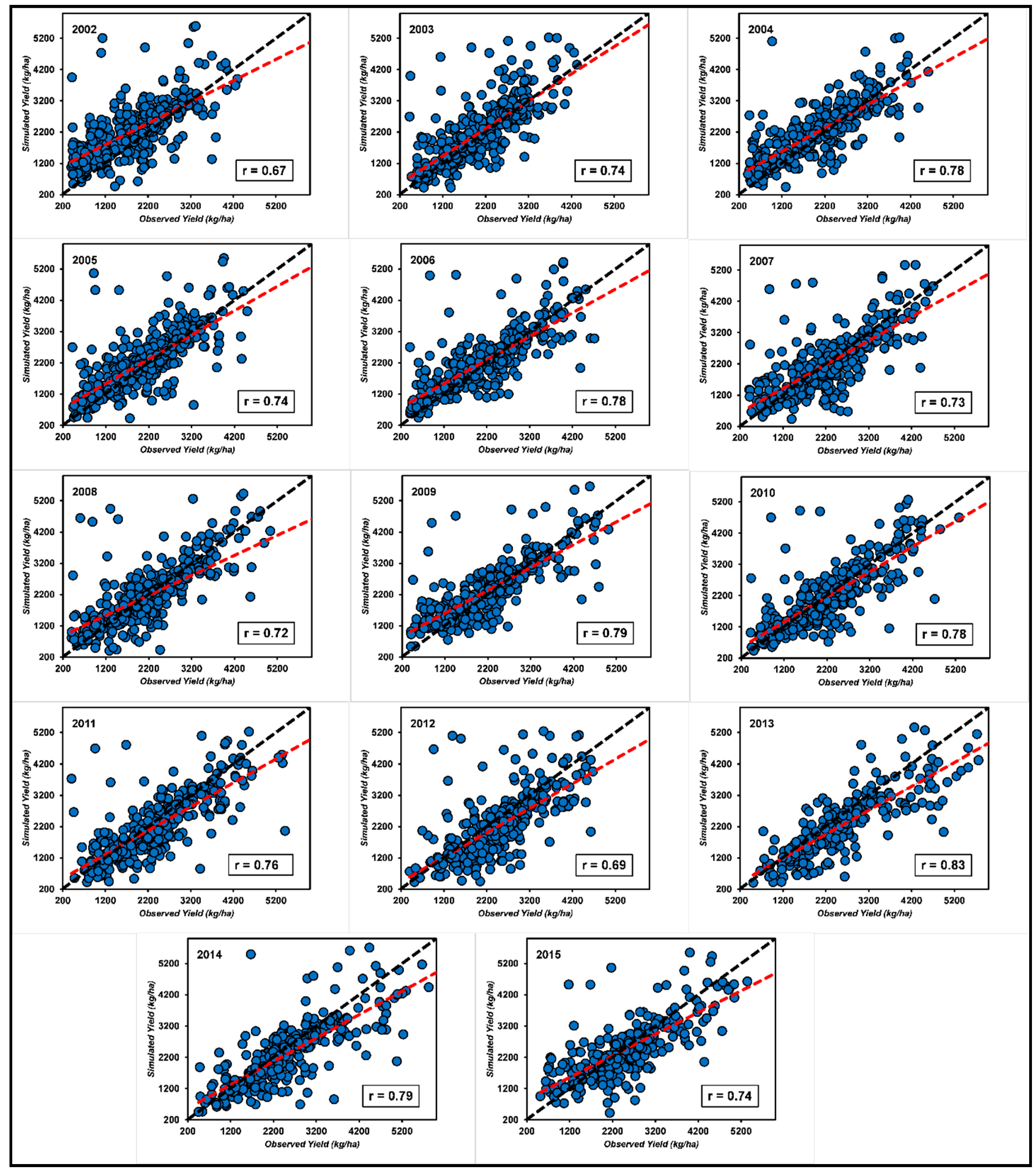
3.1. Model Calibration

After the calibration, the irrigation status was set to “irrigated” for around 90% of the pixels. Andhra Pradesh (Southern India), Jharkhand (Central East India), Karnataka (Southern India), Madhya Pradesh (Central India), Punjab (Northern India), Rajasthan (Northern India), Tamil Nadu (Southern India), and Telangana (Southern India) states were set to 2% to 22% rainfed after the calibration. Bihar (Eastern India) was set to 100% rainfed after calibration. The calibration showed that the best performing sowing dates were 160, 165, 175, and 195 Julian days. These dates were distributed over all the districts in the model simulation. Genetic co-efficient modified Swarna and Pusa-Suganth varieties dominantly worked for most of the states during the calibration. Table S4 shows the state-wise information of harmonized inputs after the calibration.

3.2. Long-Term Model Performance Assessment

Observed and simulated long-term average yields (2001 to 2015) were used to assess model performance across India. Figure 2 shows the pattern of the long-term average of district-wise observed yield (a) and the long-term average of simulated yield (b). The spatial pattern of the observed and simulated yields are highly similar. Overall, 76% of districts have an absolute yield error of less than 250 kg/ha, and 81% of districts have less than 350 kg/ha yield error. Figure 3 shows a good agreement between the long-term averages of state-wise observed and simulated yields.
We also compared state-wise observed and simulated yield by aggregating district-level yields. The simulation error of observed and simulated state aggregated yield is between –179 kg/ha to 110 kg/ha (Figure 3) except for Kerala (simulated yields are, on average, 615 kg/ha too low). The state-wise rRMSE and the Index of agreement (d) are shown in Table S5.
The model performance over the model calibration years (2001–2015) is exceptionally good, with 13 of 15 years achieving more than 0.7 correlation coefficient (r), and more than half of the years with above 0.75 correlation with observed yields. Only two years (2002 and 2012) had a moderate performance with r values of 0.67 and 0.69, respectively (Figure 4).

3.3. rRMSE of Yield Anomalies

Figure 5 shows the district wise spatial pattern of rRMSE between observed and simulated yield anomalies from 2001 to 2015. In comparison with all the states, Karnataka (Southern India), Telangana (Southern India), Andhra Pradesh (Southern India), West Bengal (Eastern India), Uttar Pradesh (Indo Gangetic—North), Haryana (Indo Gangetic Plains—North), Punjab (Northern India), and Uttarakhand (Himalayan region—North) have better rRMSE (0 to 25%) in almost all the districts except North Karnataka (Southern India), North Andhra Pradesh (Southern India), a few districts in Uttar Pradesh (Indo Gangetic Plains—North), and a few districts in Punjab (Northern India). At the same time, from low rice production states, Maharashtra and Gujarat, the Western Ghats districts of Maharashtra (Central India), and Western Gujarat (Western India) also produced a good rRMSE (0 to 25%). Many districts in the Indo Gangetic Plains, West Bengal, Karnataka, Telangana, Andhra Pradesh, and the Western Ghats of Maharashtra have <10% of rRMSE. A few districts in Orissa (Central East India) and Chhattisgarh (Central East India) produced moderate rRMSEs (10 to 25%). The states Madhya Pradesh (Central India), Bihar (Eastern India), Southern Chhattisgarh (Central East India), and the Vidharba regions of Maharashtra (Central India) produced poor rRMSE ( >35%). Overall, the model performance diverges spatially, as shown in Figure 5. Out of the 372 districts included in our analysis, rRMSE lower than 20%, 25%, 30% or 35% was achieved for 43% (160 districts), 56%, (205 districts), 66% (246 districts), and 73% (273 districts) of the districts, respectively. However, out of these 372 districts, the major rice-growing districts where there is >25% crop cultivation [4] in the district were separated, and 234 districts remained. Out of these 234 districts, rRMSE lower than 20% and 25% was achieved for 52% (122 districts) and 67% (157 districts) of the districts, respectively.

3.4. Index of Agreement (d) of Yield Anomalies

Figure S4 shows the spatial distribution of the model performance (the Index of agreement [d]) between the observed and simulated yield anomalies from 2001 to 2015. This Index of agreement (d) can perceive additive and proportional differences in the observed and simulated means and variances. The average agreement over India is 0.4, and values range from 0 to 0.87. Only 18% of districts have the Index of agreement (d) greater than 0.6. The states West Bengal (Eastern India) and Chhattisgarh (Eastern central India) produced the Index of agreement (d) of >0.5. The states Telangana (Southern India), Andhra Pradesh (Southern India), Karnataka (Southern India), Orissa (Eastern Central India), Tamil Nadu (Southern India), Uttarakhand (Himalayan Region), Punjab (Northern India), and Haryana (Northern India) produced moderate Index of agreement (d) (0.4 to 0.7) in most of the districts. Overall, out of 372 observed district yields, the model has produced >0.8, >0.7, and >0.6 the Index of agreement (d) for 5, 19, and 48 districts, respectively.

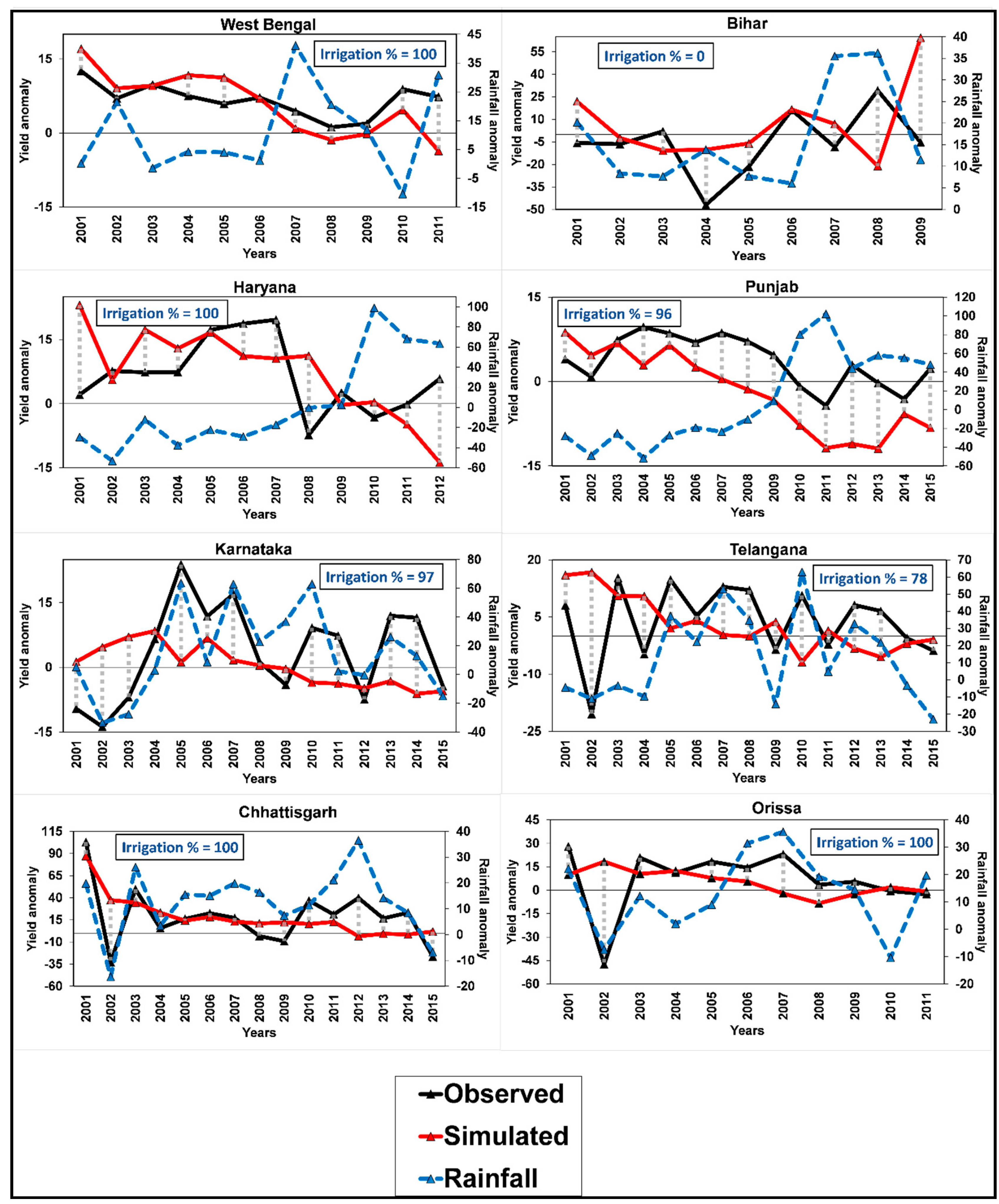
3.5. Effect of Rainfall on Yield Anomalies

The time series analysis between the simulated and observed rice yield anomalies from 2001 to 2015 are shown in Figure 6 for the various regions such as Eastern India, Indo Gangetic Plains, Eastern Central India, and Southern India. These are the major rice-growing regions in India (West Bengal and Bihar are from the Eastern India region, Haryana and Punjab are from Indo Gangetic Plains, Chhattisgarh and Orissa are from the East central region, and Karnataka and Telangana from the Southern region). The variability of observed yields is lower in irrigated rice areas, which is also replicated by the model (State-wise irrigation area percentage was mentioned in the plots). For example, in West Bengal, the model was able to match the observed rice yields for the period under assessment. Similarly, good model performance is observed in other states. However, there is a big difference between the simulated and observed rice yield anomalies for many states for the year 2002 (an extremely dry year). For example, there was a difference of 40% in Telangana and 15% in Karnataka. Interestingly, Bihar had a good model fit for 2002 but showed a big difference in 2009 (Figure 6). The in-season rainfall anomaly was plotted with yield anomalies to assess the impacts of precipitation on yields. Karnataka and Andhra Pradesh observed yield anomalies had a good fit with rainfall anomaly. In the states, Bihar, Chhattisgarh, and Orissa, both the observed and simulated yield anomalies had a good fit with in-seasonal rainfall anomaly. The irrigated states West Bengal, Haryana, Punjab, showed no effects of rainfall variation on yields. The time series plots for other states are shown in Figure S5.

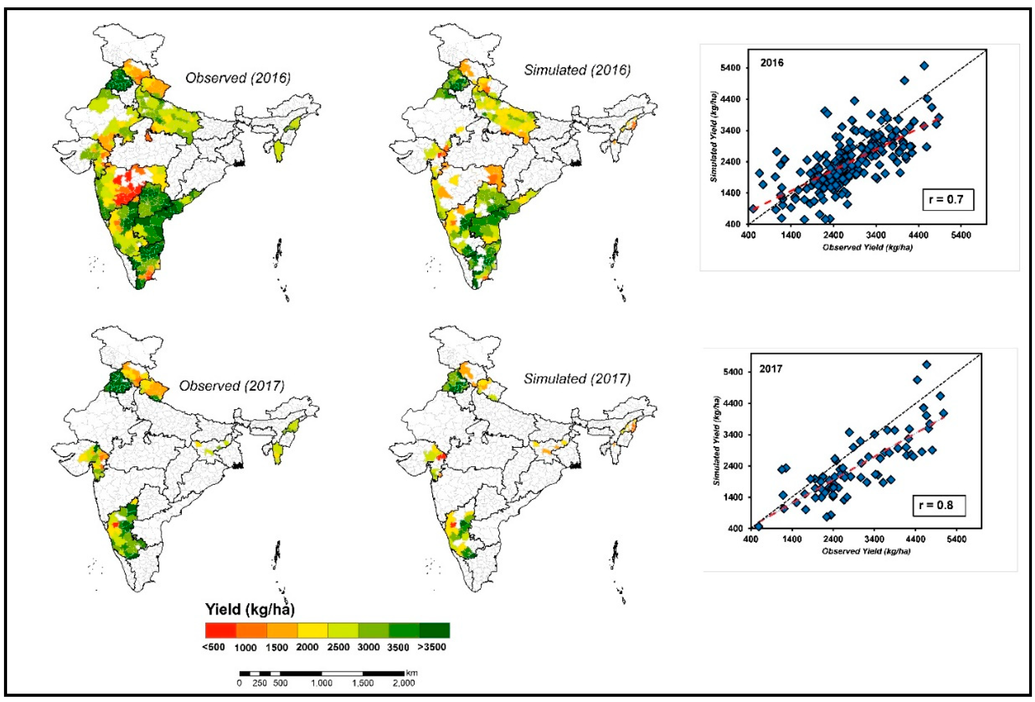
3.6. Model Validation

The model was calibrated with 2001 to 2015 observed yield anomalies. The calibrated model was then validated out-of-sample to test the model viability. We validated the model with the 2016 and 2017 Kharif season yield and yield anomalies. Figure S6a illustrates that all the states in Kharif 2016 analysis were simulated with at most ±20% error between observed and simulated yield anomaly except Gujarat (Central Western India) and Maharashtra (Central India). The model overpredicted the 2016 Kharif yield in the states Tamil Nadu and Karnataka but otherwise produced lower simulated yields in comparison with observed yields. Figure S6b shows that all the states in Kharif 2017 analysis have produced the ±20% error between observed and simulated anomalies except Himachal Pradesh (Himalayan Region), and the model underpredicted the yield loss for most the states in Kharif 2017.
In Maharashtra (Central India), the Kharif 2016 observed yield anomaly is registered 24.6% higher than the long-term average (2001–2015) observed yield anomaly. However, from the 2001 to 2015 yield series, the observed yield anomaly attained a maximum of 13% higher than the threshold yield, which is almost 100% lesser than Kharif 2016 observation in Maharashtra, and also the Kharif 2016 simulated yield is very close to the long-term observed average yield. These factors show that there is a chance of outlier observation for Maharashtra (Central India) in Kharif 2016. Similarly, the Gujarat (Central Western India) simulated yield is very close to the long-term observed yield, which also explains the chance of outlier in the Kharif 2016 observation. In Kharif 2017, all simulation errors (the difference between observed and simulated) were below 20% except Himachal Pradesh (22%). The state wise actual yields of observed and simulated was given in the Table S6 for the validation years.

3.7. Spatial Distribution Performance Evaluation

The comparison between district-level observed and simulated yields for the years 2016 and 2017 are shown in Figure 7. This spatial distribution of simulated yields shows that most of the districts have a good match with observed yields. The observed and simulated yields produced the correlation coefficients 0.68 (R2 = 0.46) and 0.79 (R2 = 0.63) for the years 2016 and 2017, respectively. In 2016, high rice productivity areas in the north (Punjab and Uttar Pradesh) and Southern states (Andhra Pradesh, Tamil Nadu, Telangana, and Karnataka) of India were simulated well. However, the model underestimated rice yield for the Vidharba regions of Maharashtra (Central India) and overestimated the Eastern parts of Tamil Nadu (Southern India). In 2017, even though there are very few observations, the model shows a good match with observed yields in most of the districts. Overall, 64% (34%) and 53% (43%) of districts produced the yields with a difference of –30% (–20%) to 30% (20%) from observed yields. The model underpredicted yields in many districts in both the years as many points were below the 1:1 line. However, the state-wise aggregation yield error for the year 2016 is from –18% to 29% except for Maharashtra (Central India), and for the year 2017 is from 17% to 32% except for Jharkhand (Eastern central). The ultimate outcome, 5 km spatial resolution yield, and yield anomaly maps are shown in Figure S7 and Figure S8, respectively, for the years 2016 and 2017.

4. Discussion

In this study, we calibrated and validated the DSSAT biophysical crop model to estimate rice yield anomalies for the Kharif season in India between 2001 and 2017, which are of potential interest for the PMFBY crop insurance scheme. Better-resolution real-time monitoring with publicly available data sets is a novel development for India. It could support the swift settling of crop insurance claims by in silico crop monitoring. Overall, model performance was satisfactory with spatial and temporal differences. These differences can be explained by differences in the intensity of rice production, gradients in growing seasons across India, and lacking consideration of extreme temperatures or other effects like pests and diseases in the crop model.

4.1. Data Quality

The quality of weather data plays a significant role in crop-growth modeling [47]. CHIRPS rainfall data has a good correlation with the station data in the majority of India. However, it contains a significant amount of uncertainties, especially in extreme cases [48]. Nevertheless, PMFBY requires the yield loss assessment to payout crop losses at 5 km, and CHIRPS is the available data at this resolution. In other studies, the combination of IMD and CHIRPS has produced a statistical rice yield model with a 2% yield error in India [47]. In terms of availability of observed yields for the purpose of calibration, India has sufficient observations except for East Central India (Chhatisgarh, Orrisa, Jharkhand, and Bihar) and Central India (Madhya Pradesh and Maharashtra). However, Central India is not a major rice-growing region except for the Western Ghats. Combining different data sources with idiosyncratic uncertainties is a potential source of errors in the model outputs. However, given the robust model performance in-sample and out-of-sample, we conclude that the publicly available data sources are of sufficient quality for crop modeling purposes on larger scales. Therefore, future modeling efforts at regional or national levels can be performed without the limitation of local data availability that hindered previous modeling efforts, as explained by [49]. In addition to uncertainty from the data sources, our filtering and standardization approaches may mask true signals and thus lead to model bias. We combined data from different sources and at various resolutions, requiring filtering of outliers and homogenization of input data before modeling [49,50]. In total, only 17% of the data were filtered and distributed over space and time, such that we assume that this step did not systematically influence results or conclusions.

4.2. Model Accuracy

The major rice-growing regions show better simulation results compared with other parts of India, most likely due to these regions having well-developed irrigation sources such as canals or bore wells, matching with our simulation settings of most pixels under irrigation [51]. Within these states, moderate model simulation skill is observed for a few districts as these parts have rainfed areas partially [45]. The poor rRMSE for Eastern districts in Tamil Nadu (Southern India) can be explained by the possibility of “late samba” [52] rice season (September–October) dominance; meanwhile, our model was calibrated using the sowing dates from the Julian day 160 onwards (June/July). “Late samba” is the rice season in Tamil Nadu (Southern India), where sowing starts in September–October and harvesting in December–January. Central India districts have less area under rice cultivation, which is also scattered over the states. Thus, our rice mask could miss actual rice pixels for aggregation in the simulated yields, which could be the reason for poor rRMSE between observed and simulated yield anomalies in these districts [30,53].
Moreover, PMFBY guidelines state that defining a crop as a major crop for deciding the Insurance Unit level, the sown area of that crop should be at least 25% of Gross Cropped Area in a District/Taluka or equivalent level [4]. In this case, rice is not a major crop in most of the districts from Central India. Thus, districts with higher rice densities produced better, more accuracy compared with other parts as these districts have more intense rice cultivation areas [30,53]. Thus, our model was able to simulate rice yields for the important rice areas correctly. The model underpredicted yields in many of the districts, highlighting that inputs may need to be updated with the latest farming practices, especially cultivars. The automated model calibration where sowing dates, cultivars, and irrigation were selected for each district did not result in model overfitting, indicating that all input choices are somewhat reasonable, as results after calibration mostly match with known agricultural practices and, most importantly, with the out-of-sample assessment which provides an indication for model quality.

4.3. Time Series Trend Analysis

The ability of the model to represent trends in rice yields was evident in most of the states. This indicates that the quality of input data and model was sufficient for rice modeling in India. Compared to previous studies that used process-based modeling for yield estimation in India [8,14], this study has provided 5km spatial resolution long-term spatially disaggregated yields at the national level. The time series trend analysis for both simulated and observed rice yields did not have much variance as the majority of rice is irrigated, with six of the major rice-producing states having over 75% rice under irrigation [54]. However, the time series trend analysis showed that the model overestimated the yield in 2002, which was an exceptional drought year [55]. This is explained by the fact that the model is not a coupled hydrological-crop-model and therefore assumes water is available for irrigation from various sources such as reservoirs, canal, river, etc., when needed, which was not the case in 2002. Possible overestimation for 2007, 2010, and 2011 can be explained by losses shortly before and during the harvest, which is not captured in the model. For example, Cardoen, D et al. (2015) pointed out that these harvest losses are significant factors affecting rice-farmers, especially when sudden extreme rainfall occurs during harvest [56]. However, in general, we conclude that the model is able to predict weather impacts under the rainfed conditions and under irrigated conditions, even though rainfall extremes hardly affect yields in irrigated areas except for extreme cases as in 2002.

4.4. Model Applicability for Crop Insurance

The yield simulation error of ±20% indicates that near-real-time crop monitoring is feasible and could be put into operational practice as Elabed et al. (2013) state that the maximum allowable probability of the yield prediction error for agricultural insurance applications should not exceed 20% [57]. In addition, this may prove useful for crop insurance applications within PMFBY, which limits differences in the estimation of yield for insurance purposes to 25% [4]. With the null model (long-term average of observed yields) comparison with simulated yields, we found no relationship (R2 < 0.0001) for all of the districts showing that the model is better than random prediction. Some studies have used DSSAT to estimate rice yields at the regional scale [42,58] with calibration based on field observations, but national-level yield estimation with DSSAT for India is limited so far. However, there are studies on rice yield estimation using GEPIC bio-physical crop model at the global and national scale. These studies reported that for the large countries, such as the USA, China, and India, the GEPIC model should be calibrated and validated on a smaller than national scale. Specifically for India, the GEPIC model underestimated rice in the southernmost part of India, whereas the other places gave a good correlation between the simulated and observed values [8]. Moreover, validation over these studies was carried out based on state-level aggregated yields, and simulations are at 50 km or 10 km spatial resolutions [8,14]. These resolutions are not sufficient to settle claims for widespread damage. The PMFBY scheme defines an insurance unit at to village or panchayat level. Our approach, conducted on 5 km resolution and evaluated on the district level, can bridge this gap. Simulated crop anomalies can be obtained shortly after harvest (at most two weeks, due to lag times in input data availability). Rapid payouts of indemnities could help farmers to recover from losses quickly and keep them in farming, which fosters national food security, enable farmers to invest in adaptation measures and could also slow rural-urban migration [59]. In addition, the transaction costs, usually involved with crop status or loss assessments (travel, field data collection, labor charges, processing charges), are reduced by our model-based approach. This can reduce insurance premiums and, thus, make insurances more affordable for Indian farmers.

5. Conclusions

This study presents ways to access and use available public datasets for reliable near-real-time rice crop simulations in India—a major rice producer—using a biophysical crop modeling approach. Calibrated simulations at 5 km resolution were able to attain an rRMSE of less than 20% between observed and simulated yield anomalies in almost half of all rice-growing districts. We conclude that it is possible to model rice yield at 5 km resolution reliably. Since the outputs are available soon after harvest, our study provides near real-time in-season crop monitoring for application in crop insurance decisions, particularly the Indian governmental PMFBY scheme for Kharif rice. Using such a model provides near real-time in-season crop monitoring for multiple decision applications but especially for immediate payouts for insurance. The late payment for an insurance payout has been a major problem in current crop insurance schemes in India, with its widespread impacts on farmers’ livelihoods and food security. We further conclude that it is possible to use open-source gridded crop model inputs for reliable rice crop modeling. This means that crop modeling can be successfully developed and applied with these data sources in many parts of the world with data paucity and yet may require modeling results for climate impact studies, food security assessments, yield gap studies, or understanding of drivers of yield. An update of inputs and simulations with the latest farming practices and crop mask as soon as these are available could further improve result accuracy. We would also highly appreciate an update of our results once an improved and more recent Kharif rice crop mask is available. Future work should focus on developing crop-model-based operational guidelines for insurance in India, multiple crop simulation, and also the capture of both seasons and not just the Kharif.

Supplementary Materials

The following are available online at https://www.mdpi.com/2073-4395/10/11/1674/s1, Figure S1: The number of observations available from DES district level yields between 2001 and 2016 for Kharif rice; Figure S2: The spatial distribution map for rice mask from very high-resolution MODIS multispectral rice classification, and derived 0.05° spatial resolution crop mask. a. Rice distribution under various irrigation types such as wetlands, deep water, upland, Irrigated, and rainfed. The crop names show the crop rotation (i.e., “Rice/Rice” means rice grows over the pixel both seasons (Kharif/Rabi)). b. Derived rice area distribution map in 5km resolution, based on the MODIS data in a map (a); Figure S3: Map of the fertilizer (N) application for Kharif rice in India; Figure S4: District-specific d values and histogram of the number of observations and the range of d. The histogram chart has d values as the X-axis and the number of districts as the Y-axis; Figure S5: Time series of observed and simulated yield anomalies and rainfall anomalies. Curves are observed yield anomalies (Observed, green), simulated yield anomalies (Simulated, magenta), and rainfall anomalies (Rainfall, blue). The left Y-axis represents the observed and simulated yield anomalies; the right Y-axis represents the rainfall anomaly. Years are on the X-axis. The red dotted lines show the error between observed and simulated yield anomalies; Figure S6: The grouped boxplots of observed and simulated yield anomalies for the years 2016 and 2017. The blue boxplots represent the observed yield anomalies; the red boxplots represent the simulated yield anomalies; The number of observations was given above the boxplot; the line in the boxplots are median; squared black dots are mean and red diamond dots are the outliers. Plot a consists of states from Southern India, plot b consists of states from Central India and Northern India, and plot c consists of states from Northern India and the Himalayan regions; Figure S7: The high-resolution spatial distribution map of actual yield for Kharif 2016 (left-hand side) and Kharif 2017 (right-hand side); Figure S8: The high-resolution spatial distribution map of yield loss for Kharif 2016 (left-hand side) and Kharif 2017 (right-hand side); Table S1: The states and their acronyms of the study area. The symbol * represents the selected states for this study, according to data availability (see below); Table S2: The varieties and calibrated genetic coefficients were used in this study; Table S3: The parameters used for analyzing the assessment of goodness index; Table S4: The state-wise information on inputs such as varieties used, sowing date, and irrigation status over the pixels within the state after the calibration; Table S5: State-wise average of RMSE and d which explains the goodness index of simulated yield loss with observed yield loss; Table S6: The state-wise observed and simulated yield information for the Kharif 2016 and 2017. The green shadowed data shows a <500 kg error. The unit of the data is kg/ha.

Author Contributions

Conceptualization, P.A., A.C., B.S., C.G.; methodology, P.A., B.S.; software, P.A., A.C.; validation, P.A., A.C., C.G.; formal analysis, P.A., A.C., B.S., C.G.; writing—original draft preparation, P.A., A.C.; writing—review and editing, A.C., B.S., C.G.; visualization, P.A.; supervision, C.G.; All authors have read and agreed to the published version of the manuscript.

Funding

The East Africa Peru India Climate Capacities (EPICC) project funded this research within the International Climate Initiative (IKI) funded by the German Federal Ministry for the Environment and Nature Conservation, and Nuclear Safety (BMU).

Acknowledgments

We are grateful to the Indian Meteorological Department (IMD), Directorate of Economics and Statistics (DES), International Soil Reference and Information Centre (ISRIC), Socioeconomic Data and Applications Center (SEDAC), and International Rice Research Institute (IRRI) for making their data available for this analysis. We would like to thank the East Africa Peru India Climate Capacities (EPICC) project for funding this research within the International Climate Initiative (IKI) funded by the German Federal Ministry for the Environment and Nature Conservation, and Nuclear Safety (BMU).

Conflicts of Interest

The authors declare no conflict of interest.

References

  1. Gulati, A.; Terway, P.; Hussain, S. Crop Insurance in India: Key Issues and Way Forward; Working Paper 352; Econstor: Kiel, Germany, 2018. [Google Scholar]
  2. Rai, R. Pradhan Mantri Fasal Bima Yojana: An Assessment of India’s Crop Insurance Scheme; Centre for Science and Environment: New Delhi, India, 2019; p. 16. [Google Scholar]
  3. GRiSP. A CGIAR Program on Rice-Based Production Systems; Global Rice Science Partnership (GRiSP): Cotonou, Benin, 2011. [Google Scholar]
  4. Pradhan Mantri Fasal Bima Yojana (PMFBY). Revised Guidelines; Ministry of Agriculture & Farmers Welfare, Government of India: New Delhi, India, 2017.
  5. Geethalakshmi, V.; Lakshmanan, A.; Rajalakshmi, D.; Jagannathan, R.; Sridhar, G.; Ramaraj, A.P.; Bhuvaneswari, K.; Gurusamy, L.; Anbhazhagan, R. Climate change impact assessment and adaptation strategies to sustain rice production in Cauvery basin of Tamil Nadu. Curr. Sci. 2011, 101, 6. [Google Scholar]
  6. Lal, M.; Singh, K.K.; Rathore, L.S.; Srinivasan, G.; Saseendran, S.A. Vulnerability of rice and wheat yields in NW India to future changes in climate. Agric. For. Meteorol. 1998, 89, 101–114. [Google Scholar] [CrossRef]
  7. Mishra, A.; Singh, R.; Raghuwanshi, N.S.; Chatterjee, C.; Froebrich, J. Spatial variability of climate change impacts on yield of rice and wheat in the Indian Ganga Basin. Sci. Total Environ. 2013, 468–469, S132–S138. [Google Scholar] [CrossRef]
  8. Priya, S.; Shibasaki, R. National spatial crop yield simulation using GIS-based crop production model. Ecol. Model. 2001, 136, 113–129. [Google Scholar] [CrossRef]
  9. Sudharsan, D.; Adinarayana, J.; Reddy, D.R.; Sreenivas, G.; Ninomiya, S.; Hirafuji, M.; Kiura, T.; Tanaka, K.; Desai, U.B.; Merchant, S.N. Evaluation of weather-based rice yield models in India. Int. J. Biometeorol. 2013, 57, 107–123. [Google Scholar] [CrossRef]
  10. Asseng, S.; Martre, P.; Maiorano, A.; Rötter, R.P.; O’Leary, G.J.; Fitzgerald, G.J.; Girousse, C.; Motzo, R.; Giunta, F.; Babar, M.A.; et al. Climate change impact and adaptation for wheat protein. Glob. Chang. Biol. 2019, 25, 155–173. [Google Scholar] [CrossRef] [Green Version]
  11. Basso, B.; Ritchie, J.T.; Pierce, F.J.; Braga, R.P.; Jones, J.W. Spatial validation of crop models for precision agriculture. Agric. Syst. 2001, 68, 97–112. [Google Scholar] [CrossRef]
  12. Folberth, C.; Elliott, J.; Müller, C.; Balkovič, J.; Chryssanthacopoulos, J.; Izaurralde, R.C.; Jones, C.D.; Khabarov, N.; Liu, W.; Reddy, A.; et al. Parameterization-induced uncertainties and impacts of crop management harmonization in a global gridded crop model ensemble. PLoS ONE 2019, 14, e0221862. [Google Scholar] [CrossRef] [Green Version]
  13. Irmak, A.; Jones, J.W.; Batchelor, W.D.; Paz, J.O. Estimating Spatially Variable Soil Properties for Application of Crop Models in Precision Farming. Trans. ASAE 2001, 44. [Google Scholar] [CrossRef]
  14. Liu, J.; Williams, J.R.; Zehnder, A.J.B.; Yang, H. GEPIC – modelling wheat yield and crop water productivity with high resolution on a global scale. Agric. Syst. 2007, 94, 478–493. [Google Scholar] [CrossRef]
  15. Rosenzweig, C.; Elliott, J.; Deryng, D.; Ruane, A.C.; Müller, C.; Arneth, A.; Boote, K.J.; Folberth, C.; Glotter, M.; Khabarov, N. Assessing agricultural risks of climate change in the 21st century in a global gridded crop model intercomparison. Proc. Natl. Acad. Sci. USA 2014, 111, 3268–3273. [Google Scholar] [CrossRef] [Green Version]
  16. Awad, M. Toward Precision in Crop Yield Estimation Using Remote Sensing and Optimization Techniques. Agriculture 2019, 9, 54. [Google Scholar] [CrossRef] [Green Version]
  17. Shiu, Y.-S.; Chuang, Y.-C. Yield Estimation of Paddy Rice Based on Satellite Imagery: Comparison of Global and Local Regression Models. Remote Sens. 2019, 11, 111. [Google Scholar] [CrossRef] [Green Version]
  18. Jin, X.; Kumar, L.; Li, Z.; Feng, H.; Xu, X.; Yang, G.; Wang, J. A review of data assimilation of remote sensing and crop models. Eur. J. Agron. 2018, 92, 141–152. [Google Scholar] [CrossRef]
  19. Son, N.T.; Chen, C.F.; Chen, C.R.; Chang, L.Y.; Chiang, S.H. Rice Yield Estimation Through Assimilating Satellite Data Into A Crop Simumlation Model. Int. Arch. Photogramm. Remote Sens. Spat. Inf. Sci. 2016, 8, 993–996. [Google Scholar] [CrossRef]
  20. Wang, D.; Wang, J.; Liang, S. Retrieving crop leaf area index by assimilation of MODIS data into a crop growth model. Sci. China Earth Sci. 2010, 53, 721–730. [Google Scholar] [CrossRef]
  21. Kamilaris, A.; Kartakoullis, A.; Prenafeta-Boldú, F.X. A review on the practice of big data analysis in agriculture. Comput. Electron. Agric. 2017, 143, 23–37. [Google Scholar] [CrossRef]
  22. Aggarwal, P.K.; Shirsath, P.; Arumugam, P.; Goroshi, S.; Nagpal, M.; Vyas, S. Monitoring weather deviations and crop conditions for agriculture insurance in India. Csalp South. Asia Q. Newsl. 2018, 1, 11. [Google Scholar]
  23. Hoogenboom, G.; Porter, C.H.; Shelia, V.; Boote, K.J.; Singh, U.; White, J.W.; Hunt, L.A.; Ogoshi, R.; Lizaso, J.I.; Koo, J. Decision Support System for Agrotechnology Transfer (DSSAT) Version 4.7; DSSAT Foundation: Gainesville, FL, USA, 2017. [Google Scholar]
  24. Jones, J.W.; Hoogenboom, G.; Porter, C.H.; Boote, K.J.; Batchelor, W.D.; Hunt, L.A.; Wilkens, P.W.; Singh, U.; Gijsman, A.J.; Ritchie, J.T. The DSSAT cropping system model. Eur. J. Agron. 2003, 18, 235–265. [Google Scholar] [CrossRef]
  25. R Core Team. R: A Language and Environment for Statistical Computing; R Foundation for Statistical Computing: Vienna, Austria, 2018. [Google Scholar]
  26. ESRI. ArcMap 10.7.1; ESRI Inc.: Redlands, CA, USA, 2018. [Google Scholar]
  27. DES. Directorate of Economics and Statistics, Ministry of Agriculture and Farmers Welfare, Government of India. 2015. Available online: https://aps.dac.gov.in/APY/Index.htm (accessed on 7 October 2019).
  28. Sudduth, K.A.; Drummond, S.T. Yield Editor: Software for Removing Errors from Crop Yield Maps. Agron. J. 2007, 99, 1471–1482. [Google Scholar] [CrossRef]
  29. Vega, A.; Córdoba, M.; Castro-Franco, M.; Balzarini, M. Protocol for automating error removal from yield maps. Precis. Agric. 2019, 20, 1030–1044. [Google Scholar] [CrossRef]
  30. Gumma, M.K. Mapping rice areas of South Asia using MODIS multitemporal data. J. Appl. Remote Sens. 2011, 5, 053547. [Google Scholar] [CrossRef] [Green Version]
  31. The World Bank Group. Agricultural Land (% of Land Area); Food and Agriculture Organization: Rome, Italy, 2019. [Google Scholar]
  32. Funk, C.; Peterson, P.; Landsfeld, M.; Pedreros, D.; Verdin, J.; Shukla, S.; Husak, G.; Rowland, J.; Harrison, L.; Hoell, A. The climate hazards infrared precipitation with stations—A new environmental record for monitoring extremes. Sci. Data 2015, 2, 150066. [Google Scholar] [CrossRef] [Green Version]
  33. Srivastava, A.K.; Rajeevan, M.; Kshirsagar, S.R. Development of a high resolution daily gridded temperature data set (1969–2005) for the Indian region. Atmos. Sci. Lett. 2009. [Google Scholar] [CrossRef]
  34. Mahmood, R.; Hubbard, K.G. Effect of time of temperature observation and estimation of daily solar radiation for the Northern Great Plains, USA. Agron. J. 2002, 94, 723–733. [Google Scholar] [CrossRef] [Green Version]
  35. Hengl, T.; de Jesus, J.M.; Heuvelink, G.B.; Gonzalez, M.R.; Kilibarda, M.; Blagotić, A.; Shangguan, W.; Wright, M.N.; Geng, X.; Bauer-Marschallinger, B. SoilGrids250m: Global gridded soil information based on machine learning. PLoS ONE 2017, 12, e0169748. [Google Scholar] [CrossRef] [Green Version]
  36. Hengl, T.; de Jesus, J.M.; MacMillan, R.A.; Batjes, N.H.; Heuvelink, G.B.; Ribeiro, E.; Samuel-Rosa, A.; Kempen, B.; Leenaars, J.G.; Walsh, M.G. SoilGrids1km—Global soil information based on automated mapping. PLoS ONE 2014, 9, e105992. [Google Scholar] [CrossRef] [Green Version]
  37. International Research Institute for Climate and Society (IRI); Michigan State University (MSU); HarvestChoice/International Food Policy Research Institute (IFPRI). Global High.-Resolution Soil Profile Database for Crop Modeling Applications; International Research Institute for Climate and Society (IRI): New York, NY, USA; Michigan State University: East Lansing, MI, USA; International Food Policy Research Institute (IFPRI): Washington, DC, USA, 2015. [Google Scholar]
  38. Shangguan, W.; Hengl, T.; de Jesus, J.M.; Yuan, H.; Dai, Y. Mapping the global depth to bedrock for land surface modeling. J. Adv. Model. Earth Syst. 2017, 9, 65–88. [Google Scholar] [CrossRef]
  39. Han, E.; Ines, A.; Koo, J. Global High-Resolution Soil Profile Database for Crop. Modeling Applications; Working Paper; HarvestChoice/International Food Policy Research Institute: Washington, DC, USA, 2015. [Google Scholar]
  40. Potter, P.; Ramankutty, N.; Bennett, E.M.; Donner, S.D. Global Fertilizer and Manure, Version 1: Nitrogen Fertilizer Application; NASA Socioeconomic Data and Applications Center (SEDAC): Palisades, NY, USA, 2011. [Google Scholar]
  41. Lu, G.Y.; Wong, D.W. An adaptive inverse-distance weighting spatial interpolation technique. Comput. Geosci. 2008, 34, 1044–1055. [Google Scholar] [CrossRef]
  42. Jain, S.; Sastri, A.; Manikandan, N.; Chaudhary, J.L.; Kumar, B. Assessment of yield and yield attributes gap under irrigated and rainfed condition in rice crop for different agroclimatic zones of Chhattisgarh using DSSAT Simulation model. IJCS 2018, 6, 23–28. [Google Scholar]
  43. Satapathy, S.S.; Swain, D.K.; Herath, S. Field experiments and simulation to evaluate rice cultivar adaptation to elevated carbon dioxide and temperature in sub-tropical India. Eur. J. Agron. 2014, 54, 21–33. [Google Scholar] [CrossRef]
  44. Singh, K.K.; Baxla, A.K.; Chattopadhyay, N.; Balasubramanian, R.; Singh, P.K.; Rana, M.; Gohain, G.B.; Vishnoi, L.; Singh, P. Crop Yield forecasting under FASAL. In Forecasting Agricultural Output Using SPACE Agrometeorology and Land Based Observations; Indian Meteorological Department: Pune, India, 2017; p. 162. [Google Scholar]
  45. Lu, J.; Carbone, G.J.; Gao, P. Detrending crop yield data for spatial visualization of drought impacts in the United States, 1895–2014. Agric. For. Meteorol. 2017, 237–238, 196–208. [Google Scholar] [CrossRef]
  46. Ye, T.; Nie, J.; Wang, J.; Shi, P.; Wang, Z. Performance of detrending models of crop yield risk assessment: Evaluation on real and hypothetical yield data. Stoch. Environ. Res. Risk Assess. 2015, 29, 109–117. [Google Scholar] [CrossRef]
  47. Parkes, B.; Higginbottom, T.P.; Hufkens, K.; Ceballos, F.; Kramer, B.; Foster, T. Weather dataset choice introduces uncertainty to estimates of crop yield responses to climate variability and change. Environ. Res. Lett. 2019, 14, 124089. [Google Scholar] [CrossRef]
  48. Gupta, V.; Jain, M.K.; Singh, P.K.; Singh, V. An assessment of global satellite-based precipitation datasets in capturing precipitation extremes: A comparison with observed precipitation dataset in India. Int. J. Climatol. 2019. [Google Scholar] [CrossRef]
  49. Grassini, P.; van Bussel, L.G.J.; Van Wart, J.; Wolf, J.; Claessens, L.; Yang, H.; Boogaard, H.; de Groot, H.; van Ittersum, M.K.; Cassman, K.G. How good is good enough? Data requirements for reliable crop yield simulations and yield-gap analysis. Field Crop. Res. 2015, 177, 49–63. [Google Scholar] [CrossRef] [Green Version]
  50. Heuvelink, G.B. Error Propagation in Environmental Modelling with GIS; CRC Press: Boca Raton, FL, USA, 1998; ISBN 0-7484-0744-8. [Google Scholar]
  51. Roy, A.D.; Shah, T. Socio-ecology of groundwater irrigation in India. In Intensive Use of Groundwater: Challenges and Opportunities; Swets & Zeitlinger B.V.: Lisse, The Netherlands, 2002; pp. 307–335. [Google Scholar]
  52. TNAU. Tamil Nadu Cropping Season. In Expert System for Paddy; Tamil Nadu Agricultural University: Coimbatore, India, 2009. [Google Scholar]
  53. Xiao, X.; Boles, S.; Frolking, S.; Li, C.; Babu, J.Y.; Salas, W.; Moore, B., III. Mapping paddy rice agriculture in South and Southeast Asia using multi-temporal MODIS images. Remote Sens. Environ. 2006, 100, 95–113. [Google Scholar] [CrossRef]
  54. Handral, A.R.; Singh, A.; Singh, D.R.; Suresh, A.; Jha, G.K. Scenario of changing dynamics in production and productivity of major cereals in India. Indian J. Agric. Sci. 2017, 87, 1371–1376. [Google Scholar]
  55. Naresh Kumar, M.; Murthy, C.S.; Sesha Sai, M.V.R.; Roy, P.S. Spatiotemporal analysis of meteorological drought variability in the Indian region using standardized precipitation index. Meteorol. Appl. 2012, 19, 256–264. [Google Scholar] [CrossRef] [Green Version]
  56. Cardoen, D.; Joshi, P.; Diels, L.; Sarma, P.M.; Pant, D. Agriculture biomass in India: Part 2. Post-harvest losses, cost and environmental impacts. Resour. Conserv. Recycl. 2015, 101, 143–153. [Google Scholar] [CrossRef]
  57. Elabed, G.; Bellemare, M.F.; Carter, M.R.; Guirkinger, C. Managing basis risk with multiscale index insurance. Agric. Econ. 2013, 44, 419–431. [Google Scholar] [CrossRef]
  58. Kumar, A.; Nath, S.; Balpande, R.; Kumar, P.; Mishra, A.; Kumar, V. Decision support system for agro technology (DSSAT) modeling for estimation of rice production and validation. J. Pharmacogn. Phytochem. 2019, 8, 3883–3886. [Google Scholar]
  59. Chandrasekhar, S.; Sahoo, S. Short-Term Migration in Rural India: The Impact of Nature and Extent of Participation in Agriculture; Indira Gandhi Institute of Development Research: Mumbai, India, 2018. [Google Scholar]
Figure 1. The workflow of the study (a) and state boundaries in India (b) with a sample of grid cells (diameter of the circle is approximately 100 km2). The state acronyms are explained in Table S1.
Agronomy 10 01674 g001
Figure 2. The spatial distribution for district-wise observed and simulated long-term average yield (2001–2015). Figure (a) represents the observed, and Figure (b) represents the simulated yields.
Agronomy 10 01674 g002
Figure 3. Comparison of state-wise average observed and simulated yields. The figure was divided into geographical zones in India, such as Southern India (a), Eastern India (b), Central India (c), Indo Gangetic Plains and Western India (d), and Western Himalayan Region (e). Blue bars show observed yields, while grey bars show the simulated yields.
Agronomy 10 01674 g003
Figure 4. Comparison between district-level observed and simulated yield for the model calibration years (2001 to 2015). The black line describes a 1:1 ratio, and the red line explains the regression fit between observed and simulated yields.
Agronomy 10 01674 g004
Figure 5. District-wise relative Root Mean Square Error (rRMSE) as a map and as a histogram. The histogram shows rRMSE values on the X-axis and the number of districts on the Y-axis.
Agronomy 10 01674 g005
Figure 6. Time series of observed and simulated yield anomalies and rainfall anomalies. Curves are observed yield anomalies (Observed, black), simulated yield anomalies (Simulated, red), and rainfall anomalies (Rainfall, blue). The left Y-axis represents the observed and simulated yield anomalies; the right y-axis represents the rainfall anomaly. Years are on the X-axis. The grey dotted lines show the error between observed and simulated yield anomalies.
Agronomy 10 01674 g006
Figure 7. The spatial distribution comparison between aggregated district-level simulated yield and district-level observed yields for the years 2016 and 2017 and the scatterplot between observed and simulated yields for the years 2016 and 2017. There were fewer districts in simulated yields compared to observed yields due to the restriction of the crop mask.
Agronomy 10 01674 g007
Table 1. Types and description of gridded inputs used for rice simulation with the Decision Support System for Agrotechnology Transfer (DSSAT) in India.
Input CategoryDetailed Inputs
Weather (Daily)
  • Rainfall
  • Maximum temperature
  • Minimum temperature
  • Solar radiation
  • Average annual temperature
  • Temperature amplitude
Soil
  • Upper and lower horizon depths (cm),
  • Percentage of sand, silt, clay content
  • 1/3 bulk density, organic carbon
  • pH in water,
  • Aluminum saturation
  • Root abundance
Farmer’s practices
  • Planting date
  • Soil condition measurement date before planting
  • Planting density
  • Row spacing,
  • Planting depth
  • Crop variety
  • Irrigation practices and dates
  • Fertilizer amounts and dates
Publisher’s Note: MDPI stays neutral with regard to jurisdictional claims in published maps and institutional affiliations.

