Article

New Approach to the Assessment of Insecticide Losses from Paddy Fields Based on Frequent Sampling Post Application

College of Hydraulic Science and Engineering, Yangzhou University, Yangzhou 225009, China
*
Author to whom correspondence should be addressed.
Agronomy 2020, 10(10), 1615; https://doi.org/10.3390/agronomy10101615
Submission received: 16 September 2020 / Revised: 17 October 2020 / Accepted: 19 October 2020 / Published: 21 October 2020
(This article belongs to the Section Agricultural Biosystem and Biological Engineering)

Abstract

:
High concentration of insecticides may appear in waters surrounding paddy fields shortly after application. Capturing the dynamic feature of this insecticide pulse may help control insecticide load to receiving waters. Based on continuous monitoring of the drainage process and two monitoring campaigns of three insecticides—chlorpyrifos, abamectin and thiamethoxam—in a paddy, this study examined the pattern of insecticide concentrations at different locations of paddy waters during the period of insecticide application accompanied with pest-control irrigation, and analyzed the factors affecting the environmental behavior of these insecticides. The results showed that the pulse-type drainage exhibited the following features: short duration (normally less than 1 d), large flow rate (as large as 4 L s−1), frequent occurrence (20 times during a 40-d period) and long time interval (as long as 5 d). Concentrations of the insecticides with higher Henry’s constant and vapor pressure peaked quickly (within several hours) post application in the field ditch; more than half of chlorpyrifos and abamectin loads were detected within merely 1 h after application. The high insecticide concentrations in the ditch were partly attributed to the primary and secondary drift. Moreover, a new kinetic model was proposed to describe the behavior of chlorpyrifos at the field edge. It is recommended that controlled drainage be implemented for at least 1 d post application to prevent the loss of insecticides. Findings from this study may provide new insights into insecticide behavior in the paddy environment for preventing adverse environmental impacts.

Graphical Abstract

1. Introduction

Outbreaks of insects has become a major threat to rice production in southeastern Asia due to the enhancement of monsoon and the climate change effects. Insecticide application has been widely used to suppress periodic occurrence of variable pests in paddy fields in southeastern China, which is a major rice production area. To ensure a better killing effect, simultaneous irrigation is applied during the insecticide spray application; a surface ponding of 3–5 cm water layer in paddy fields may facilitate a fumigation condition and prevent insects from escaping. Such practice, however, creates a high potential of insecticide losses through drainage. Insecticides of high concentration in drainage water may pose potential risks to the aquatic system [1] and human health [2], and onsite monitoring of the insecticide losses is an important approach to assess the risk.
Insecticide loss in agricultural landscapes in humid eastern China is heavily affected by the prevalent rice cropping systems [3]. Water bodies accommodating aquatic communities surrounding paddy fields are exposed to high ecological risks [4,5]. In contrast to herbicides and fungicides, insecticides are designed to kill target pests before being quickly degraded and do not need to persist in natural environments for a long time [6]. Despite of this fact, even very short pulses (the rapid increase and decrease process of insecticide concentrations that could last from a few minutes to several hours) of insecticides can still pose high risks to aquatic organisms [7,8,9].
Several studies have paid attention to the pulse feature of pesticide behavior in the water environment. Atrazine concentrations at the tile drainage outlet of a corn farm increased to 34.5 μg L−1 during a storm event occurring 6 d after atrazine application and thereafter decreased to approximately 1 μg L−1 within 1 d, which was attributed to the preferential flow in soil [10]. The fenitrothion and dimethoate concentrations of fish pond water near paddy fields peaked on the day of application and decreased by approximately 90% within 1 d [11]. Pretilachlor concentration of paddy drainage water decreased by 90% within 4 d post application [12]. Sangchan et al. [13] applied high-frequency monitoring with sampling intervals of 1 h and found that the duration of pesticide pulse export was less than several hours during runoff peaks. Some other studies [14,15,16,17,18] observed that pesticide concentrations of paddy surface water peaked at the first sampling moment (2 h to 2 d after application).
Conventionally, the pesticide degradation processes in field surface water and drainage water are infrequently monitored because of the high monitoring expenses and are described by the first-order kinetic model [15,17,19]. To date, a minority of studies have focused on the variation of pesticide concentrations within sub-hourly time intervals at watershed or larger scales [13,20,21]. Field-scale insecticide behavior at short temporal scales in water environments remains unexplored. The presently available kinetic models reviewed by [22] perform well in describing the degradation process after pesticide concentration peaks, but the period of rapid increase before the peak post application has not received close attention. To the best of our knowledge, existing studies are limited in monitoring and modeling the whole process of insecticide loss from paddies via surface runoff.
Assuming that the pulse-type insecticide export with drainage process exists in paddy fields, this study presents a monitoring study of frequent sampling in paddy waters at time intervals of as short as 1 h after insecticide applications; three commonly used insecticide chlorpyrifos (CPF), abamectin (ABM) and thiamethoxam (THM) were sampled in different waters of a typical paddy environment in southeastern China. The specific objectives of this study were to
(1)
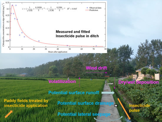
capture the dynamic features of drainage and insecticide pulses in the field drainage ditch of paddy fields shortly after application,
(2)
identify the key factors that affect insecticide behavior and establish a kinetic model that can better describe the edge-of-field insecticide concentration variations, and
(3)
analyze the influence of sampling strategies on monitoring results and propose drainage control strategies after insecticide application in rice growing areas.

2. Materials and Methods

2.1. Study Area

The experiment was conducted in the Yanyun Irrigation District (119°30′ E, 32°33′ N) located to the east of the Grand Canal in southeastern China. The area lies in the subtropical monsoon climate zone where rice–wheat rotation is the most prevalent cropping pattern; rice is generally grown in the rainy season between June and October, but supplemental irrigation still is required to meet the high water consumption of rice. Paddy fields are generally divided into 100 × 100 m2 plots bounded with drainage ditches of 60 cm deep. Figure 1 shows the experimental paddy fields of this study as delineated with the orange line. A v-notch weir was installed at the field ditch outlet as marked with the gray triangle. The water level of the ditch was measured with a water level data logger (HOBO U20-001-04 Onset) installed near the weir at the bottom of the ditch; drainage flow rate was calculated from the recorded water level data at 15-min intervals during the first sampling event and at 5-min intervals during the second sampling event. An empirical equation was applied to calculate the flow rate of the field ditch [23].
Q = 8 15 μ tan θ 2 2 g h 5 2
where Q is the calculated flow rate of the field ditch passing through the weir (L s−1); μ is the flow coefficient. The ditch flow rate was measured manually for 13 times to calibrate the equation, and μ was determined to be 0.74 when the deviation of calculated and measured flow rate values was minimum; θ is the angle of the weir notch (°), which was measured to be 45; g is the acceleration of gravity (9.808 m s−2); h is the water head above the weir notch (m).
Weather data, including rainfall, wind speed and direction, air temperature, radiation and humidity were recorded at time intervals of 15 min by a weather station (CR1000, Campbell Scientific, Logan, UT, USA) near the study site (Figure 1). More details of the study area are available in [24,25].

2.2. Insecticide Application and Sampling Procedure

In 2018, during the booting and internode elongation stages of rice, the paddy were attacked by Cnaphalocrocis medinalis (Guenée) outbreaks. During the whole rice growing period (15 June to 29 November, 2018), two insecticides were applied for the control of Cnaphalocrocis medinalis and other potential insects. The insecticides chlorpyrifos (CPF, produced by Dow Chemical Company, 40% active substance, emulsifiable concentrate, EC) and abamectin (ABM, produced by Syngenta, 1.8% active substance, EC), together with two fungicides were applied on 11 August 2018. The insecticides thiamethoxam (THM, produced by Syngenta, 25% active substance, water dispersible granule), ABM (1.8% active substance, EC) and a mixture of emamectin benzoate (2.5% active substance, wettable powder, WP) and Bacillus thuringiensis (8000 IU mg−1, WP), together with two other fungicides were applied on 2 September 2018. The applied amounts of CPF, ABM (during the first application event) and THM were 384, 10.8 and 30 g a.i. ha−1 (gram active ingredient per hectare), respectively. Both of the two applications were conducted with the same sprayers (volume: 18 L, maximum pressure: 0.40 mPa). Table 1 lists the physico-chemical properties of the three concerned insecticides. On 12 June, 2018, water samples were collected at the outlet of the field ditch, paddy surface water and the sampling well to assess the residues of CPF, ABM and THM before the two applications.
During the first insecticide application event, spraying was conducted between 6:00 a.m. and 7:33 a.m. from west to east sides of the field, while irrigation was applied between 5:48 a.m. and 7:00 a.m. to enhance the insect killing effect. Drainage outflow was observed at the field ditch outlet between 6:11 a.m. and 12:45 p.m. The first batch of water samples were taken at 7:45 a.m. at the midpoint and outlet of the field ditch, as well as the paddy surface and sampling well (as shown in Figure 1). During the second application event, insecticides were applied to paddy fields between 6:33 a.m. and 10:06 a.m., and irrigation was applied between 6:26 a.m. and 8:19 a.m. Drainage outflow occurred between 7:18 a.m. and 9:53 a.m. During the two sampling events, all the drainage outlets of the paddy plots were closed.
When drainage outflow occurred at the ditch outlet, water samples were collected downstream near the weir; otherwise, they were collected upstream near the weir. In the first sampling event, surface grab water samples were collected at 0, 1, 2, 3, 4, 5, 6, 8, 10, 12, 24, 36, 48 and 72 h after insecticide application. The volume of each water sample was approximately 500 mL. Water samples from the sampling well were taken at 0, 2, 4, 6, 8, 10, 12, 24, 36, 48 and 72 h after application. At 72 h after insecticide application, ponding water at the paddy soil surface diminished to small puddles where water samples were taken. In the second sampling event, water samples were taken only at the two sampling points in the field ditch. Water samples were taken at 9:17 a.m. (−1 h) and 10:27 a.m. (0 h), and they were then taken at 1.5, 2, 3, 4, 5, 6, 8, 10 and 12 h after application at both points. All the samples were immediately stored in the freezer at −18 °C in the nearby experimental station. Upon completion of sampling events, all samples were shipped in ice boxes to a certified chemistry laboratory for chemical analysis. A total of 92 water samples were extracted for analysis (53 for CPF, 17 for ABM and 22 for THM).
CPF and THM were measured by a GC–MS system (7890B gas chromatograph equipped with 5977B single quadrupole mass spectrometry detector, Agilent Technologies, Santa Clara, CA, USA) with an HP-5MS column. ABM was measured by an LC–MS system (TSQ Quantum Access MAX triple-quadrupole mass spectrometer, Thermo Fisher Scientific, Waltham, MA, USA) with an SB-C18 column. A 100-mL volume of each collected water sample (500 mL) was extracted for three times with methylene dichloride (20 mL). The extracts were then combined and mixed for 3 min before anhydrous sodium sulfate (10 g) was added in. The supernatant was collected and dried with a termovap nitrogen sample concentrator (Anpel Laboratory Technologies, Shanghai, China) and was then adjusted to volumes of 4 mL (for CPF) and 2 mL (for ABM and THM) with acetone for GC–MS analysis. The pre-treatment process of ABM was almost the same, except that the supernatant was finally adjusted to a 2-mL volume with methyl alcohol for LC–MS analysis. For each water sample, two subsamples of 100 mL were measured. Two duplicate measurements of each sample were compared to ensure the measurement accuracy. The detection limits of CPF, ABM and THM were 0.000504, 0.0001 and 0.001 mg L−1, respectively.

2.3. Estimation of Insecticide Load and Concentration Kinetics

Edge-of-field insecticide loads can be calculated as the product of field ditch discharge and insecticide concentration at the ditch outlet measured at the same time. Since drainage discharge was measured at shorter time intervals than insecticide concentration, linear interpolations were adopted to calculate insecticide concentrations between two time intervals for load estimation.
c i = c II c I t II t I ( t i t I ) + c I
where ci (mg L−1) is the interpolated insecticide concentration at the moment of ti; cI and cII (mg L−1) are the measured insecticide concentrations at the moments tI and tII, respectively [27]. For instance, in order to match water samples taken at 1-h intervals with the drainage discharge data recorded at 15-min intervals, three concentration data points need to be interpolated for insecticide load estimation at 15-min intervals. The insecticide load was calculated by [21].
L i j = ( c i Q i + c j Q j ) ( t j t i ) / 2
where Li-j (mg) is the calculated insecticide export load from the moments ti to tj; ci and cj (mg L−1) are measured or interpolated insecticide concentration at the moments ti and tj; Qi and Qj are measured drainage flow rate at the ditch outlet (L s−1).
Since the area of the paddy field is 1 ha, the value of calculated total insecticide load in the study area is equal to the areal loading rate.
The Curve Fitting Toolbox in MATLAB (R2019a, MathWorks, Natick, MA, USA) was used for curve fitting of the time-varying concentration data measured in the study area. The fitted model was evaluated with the average absolute value of absolute error (VAE) and average absolute value of relative error (VRE). Absolute and relative errors can be separately expressed as follows:
Δ t = c p t c o t δ t = c p t c o t c o t × 100 %
where Δt (mg L-1) is absolute error of the predicted and observed insecticide concentrations (cpt and cot) at t hours after application, δt (%) is the relative error of predicted and observed insecticide concentrations at t hours after application.

3. Results

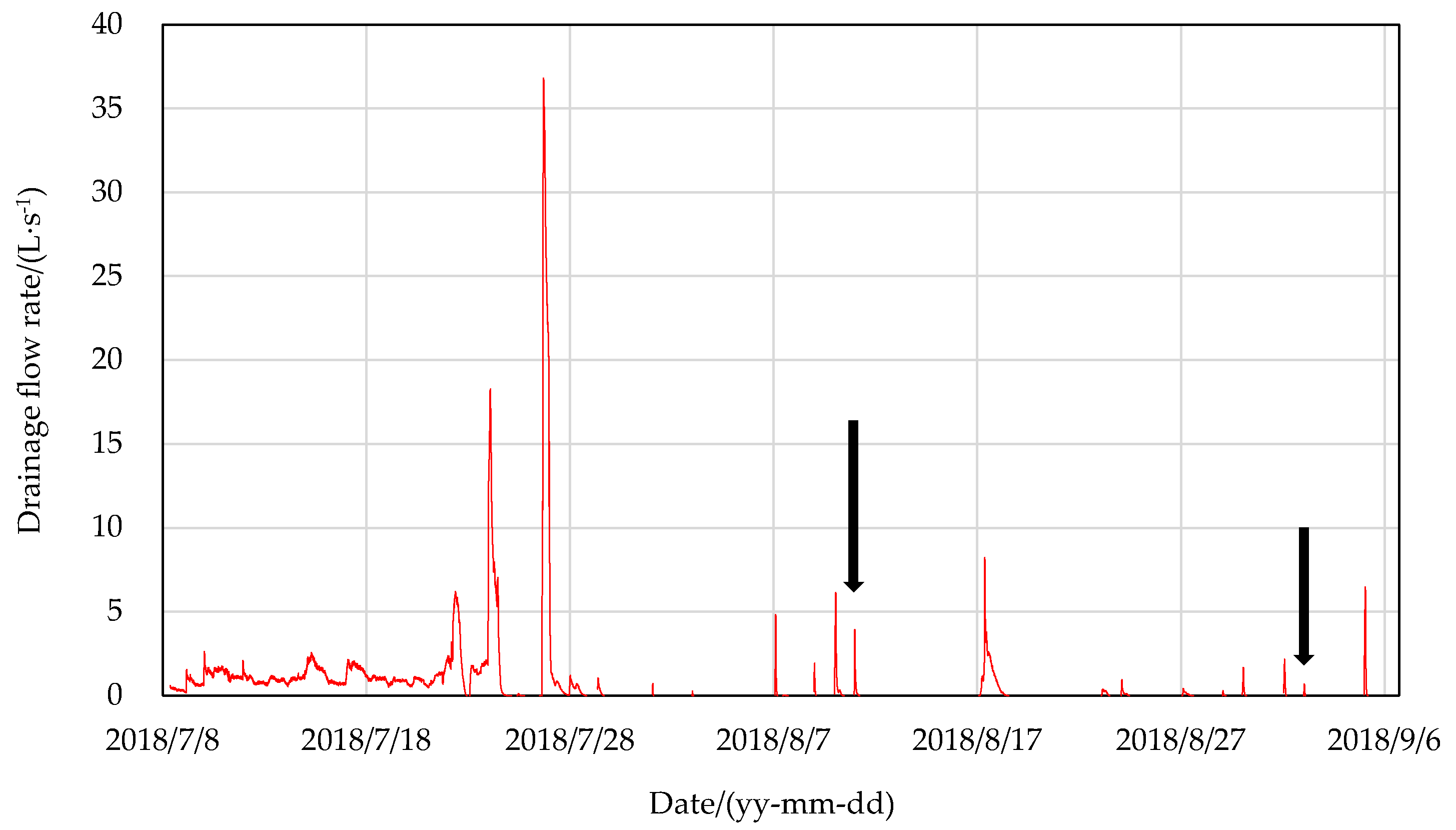
3.1. Drainage Process at the Field Edge during the Rice Growing Season

Figure 2 shows the drainage process during the rice growing season in 2018. The high flow rate events occurred with low frequency but showed a pulse-type feature. The drainage flow rate exceeded 5 L s−1 for only six times, which normally lasted for less than 1 h. Meanwhile, the main large drainage pulses did not occur during the insecticide application periods. The year 2018 was a wet year with an annual precipitation of 1156 mm. Drainage occurred during the two application events in 2018, but the drainage volume was extremely different (15.8 and 2.1 m3 accounting for 0.49% and 0.06% of the total monitored drainage volume, respectively).

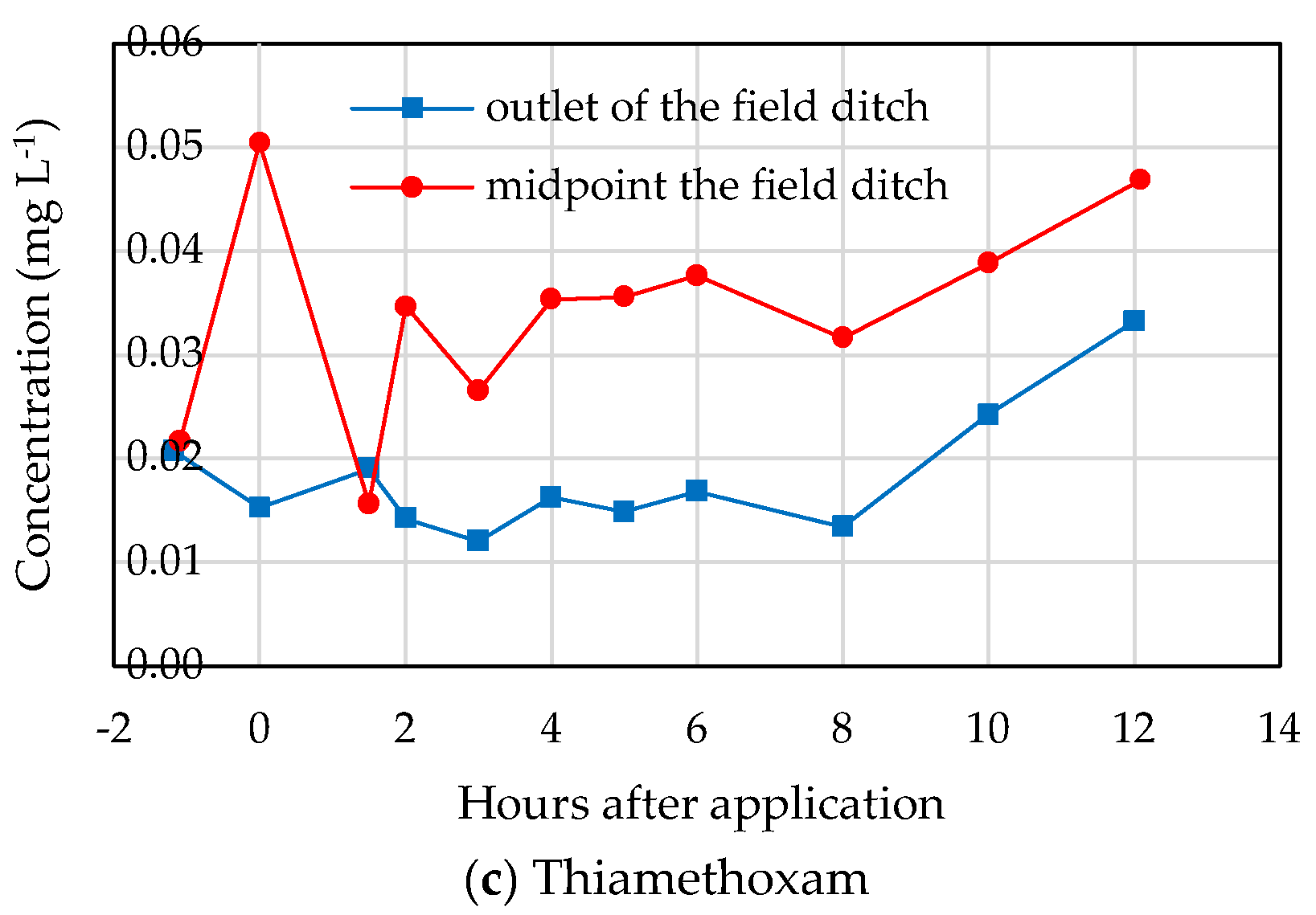
3.2. Insecticide Concentration Variations in Different Waters

The recoveries of CPF, THM and ABM were 81.2–137.8%, 91.6–148.4% and 56.9–149.1%, respectively. For all the surface water samples, the maximum relative error between two duplicate concentration measurements was 20.41%, indicating that the measurement accuracy was acceptable. With respect to the background level measurements, THM was detected at the ditch outlet, field surface water and groundwater, while CPF and ABM were not detected in all samples. For convenience, the abbreviation “cinsecticide-sampling point” was used to represent the measured concentrations of a certain insecticide at a certain sampling point: “d” denotes field ditch; “o” denotes outlet of the ditch; “m” denotes midpoint of the ditch; “p” denotes paddy surface water; “g” denotes paddy groundwater.
Figure 3 presents the measured insecticide concentrations in the field ditch and paddy surface water within 24 h after application. Much lower concentrations were observed thereafter for CPF, which are listed in Table 2, while ABM had not been detected since 36 h after application. cCPF-g was detected in only four of the groundwater samples: 0.001 (0 h), 0.002 (2 h), 0.0012 (4 h) and 0.0006 mg L−1 (36 h).
As shown in Figure 3a,b, three significant features of the behavior of three insecticides could be summarized: (1) cCPF-o was higher than cCPF-m (with one exception at 1 h after application), while cTHM-o was lower than cTHM-m, and cCPF-d was generally higher than cCPF-p; (2) two evident peaks appeared within 5 h after application, and a much less evident peak appeared at 12 h for both CPF and ABM, while no evident peaks were observed for THM; (3) at the two sampling points in the ditch, variation trends of cCPF-d differed with each other during the outflow period, while variation trends of cTHM-d were more similar.
Three co peaks could be observed both for CPF and ABM; the first two CPF peaks were more evident and similar: 0.329 mg L−1 (maximum value of all the measured CPF concentrations) at 2 h and 0.328 mg L−1 at 5 h after application. Only one cCPF-m peak could be observed (0.170 mg L−1 at 4 h) after application. As for ABM, only the second cABM-o peak (0.0046 mg L−1 at 5 h) was fairly evident. cCPF-o and cABM-o fluctuated within the first 12 h after application and decreased to the initial level (0 h) at 24 h. cCPF-d was higher than cCPF-p within 8 h after application; cCPF-o was 1.8–22.3 (11.0 in average) times that of cCPF-p, and cCPF-m was 1.2–17.0 (6.2 in average) times that of cCPF-p during this period. Similar to ABM, cCPF-o was higher than cCPF-m except at one point (0 h). Within 12 h after application, cCPF-d at the two sampling points showed an opposite variation trend during the six time intervals. cCPF-p varied in a relatively narrow range (0.010–0.050 mg L−1) with two less evident peaks (0.050 mg L−1 at 1 h and 0.042 mg L−1 at 10 h after application). Measured cCPF was significantly lower after 24 h of application (Table 2). The time period of 12–24 h after application can be roughly considered as the threshold that divided the high and low concentration levels; the average cCPF-o, cCPF-m and cCPF-p during the high-level period (0–12 h) were, respectively, 10.4, 7.9 and 3.0 folds of those during the low-level period (24–72 h).
The observed THM behavior, as shown in Figure 3c, exhibited a totally different pattern from CPF and ABM. From the aspect of spatial variation, cTHM-m was higher than cTHM-o, except at 1.5 h after application. The average cTHM-m was 0.8–3.3 (2.0 in average) folds of cTHM-o. Interestingly, the variation trends of cTHM-m and cTHM-o were opposite to each other from −1 to 2 h, and they varied with the same trend thereafter. The temporal variations showed no evident concentration peaks within 12 h after application; cTHM-d showed a steadily increasing trend from 8 to 12 h after application. The maximum value of cTHM-d (0.0504 mg L−1) was only a very small fraction (1.2 × 10⁻⁵) of the THM solubility in water (Table 1), which was quite different from CPF (0.31) and ABM (0.23).

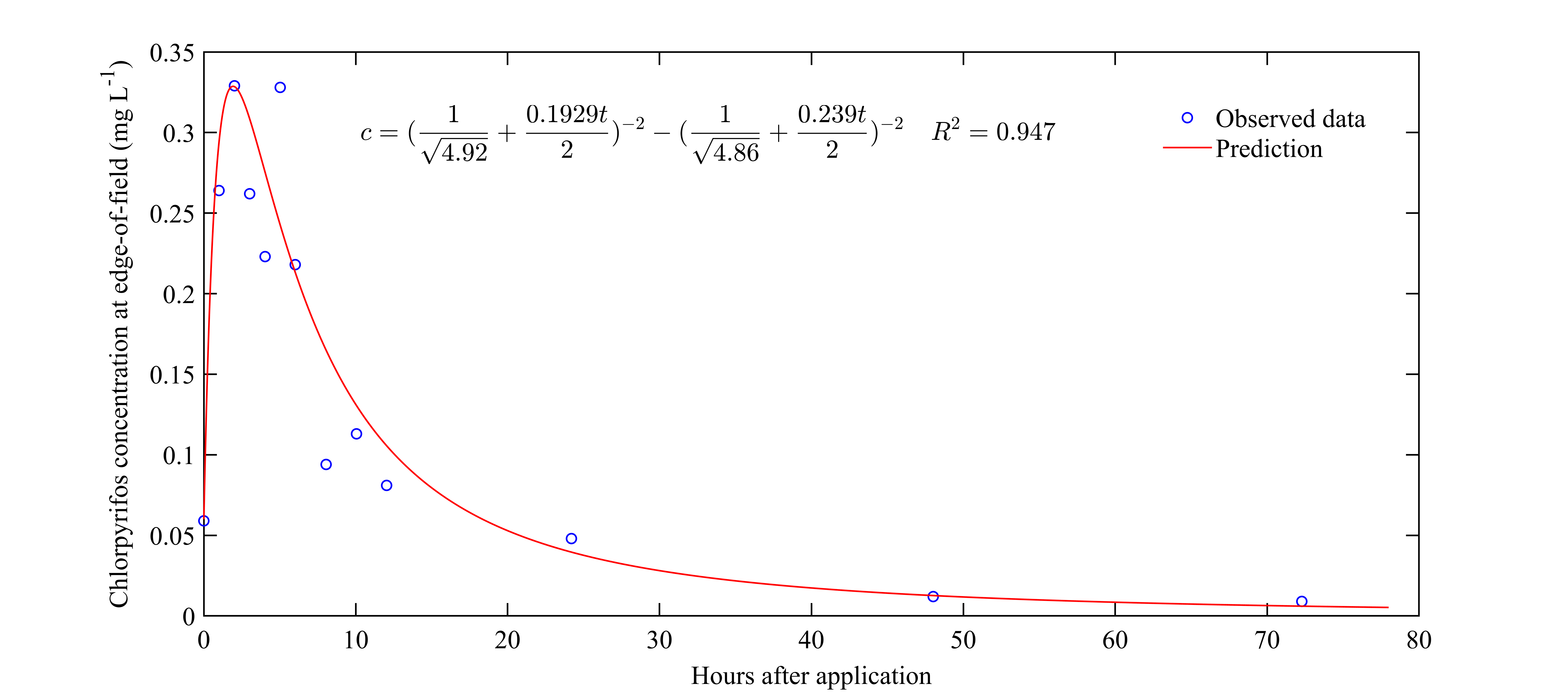
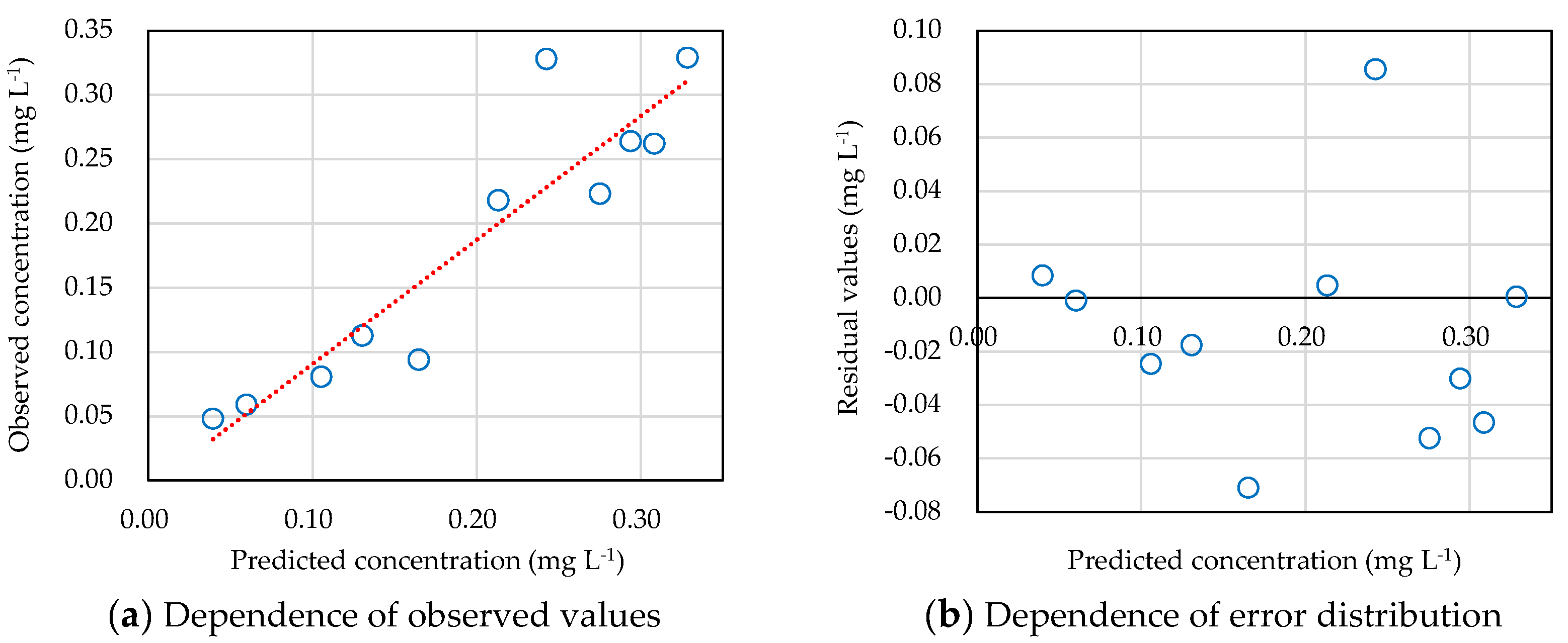
3.3. Kinetic Model to Predict Insecticide Concentration Variations

The conventional first-order kinetics as well as other currently available models [22] failed to well describe the observed edge-of-field insecticide concentration variations in this study. We tried all the possible combinations (plus and minus) of the models in [22] and eventually found that a combined 1.5–1.5-order kinetic model (i.e., a 1.5-order kinetic equation minus another one) was most appropriate for fitting cCPF-o (data point of 36 h was removed), as follows:
c = ( 1 4.92 + 0.1929 t 2 ) 2 ( 1 4.86 + 0.239 t 2 ) 2
The calculated VRE was 19.84% (0.16–75.43% for all the data points in Figure 4), and VAE was 0.0266 mg L−1 (0.0004–0.0854 mg L−1). With the proposed model, the relative error of the predicted peak concentration was −0.16%, and the absolute error was slightly less than 0.001 mg L−1. If the peak concentration was taken as the initial point (1.9 h after application), the calculated dissipation half-lives of CPF (the time after which cCPF decreased to half of the initial concentration) at the outlet of the ditch were 6.2, 6.6, 9.0, 12.6, 17.7 and 25.1 h, respectively.
Results of dependence of observed chlorpyrifos concentration and error distribution on the predicted values provided by the combined 1.5–1.5-order kinetic model are exhibited in Figure 5 [1]. The data points in Figure 5a are on the opposite sides of the red straight line, indicating the errors with a random spread (Figure 5b). These errors were insignificant in value. It can thus be concluded that the systematic errors were absent in the prediction of chlorpyrifos concentration based on the proposed kinetic model. It should be noted that the proposed kinetic model predicted the concentrations of CPF well, but not for THM and ABM. This may be caused by the particular property (high volatility) of CPF, which requires further exploration in the future.

3.4. Estimated Insecticide Loads

Figure 6 presents the calculated quarter-hourly loads of CPF and ABM exported from the ditch outlet. The quarter-hourly load of CPF peaked to 88.4 mg during the second quarter-hour period (0.25–0.50 h after application). The areal load of CPF was 656.8 mg ha−1 during the whole runoff event (lasting for 5 h) in the field ditch after insecticide application, which is equal to 3.11 g ha−1 d−1. The quarter-hourly load of ABM peaked to 1.09 mg during the first quarter-hour (0–0.25 h after application). The areal load of ABM was 7.43 mg ha−1 during the whole runoff event in the field ditch after application, which is equal to 0.035 g ha−1 d−1.
The runoff ratios of CPF and ABM exports in the field ditch (amount of insecticides exports during runoff period over the applied amount) were 0.17% and 0.069%, respectively. The cumulative areal loads of CPF and ABM during the first hour after application were, respectively, 336.9 and 3.9 mg ha−1, indicating that more than half of the CPF (51.3%) and ABM (53.0%) load was exported within 1 h after application.
Only one water sample was collected during the outflow period for THM. The calculated THM loading rate (mass of THM discharged with drainage water at the ditch outlet per unit time) when the water sample was collected was 0.003 mg s−1 (0.011 g h−1). It is worth noting that the flow discharge at the ditch outlet peaked at 45 min and 2 h, respectively, after the beginning of the first and second insecticide application events. The uncertain phase relationship between flow discharge and insecticide concentration peaks could have a significant influence on the feature of edge-of-field insecticide load peaks.

4. Discussion

4.1. Drainage Feature during the Pest-Control Irrigation Period

The water level of the field ditch was relatively steady, leading to continuous outflow before 22 July. The outflow stopped for the first time on 23 July, after which the water level of the field ditch varied rapidly within a wide scope. It is indicated that the paddy field was irrigated slightly but frequently. The rice entered into the jointing booting stage as well as the beginning of the pest-control period since 22 July. The volume of irrigation and drainage became large due to the need for rice growth. The water level of the field ditch thus varied noticeably, and the outflow exhibited a pulse-type drainage feature. Twenty outflow events occurred after 23 July, which lasted from several hours to 2 d. During the two pest-control irrigation events, the outflow lasted for near 6.8 h on 11 August, while it lasted for only 2.5 h on 2 September. In summary, the pulse-type drainage features during the pest-control irrigation period can be summarized as short duration (normally less than 1 d), large flow rate (as large as 4 L·s−1), frequent occurrence (20 times during a 40-d period) and long time interval (as long as 5 d). These drainage features provide a hydrological condition prone to the loss of contamination, such as applied insecticides.

4.2. Factors Affecting the Field-Scale Insecticide Behavior

4.2.1. Effect of Physico-Chemical Properties of Insecticides

The distinct behavior observed for CPF and THM in the ditch can be explained by their different physico-chemical properties. Neonicotinoids with lower Henry’s constant and vapor pressure have low potential of volatilization and may be briefly present in gaseous form during spray applications [28]. The Henry’s constant and vapor pressure of CPF are higher than those of THM by nine and six orders of magnitude, respectively (Table 1); thus, CPF contained in the paddy surface water migrated to the ditch water with the effects of volatilization and deposition during and after application rather than THM. Additionally, the leachability to groundwater significantly increases with increasing water solubility and with decreasing octanol–water partition coefficient. The fact that no evident THM concentration peaks were observed shortly after application could be attributed to the high leachability of THM to groundwater [29] and the consequent different transport pathway from CPF and ABM. More THM contained in the groundwater would slowly travel into the adjacent ditch with shallow subsurface drainage, leading to a THM peak occurring at a longer time after application.

4.2.2. Effect of the Primary and Secondary Drift

Since no surface runoff from the paddy field to the field ditch occurred during the sampling procedure, it is indicated that insecticide drift and atmospheric deposition predominantly contributed to the high CPF concentration levels in the field ditch compared with the paddy surface water. According to the weather data recordings, east and northeast winds prevailed on the first day of both sampling events, and the wind drift effect elevated insecticide concentrations in the field ditch. Das et al. [30] revealed that CPF concentration in air decreased rapidly within 1 d after application, which exhibited a similar trend with the observed CPF concentration in paddy drainage water. This indicates that the CPF contamination in drainage water should be briefly attributed to the atmospheric deposition after application.
cCPF-m was higher than cCPF-o within 1 h after application (the same for ABM), but a different spatial distribution of CPF was observed afterwards. This phenomenon cannot be simply interpreted by wind drift, as there were no significant variations of wind direction during these two periods. The different characteristics between the primary and secondary drift were accountable for the observed insecticide behavior [31]. It should be noted that insecticides were sprayed from west to east paddy plots, and sprayers traveled in each plot in a vertical direction, which means they got close to the upstream section of the ditch to the south of the paddy fields several times during spray application. Consequently, the upstream section would have higher potential of being directly contaminated by insecticide droplets during application (primary drift). When the application ended, the effect of wind drift (secondary drift) added up to the CPF concentrations along the ditch, and thus cCPF-o was higher than cCPF-m afterwards.

4.2.3. Deposition and Volatilization at the Air–Water Interface

The hydrolysis and photolysis DT50 of CPF (Table 1) were much longer than the calculated half-life (6.2 h) of cCPF-o during the high concentration level, indicating that the effect of photolysis and hydrolysis on the disappearance of CPF from the ditch water was negligible [19,32]. However, a sharp decline of cCPF-o still appeared after the two peaks. Giesy et al. [33] reported the relatively fast initial volatilization of applied CPF during the first 12 h after application. This was the case even though with a relatively high Henry’s constant and vapor pressure values, secondary insecticide drift intensity of CPF declined sharply after application [31,34]. In summary, the observed fluctuation of cCPF-o and cCPF-m should be the result of the comprehensive effects of deposition and volatilization through the air–water interface.
Zivan et al. [31] observed that weak winds on the night after application resulted in a secondary peak (three-fold increase during low concentration level period) in air concentrations of CPF. This coincides with the phenomenon observed in this study: cCPF-o and cCPF-p increased by 20.2% and 61.5%, respectively, in the 10–12 h period after application. It is fairly reasonable to postulate that this was caused by the increased atmospheric CPF concentration.
As observed, two consecutive rainfall events occurred in 40.5–41.5 h (6.35 mm) and 45.0–46.5 h (2.29 mm) after application. They were the drivers of the cCPF-m increase (69.4%) at 36 and 48 h after application, probably from two aspects: (1) wet deposition (deposition of insecticides in rain) sending CPF from air to ditch water directly [35]; and (2) wetter soil stimulating volatilization of CPF in the paddy surface water (the increased air concentration may have deposited more into the ditch water).

4.3. Insights from High-Frequency Monitoring of Insecticides

The peak concentration is a significant parameter for ecological risk assessment of pesticides [36]. We could take the case of CPF as an example. The maximum, median and mean values of cCPF-o (0–12 h after application) were 0.329, 0.221 and 0.197 mg L−1, respectively, which could be calculated from the results exhibited in Figure 3a. If the data points at 1, 3 and 5 h were removed (the shortest sampling interval would be 2 h), the maximum, median and mean values would be 0.329, 0.113 and 0.160 mg L−1, respectively. With the shortest sampling interval of 4 h, the values would be 0.223, 0.088 and 0.114 mg L−1, respectively. Therefore, less frequent sampling (from shortest sampling intervals of 1, 2 and 4 h) would underestimate the maximum (by 0% and 32.2%), median (by 48.9% and 60.2%) and mean (by 18.8% and 42.1%) concentrations shortly after application.
In existing studies, water samples were normally taken immediately after and/or in several hours of pesticide application, which were assumed to represent concentration peaks during high-level concentration periods. Afterwards, samples were usually taken at time intervals of not shorter than 1 d [15,17,37]. As we demonstrated with our observations, large concentration variations may exist after spray application; occasional and low frequency sampling may probably depict the insecticide concentration dynamics poorly [6]. The cCPF peak reported by Duffner et al. [38] was less than 1/20 of the observed cCPF peak in this study. The peak observed with sampling intervals of more than 2 d might be higher if high-frequency monitoring was conducted. As indicated in this study, high-frequency monitoring of insecticides should better be more frequently used to obtain a more scientific knowledge of the behavior of insecticides and their actual adverse impacts on the environment [20].
According to the high-frequency monitoring results of CPF and ABM, concentrations of these two insecticides at the outlet of the ditch both declined to the concentration level immediately post application. Hence, it is recommended that controlled drainage be implemented for at least 1 d post application to prevent the loss of insecticides during the high-level export period. Periodical irrigation is applied in paddies for both the needs of the physiological and ecological water requirements of rice. Specifically, refreshing of the paddy surface water could ensure adequate dissolved oxygen that is beneficial for rice growth [39] and prevent the potential damage of heat stress. Consequently, the rigid demand of drainage in paddies during the whole rice growing season and the controlled drainage demand during and after pest-control irrigation for preventing loss of insecticides result in a contradiction. High-frequency monitoring of insecticides could capture the whole process of insecticide peaks and thus obtain a more accurate time period of high-level insecticide export. On the basis of this, we could scientifically determine the duration of controlled drainage to achieve a balance.

5. Conclusions

Based on field-scale monitoring of the drainage process and three insecticides in a rice paddy and an adjacent field ditch, we observed that the pulse-type drainage during the pest-control irrigation period exhibited the following features: short duration (normally less than 1 d), large flow rate (as large as 4 L s−1), frequent occurrence (20 times during a 40-d period) and long time interval (as long as 5 d). Edge-of-field export of insecticides with higher Henry’s constant and vapor pressure exhibited strong temporal pulse-type features. Concentrations of chlorpyrifos and abamectin peaked quickly (within several hours) post application in the field ditch; more than half of chlorpyrifos and abamectin loads were exported within merely 1 h after application. From the perspective of spatial variation of insecticides, chlorpyrifos concentrations in the ditch were much higher than those in paddy surface water or groundwater within several hours after application; thus more attention should be paid to the high contamination potential in field ditches surrounding rice paddies. Chlorpyrifos concentrations increased along the ditch due to insecticide drift, which could be explained by primary and the secondary drift. Deposition and volatilization of chlorpyrifos have a much more significant effect on its concentration variation in the ditch than degradation shortly after application. Rainfall-induced small concentration peak in the ditch occurred 1.5–2 d after application, but it was much less evident than the peaks occurring right after application. The proposed kinetic model described the concentration variation characteristic of chlorpyrifos at edge-of-field reasonably well by capturing both the rising and falling limbs. Although the determination of parameters used in this model may be time-consuming because of the complexity of the equation form. The field-scale high-frequency monitoring of insecticides that is able to detect accurate concentration peaks could provide valuable information for water management practice and ecological risk assessment.

Author Contributions

Conceptualization, Z.J. and C.C.; Methodology, C.C.; Formal analysis, C.C.; Investigation, C.C. and J.Z.; Writing—original draft preparation, C.C.; Writing—review and editing, W.L. and Z.J.; Funding acquisition, Z.J. All authors have read and agreed to the published version of the manuscript.

Funding

This study was funded by the National Natural Science Foundation of China (No. 51979239), the Water Conservancy Science and Technology Project of Jiangsu Province, China (No. 2017052).

Conflicts of Interest

The authors declare no conflict of interest.

References

  1. Astaykina, A.; Streletskii, R.; Maslov, M.; Kazantseva, S.; Karavanova, E.; Gorbatov, V. Novel pesticide risk indicators for aquatic organisms and earthworms. Agronomy 2020, 10, 1070. [Google Scholar] [CrossRef]
  2. Kosamu, I.; Kaonga, C.; Utembe, W. A critical review of the status of pesticide exposure management in Malawi. Int. J. Environ. Res. Public Health 2020, 17, 6727. [Google Scholar] [CrossRef] [PubMed]
  3. Sun, C.; Chen, L.; Zhai, L.; Liu, H.; Jiang, Y.; Wang, K.; Jiao, C.; Shen, Z. National assessment of spatiotemporal loss in agricultural pesticides and related potential exposure risks to water quality in China. Sci. Total Environ. 2019, 677, 98–107. [Google Scholar] [CrossRef] [PubMed]
  4. Chowdhury, M.A.Z.; Banik, S.; Uddin, B.; Moniruzzaman, M.; Karim, N.; Gan, S.H. Organophosphorus and carbamate pesticide residues detected in water samples collected from paddy and vegetable fields of the Savar and Dhamrai Upazilas in Bangladesh. Int. J. Environ. Res. Public Health 2012, 9, 3318–3329. [Google Scholar] [CrossRef] [Green Version]
  5. Furihata, S.; Kasai, A.; Hidaka, K.; Ikegami, M.; Ohnishi, H.; Goka, K. Ecological risks of insecticide contamination in water and sediment around off-farm irrigated rice paddy fields. Environ. Pollut. 2019, 251, 628–638. [Google Scholar] [CrossRef]
  6. Stehle, S.; Knäbel, A.; Schulz, R. Probabilistic risk assessment of insecticide concentrations in agricultural surface waters: A critical appraisal. Environ. Monit. Assess. 2013, 185, 6295–6310. [Google Scholar] [CrossRef]
  7. Ashauer, R.; Brown, C.D. Highly time-variable exposure to chemicals—Toward an assessment strategy. Integr. Environ. Assess. Manag. 2013, 9, e27–e33. [Google Scholar] [CrossRef] [PubMed]
  8. Rasmussen, J.J.; Wiberg-Larsen, P.; Kristensen, E.A.; Cedergreen, N.; Friberg, N. Pyrethroid effects on freshwater invertebrates: A meta-analysis of pulse exposures. Environ. Pollut. 2013, 182, 479–485. [Google Scholar] [CrossRef] [Green Version]
  9. Wieczorek, M.V.; Bakanov, N.; Bilancia, D.; Szöcs, E.; Stehle, S.; Bundschuh, M.; Schulz, R. Structural and functional effects of a short-term pyrethroid pulse exposure on invertebrates in outdoor stream mesocosms. Sci. Total Environ. 2018, 610, 810–819. [Google Scholar] [CrossRef]
  10. Rothstein, E.; Steenhuis, T.S.; Peverly, J.H.; Geohring, L.D. Atrazine fate on a tile drained field in northern New York: A case study. Agric. Water Manag. 1996, 31, 195–203. [Google Scholar] [CrossRef]
  11. Anyusheva, M.; Lamers, M.; La, N.; Nguyen, V.V.; Streck, T. Fate of pesticides in combined paddy rice-fish pond farming systems in Northern Vietnam. J. Environ. Qual. 2012, 41, 515–525. [Google Scholar] [CrossRef] [PubMed] [Green Version]
  12. Phong, T.K.; Yoshino, K.; Hiramatsu, K.; Harada, M.; Inoue, T. Pesticide discharge and water management in a paddy catchment in Japan. Paddy Water Environ. 2010, 8, 361–369. [Google Scholar] [CrossRef]
  13. Sangchan, W.; Hugenschmidt, C.; Ingwersen, J.; Schwadorf, K.; Thavornyutikarn, P.; Pansombat, K.; Streck, T. Short-term dynamics of pesticide concentrations and loads in a river of an agricultural watershed in the outer tropics. Agric. Ecosyst. Environ. 2012, 158, 1–14. [Google Scholar] [CrossRef]
  14. Watanabe, H.; Nguyen, M.H.T.; Souphasay, K.; Vu, S.H.; Phong, T.K.; Tournebize, J.; Ishihara, S. Effect of water management practice on pesticide behavior in paddy water. Agric. Water Manag. 2007, 88, 132–140. [Google Scholar] [CrossRef]
  15. Zhang, X.; Shen, Y.; Yu, X.Y.; Liu, X.J. Dissipation of chlorpyrifos and residue analysis in rice, soil and water under paddy field conditions. Ecotoxicol. Environ. Saf. 2012, 78, 276–280. [Google Scholar] [CrossRef]
  16. Thuyet, D.Q.; Watanabe, H.; Motobayashi, T.; Ok, J. Behavior of nursery-box-applied fipronil and its sulfone metabolite in rice paddy fields. Agric. Ecosyst. Environ. 2013, 179, 69–77. [Google Scholar] [CrossRef]
  17. Fu, Y.; Liu, F.; Zhao, C.; Zhao, Y.; Liu, Y.; Zhu, G. Distribution of chlorpyrifos in rice paddy environment and its potential dietary risk. J. Environ. Sci. 2015, 35, 101–107. [Google Scholar] [CrossRef]
  18. Tsochatzis, E.D.; Tzimou-Tsitouridou, R.; Menkissoglu-Spiroudi, U.; Karpouzas, D.G.; Katsantonis, D. Laboratory and field dissipation of penoxsulam, tricyclazole and profoxydim in rice paddy systems. Chemosphere 2013, 91, 1049–1057. [Google Scholar] [CrossRef]
  19. Tang, X.Y.; Yang, Y.; McBride, M.B.; Tao, R.; Dai, Y.N.; Zhang, X.M. Removal of chlorpyrifos in recirculating vertical flow constructed wetlands with five wetland plant species. Chemosphere 2019, 216, 195–202. [Google Scholar] [CrossRef]
  20. Lefrancq, M.; Jadas-Hécart, A.; La Jeunesse, I.; Landry, D.; Payraudeau, S. High frequency monitoring of pesticides in runoff water to improve understanding of their transport and environmental impacts. Sci. Total Environ. 2017, 587, 75–86. [Google Scholar] [CrossRef] [Green Version]
  21. Joseph, A.; Ort, C.; Brien, D.S.O.; Lewis, S.E.; Davis, A.M.; Mueller, J.F. Understanding the uncertainty of estimating herbicide and nutrient mass loads in a flood event with guidance on estimator selection. Water Res. 2018, 132, 99–110. [Google Scholar] [CrossRef] [Green Version]
  22. Fantke, P.; Juraske, R. Variability of pesticide dissipation half-lives in plants. Environ. Sci. Technol. 2013, 47, 3548–3562. [Google Scholar] [CrossRef] [PubMed]
  23. Akan, A.O. Open Channel Hydraulics, 1st ed.; Elsevier: Oxford, UK, 2006; ISBN 9780750668576. [Google Scholar]
  24. Jia, Z.; Chen, C.; Luo, W.; Zou, J.; Wu, W.; Xu, M.; Tang, Y. Hydraulic conditions affect pollutant removal efficiency in distributed ditches and ponds in agricultural landscapes. Sci. Total Environ. 2019, 649, 712–721. [Google Scholar] [CrossRef]
  25. Chen, C.; Jia, Z.; Luo, W.; Hong, J.; Yin, X. Efficiency of different monitoring units in representing pollutant removals in distributed ditches and ponds in agricultural landscapes. Ecol. Indic. 2020, 108, 105677. [Google Scholar] [CrossRef]
  26. Lewis, K.A.; Tzilivakis, J.; Warner, D.J.; Green, A. An international database for pesticide risk assessments and management. Hum. Ecol. Risk Assess. 2016, 22, 1050–1064. [Google Scholar] [CrossRef] [Green Version]
  27. Joo, M.; Raymond, M.A.A.; McNeil, V.H.; Huggins, R.; Turner, R.D.R.; Choy, S. Estimates of sediment and nutrient loads in 10 major catchments draining to the Great Barrier Reef during 2006–2009. Mar. Pollut. Bull. 2012, 65, 150–166. [Google Scholar] [CrossRef]
  28. Bonmatin, J.M.; Giorio, C.; Girolami, V.; Goulson, D.; Kreutzweiser, D.P.; Krupke, C.; Liess, M.; Long, E.; Marzaro, M.; Mitchell, E.A.; et al. Environmental fate and exposure; neonicotinoids and fipronil. Environ. Sci. Pollut. Res. 2015, 22, 35–67. [Google Scholar] [CrossRef]
  29. Akay Demir, A.E.; Dilek, F.B.; Yetis, U. A new screening index for pesticides leachability to groundwater. J. Environ. Manag. 2019, 231, 1193–1202. [Google Scholar] [CrossRef]
  30. Das, S.; Hageman, K.J.; Taylor, M.; Michelsen-Heath, S.; Stewart, I. Fate of the organophosphate insecticide, chlorpyrifos, in leaves, soil, and air following application. Chemosphere 2020, 243, 125194. [Google Scholar] [CrossRef]
  31. Zivan, O.; Segal-Rosenheimer, M.; Dubowski, Y. Airborne organophosphate pesticides drift in Mediterranean climate: The importance of secondary drift. Atmos. Environ. 2016, 127, 155–162. [Google Scholar] [CrossRef]
  32. Mazanti, L.; Rice, C.; Bialek, K.; Sparling, D.; Stevenson, C.; Johnson, W.E.; Kangas, P.; Rheinstein, J. Aqueous-phase disappearance of atrazine, metolachlor, and chlorpyrifos in laboratory aquaria and outdoor macrocosms. Arch. Environ. Contam. Toxicol. 2003, 44, 67–76. [Google Scholar] [CrossRef] [PubMed]
  33. Giesy, J.P.; Solomon, K.R. Ecological Risk Assessment for Chlorpyrifos in Terrestrial and Aquatic Systems in the United States. In Reviews of Environmental Contamination and Toxicology; Springer: Cham, Switzerland, 2014; pp. 35–76. [Google Scholar]
  34. Zivan, O.; Bohbot-Raviv, Y.; Dubowski, Y. Primary and secondary pesticide drift profiles from a peach orchard. Chemosphere 2017, 177, 303–310. [Google Scholar] [CrossRef] [PubMed]
  35. Potter, T.L.; Coffin, A.W. Assessing pesticide wet deposition risk within a small agricultural watershed in the Southeastern Coastal Plain (USA). Sci. Total Environ. 2017, 580, 158–167. [Google Scholar] [CrossRef] [PubMed] [Green Version]
  36. Pereira, A.S.; José Cerejeira, M.; Daam, M.A. Ecological risk assessment of imidacloprid applied to experimental rice fields: Accurateness of the RICEWQ model and effects on ecosystem structure. Ecotoxicol. Environ. Saf. 2017, 142, 431–440. [Google Scholar] [CrossRef]
  37. Teló, G.M.; Marchesan, E.; Zanella, R.; De Oliveira, M.L.; Coelho, L.L.; Martins, M.L. Residues of fungicides and insecticides in rice field. Agron. J. 2015, 107, 851–863. [Google Scholar] [CrossRef]
  38. Duffner, A.; Ingwersen, J.; Hugenschmidt, C.; Streck, T. Pesticide transport pathways from a sloped litchi orchard to an adjacent tropical stream as identified by hydrograph separation. J. Environ. Qual. 2012, 41, 1315–1323. [Google Scholar] [CrossRef]
  39. Feng, Z.; Chunmei, X.; Weijian, Z.; Xiufu, Z.; Fengbo, L.; Jianping, C.; Danying, W. Effects of rhizosphere dissolved oxygen content and nitrogen form on root traits and nitrogen accumulation in rice. Rice Sci. 2011, 18, 304–310. [Google Scholar] [CrossRef]
Figure 1. Schematic diagram of the study area: (a) three-dimensional view derived from satellite image; (b) on-site view. The distance between the two sampling points at the field ditch is around 93 m. Agronomy 10 01615 i001 boundary of the stud y area, Agronomy 10 01615 i002 position and angle of view of Figure 1b, Agronomy 10 01615 i003 field ditch, Agronomy 10 01615 i004 weather station. Agronomy 10 01615 i005 sampling point at the midpoint of the field ditch, Agronomy 10 01615 i006 v-notch weir (sampling point at the outlet of the field ditch), Agronomy 10 01615 i007 sampling point of the paddy surface water, Agronomy 10 01615 i008 90-cm depth well (sampling point of the paddy groundwater).
Agronomy 10 01615 g001
Figure 2. Drainage process of the field ditch from 8 July to 7 September 2018. The black arrows denote the time of insecticide applications.
Agronomy 10 01615 g002
Figure 3. Measured insecticide concentrations at the outlet and midpoint of the field ditch and paddy surface water during or within 24 h after spray applications: (a) chlorpyrifos; (b) abamectin; (c) thiamethoxam.
Agronomy 10 01615 g003aAgronomy 10 01615 g003b
Figure 4. Fitted curve of the combined 1.5–1.5-order kinetic model for the prediction of chlorpyrifos concentration at the outlet of the field ditch adjacent to paddy fields.
Agronomy 10 01615 g004
Figure 5. Analysis results of the dependence of (a) observed values and (b) error distribution on the predicted values.
Agronomy 10 01615 g005
Figure 6. Quarter-hourly and cumulative edge-of-field loads of (a) chlorpyrifos and (b) abamectin during the 5-h runoff event after spray application.
Agronomy 10 01615 g006
Table 1. Properties of the monitored insecticides obtained from PPDB and BPDB.
InsecticideSubstance GroupSolubility in Water (20 °C) (mg L−1)Henry’s Constant (25 °C)
(Pa m3 mol−1)
Vapor Pressure (25 °C)
(mPa)
Koc/Kfoc 3
(mL g−1)
Kow (log P) (20 °C, pH 7)Aqueous Hydrolysis DT50 (20 °C, pH 7) (d)Aqueous Photolysis DT50 (pH 7) (d)Soil Degradation DT50 (field) (d)
CPF 1Organophosphate1.050.4781.435509/39544.753.529.627.6
ABM 2Micro-organism derived0.0202.70 × 10−30.0037NA 4/66314.4Stable1.51
THM 1Neonicotinoid41004.70 × 10−106.60 × 10−656.2/NA 4−0.13Stable2.739
1 Obtained from the Pesticide Properties DataBase (PPDB) [26], which has been developed by the Agriculture and Environment Research Unit (AERU) at the University of Hertfordshire since 2007. 2 Obtained from the Bio-Pesticides DataBase (BPDB), which has been developed by AERU since 2011. 3 Koc (linear parameter) and Kfoc (non-linear parameter) both denote soil sorption coefficient. 4 NA: not available.
Table 2. Measured chlorpyrifos concentrations at the outlet and midpoint of the field ditch and paddy surface water at 36–72 h after the first spray application.
Hours after Application (h)364872
Outlet of the field ditch (mg L−1)0.00720.0120.0090
Midpoint of the field ditch (mg L−1)0.0200.0110.0066
Paddy surface water (mg L−1)0.0110.00960.0038
Publisher’s Note: MDPI stays neutral with regard to jurisdictional claims in published maps and institutional affiliations.

