Vegetable Crop Biomass Estimation Using Hyperspectral and RGB 3D UAV Data

Abstract

Remote sensing (RS) has been an effective tool to monitor agricultural production systems, but for vegetable crops, precision agriculture has received less interest to date. The objective of this study was to test the predictive performance of two types of RS data—crop height information derived from point clouds based on RGB UAV data, and reflectance information from terrestrial hyperspectral imagery—to predict fresh matter yield (FMY) for three vegetable crops (eggplant, tomato, and cabbage). The study was conducted in an experimental layout in Bengaluru, India, at five dates in summer 2017. The prediction accuracy varied strongly depending on the RS dataset used. For all crops, a good predictive performance with cross-validated prediction error < 10% was achieved. The growth stage of the crops had no significant effect on the prediction accuracy, although increasing trends of an underestimation of FMY with later sampling dates for eggplant and tomato were found. The study proves that an estimation of vegetable FMY using RS data is successful throughout the growing season. Different RS datasets were best for biomass prediction of the three vegetables, indicating that multi-sensory data collection should be preferred to single sensor use, as no one sensor system is superior.

1. Introduction

In the course of increasing urbanization, sustainable use of agricultural resources has become a pressing issue [1]. In developing countries, the population is projected to double by 2050 [2], and the occupation of arable land by cities will more than double. In combination with widespread malnutrition in such countries, especially in southern Asia, sustainable agriculture is necessary in order to increase food production [3]. For decades (e.g., [4,5]), remote sensing (RS) has been an effective tool to monitor agricultural production systems [6,7]. Particularly in countries with several cropping seasons per year, such as India, agricultural systems require multi-temporal RS data for a continuous evaluation of crop state and less ambiguous crop identification [8,9]. While crop identification can help to examine the effects of, for example, urbanization, on the farmers’ decisions to grow certain crops, an evaluation of the crop development, and thus biomass prediction, can enable evaluation of the intensity (i.e., fertilization and irrigation) of the agricultural practice. This information may allow one to manage fields more economically and be more efficient on small and large scales.

Intensive vegetable production, which is increasingly characterized by frequent nitrogen (N) fertilization [10], requires rapid and frequent assessment of crop status [11]. While precision agriculture (PA) for field crops was widely applied for two decades, it has a rather short history in horticulture [12,13]. The smaller field size and planting density, as well as the complex plant architecture, makes PA in horticulture complex [13]. Various sensor platforms, from terrestrial [14] and airborne [15] to satellite [16], have been used for investigating agro-environmental systems. Recently, unmanned aerial vehicles (UAV) have gained interest as platforms for collecting RS information from agricultural fields [15,17,18]. UAVs allow the collection of data from large areas (ranging from a few 100 m² for multi-rotor UAVs to approximately 200 ha for fixed-wing UAVs) in a highly repetitive manner, which makes them more independent from weather conditions than satellite or airborne platforms [19]. Another advantage of the UAV platform is their flexibility to carry various sensor systems, such as RGB cameras [15], multispectral sensors [20], and hyperspectral sensors [21], for monitoring crop parameters.

The availability of different sensor systems enables sensor fusion, i.e., the combination of datasets from two or more sensors with different characteristics [22]. Sensor fusion may allow a more holistic interpretation of the relationship between RS information and crop parameters. For example, the fusion of spectral reflectance information with data from an ultra-sound system showed an increased prediction performance for barley yield [23]. Other studies have shown an increased prediction performance of vegetation parameters, such as leaf area index (LAI) and biomass for various crops, such as maize [24], winter wheat [25], and soybean [20], when spectral and structural information (based on RADAR, LiDAR, or photogrammetric methods) were combined. In vegetable systems with a large structural variability, sensor fusion may improve yield estimations by remote sensing data.

With the development of new sensor systems, the amount of data generated has increased tremendously, creating demand for statistical methods which can handle a large quantity and often redundancy of data. Machine learning (ML) methods represent a group of empirical statistical methods able to handle huge amounts of data and intercorrelation of variables. Additionally, ML methods have frequently been used for modelling crop biomass with RS data (e.g., [15,20,23]). Various ML methods have been introduced in the RS community in recent years [26], e.g., partial least squares (PLS) regression [27] and random forest regression (RFR) [28]. Although a large variety of ML approaches are available, none of them consistently outperform the others, thus requiring that multiple methods be tested in order to find the optimal statistical model.

The primary objective of this study was to test the potential of two types of RS data—red-green-blue (RGB) data acquired by a UAV and terrestrial hyperspectral data—to predict the fresh matter yield (FMY) of three vegetable crops (eggplant, tomato, and cabbage). While in a former study [15] based on the same data collection, indirect allometric relationships between canopy height, modelled from 3D RGB UAV data with FMY data were used, in the present study, the derived point cloud information should be directly related to crop biomass. This direct approach should lead to improved FMY models, as the allometric relationship between biomass and canopy height is already suffering from noise and, thus, unexplained variation. Additionally, conversely to the previous study, a sensor data fusion approach with hyperspectral data is tested and evaluated. For establishing the empirical relationship, four different ML approaches were tested (partial least squares, support vector machines, random forest, and gradient boosting trees). The contribution and potential of data from each sensor individually (crop height values from the RGB dataset and spectral information from the hyperspectral dataset) and from both sensors fused together were evaluated. We hypothesized that sensor fusion improves the predictive performance of the models for all crops. Additionally, we expected that one ML approach alone will not deliver the optimal model all the time.

2. Methods

The data for this study were collected on the experimental farms of the University of Agricultural Science (UAS) in Bengaluru, India (12°58′20.79′′ N, 77°34′50.31′′ E, 920 asl) (Figure 1). The dominant soil types are Kandic Paleustalfs and Dystric Nitisols. The experimental site is characterized by a tropical climate with a distinct monsoon season from June to October. The mean annual temperature is 29.2 °C, with an average precipitation of 923 mm [29].

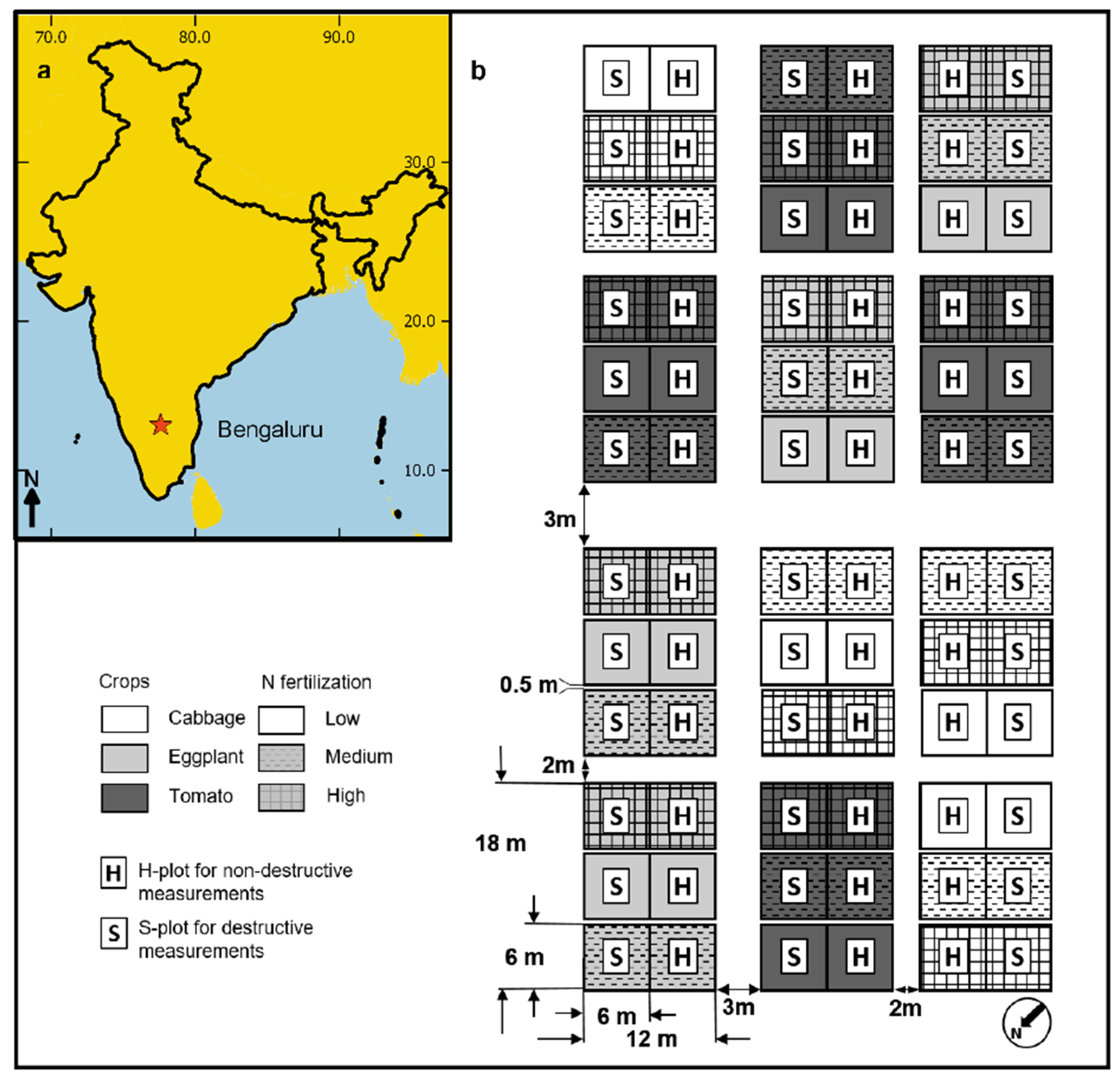
2.1. Field Experiment

The field experiment was established in 2016 and had a distinct rainy and dry season crop rotation. In the dry season (January to May), tomato (Solanum lycopersicum L.) (cultivar: NS-501), eggplant (Solanum melongena L.) (cultivar: Ankur), and cabbage (Brassica oleracea L.) (cultivar: Unnati) were grown (Figure 1b) with the use of a drip irrigation system. Twelve main plots (12 × 18 m) were arranged in a split-plot experiment. Each treatment was replicated four times (Figure 1b). Three subplots (6 × 12 m) with three levels of nitrogen (N) fertilizer were randomized within each main plot. A blanket application of phosphorus and potassium (40 kg P ha⁻¹ and 20, 24, and 50 kg K ha⁻¹ for eggplant, tomato, and cabbage) was given to all plots. Additionally, the mean N rate (50, 46, and 60 kg N ha⁻¹ as urea for eggplant, tomato, and cabbage, respectively) reflecting the recommended N dose in the region was applied for the medium dose plots. For the low- and high-dose plots, minus 50% and plus 50% of this dose was given, representing additional intensities typical of the region. Due to inaccuracies during the fertilization (fertilizers were not distributed evenly on the total plot area, but directly applied to individual plants), no nutrient deficiency was noticeable in either treatment. To allow for destructive measurements without disturbing neighboring plants, each subplot was divided equally into a destructive sub-subplot for biomass sampling (S-plot; Figure 1b) and a non-destructive sub-subplot (H-plot) for spectral measurements. The S- and H-plots were 6 × 6 m each. The layout was thus comprised of a total of 36 subplots (3 crops × 3 fertilizer treatments × 4 replicates).

2.2. Biomass Sampling

The total biomass (vegetative parts as well as fruits at later growth stages) was measured at five sampling dates between March and May 2017. Two randomly selected plant individuals were harvested (2 cm above the ground) in each S-plot (Figure 1b). These individuals can be considered as representative of the variation in the plot. Considering the number of plants in each plot (n = 100, 50, 50 for eggplant, tomato, and cabbage, respectively), two individuals was the compromise of not losing too many plants and reducing disturbances during the growth period. At each sampling date, the biomass (t ha⁻¹) was measured in the field using a balance. The total number of samples collected for each crop type was 60 (5 sampling dates × 3 fertilizer treatments × 4 replicates).

2.3. D UAV Point Cloud Data

At each sampling date, one RGB UAV flight for each plot was conducted using a DJI FC300X camera (focal length of 3.61 mm) mounted on DJI 3 Professional (DJI, Shenzhen, Guangdong, China). The same grid-wise flight plan was conducted for each plot using autopilot and the software Pix4D Capture (Pix4D SA, Lausanne, Switzerland). About 200 images (4000 × 3000 pixels) were taken during each flight for each plot, with an 80% forward and side overlap (Figure 2). The flight altitude ranged from 17 to 24 m which led to a variation in the mean ground resolution ranging from 6 to 8 mm per pixel. For a more detailed description of the flights, see [15]. In total, 60 flights (4 main plots × 3 crops × 5 sampling dates) were conducted. To reduce the effect of different geometries between the camera, sun, and vegetative surface between the flights, the same flight plan and approximately the same time of the day was selected for each sampling date. However, differences due to fluctuating areas of shadow and sun angel variations could not be avoided. As precise point cloud processing requires high spatial position accuracy, four permanent ground control points (GCPs) were measured in each main plot using a differential GPS (Trimble Inc., Sunnyvale, CA, USA) with a spatial accuracy of ~5 cm. These GCPs were subsequently used for georeferencing, geo-correction, and co-registration of the images. The GCPs were restricted to the corners of the plot due to practical reasons during the field season, in which standard agricultural practices prohibited the use of GCPs within each plot. This sparse GCP density potentially led to a degraded spatial accuracy [30]. Point cloud data were derived from the UAV RGB images using the structure-from-motion algorithm from the software Photoscan Pro (AgiSoft LLC, St. Petersburg, Russia). The procedures are comprised of a feature extraction process combined with a bundle adjustment of the images [31,32]. Applying a multi-view stereo matching algorithm, a dense point cloud was generated [33,34]. The detailed procedure for the dense point cloud creation is described in [15]. For each point of the point cloud, the red and green information was used to calculate the Green-Red Vegetation Index (GRVI) (Equation (1)) [5].

$$GRVI=\frac{\mathrm{Green}-\mathrm{Red}}{\mathrm{Green}+\mathrm{Red}}$$

(1)

Following the procedure described in [15], the GRVI was used for differentiating points representing ground and vegetation using a k-means classification. With the resulting ground points, a digital elevation model (DEM) was created using a Delaunay triangulation with a spatial resolution of 1 m. The DEM was used to normalize the height information for all points classified as vegetation to absolute vegetation height. The average density of the vegetation point clouds for all plots was 955 points m⁻². For each plot and sampling date, 13 point cloud metrics were derived from the vegetation point cloud (Table S1). The selection of the metrics was based on the results from [35,36]. In contrast to [15], the minimum crop height parameter was not used for analysis, since the minimum height per plot was always zero after conducting height normalization. The extraction of the point cloud was done using the lidR package [37] and the programming language R [38].

2.4. Sampling of Spectral Data

Prior to the biomass sampling, three hyperspectral images were collected in each H-plot using the full-frame hyperspectral camera UHD 185-Firefly (UHD; Cubert GmbH, wwww.cubert-gmbh.de, Ulm, Germany). Each image was collected above a randomly chosen plant. The distance between the plant and the camera was kept constant at 1.5 m above the mean height of ten randomly selected plant individuals, which were measured for each plot before the sampling, throughout the growing season, to keep the area covered by the image during plant growth constant. The camera measures incoming radiance (radiometric calibration was done by sphereoptics in June 2016) in the spectral range from 450 to 998 nm. However, only the spectral range from 470 to 950 nm was analysed because there was too much noise in the wavelengths between 450 and 470 nm and 950 and 998 nm. The band width was 4 nm, resulting in 120 bands for which the radiance was measured. The focal length of the camera is 12.1 mm, with an image size of 50 × 50 pixels, resulting in a spatial resolution of 0.02 m and a spectral sampling area of ~1 × 1 m at the applied measurement height. The camera was mounted on a tripod to reduce the effects of shading and movement by the human operator as well as to keep the measurement height constant. The viewing angle was at nadir and the sun was always in front of the camera. All measurements were done between 10 a.m. and 2 p.m. Prior to each measurement, the camera was calibrated using a white calibration panel (95% reflectance Zenith Lite), allowing the retrieval of reflectance information directly from the measured radiance. During calibration in the field, the integration time (the time over which light is received by the detector) was automatically determined. The reflectance for each image was normalized by dividing the reflectance information for each pixel by the maximum measured reflectance value for this pixel [39]. This normalization process allowed the comparison of spectral information from different sampling dates with different illumination conditions and reduced the effects of brightness differences in the hyperspectral imagery.

As shown by Mosin et al. [40], normalization per pixel value might give better results when changing weather conditions during the measurements happens in comparison to, e.g., a normalization per spectral band, as shown by [39]. Each collected image contained non-vegetation pixels from soil, shadows, and pipes from the drip irrigation system. To reduce the effect of such disturbances, a two-step procedure was applied (Figure 2). First, the normalized difference vegetation index (NDVI) [41] was calculated for each image. The NDVI is calculated as the difference between reflectance in the red and near-infrared (NIR) spectral range normalized by the sum of both reflectance values. As red and NIR are characterized by very low (red) and high (NIR) reflectance values for vegetation, they are widely used for differentiating vegetated from non-vegetated surfaces. As a second step, a two-class k-means classification algorithm was applied using the NDVI values. During this process, two class centroids are calculated by measuring the distance from all NDVI values to each other. The centroids were identified in such a way that the distance between all pixel values and the corresponding centroids was minimized. Finally, the resulting mask (including only pixels of vegetated surfaces) was used to calculate the average vegetation reflectance for each image and spectral band. Although the spatial resolution (~2 cm) was quite high, mixed pixels might remain a problem in further analysis. All reflectance information collected in the same plot and at the same sampling date was averaged. This process resulted in one spectral reflectance curve per plot and sampling date.

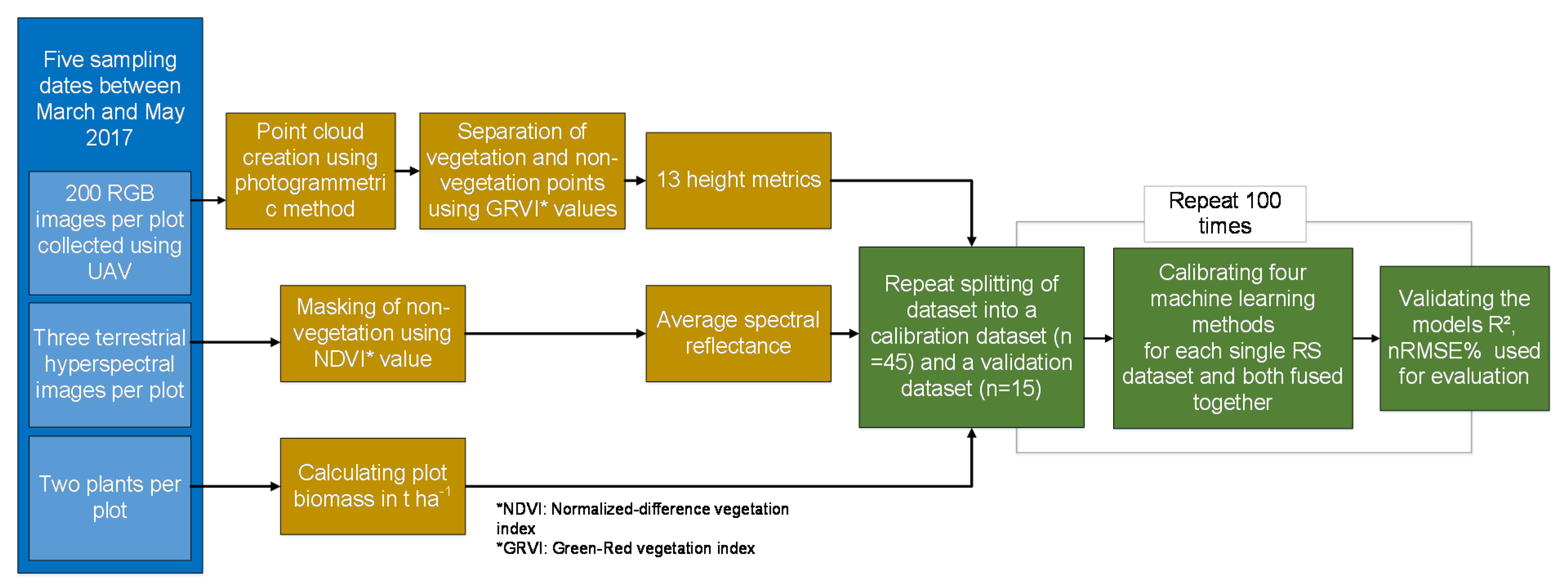
2.5. Statistical Analysis

A two-factorial ANOVA was applied to test for the combined effects of fertilizer and sampling date on the measured biomass. The residuals were checked for normality and homoskedasticity, and base 10 logarithmic transformations were applied as needed to achieve normally distributed residuals.

A wide variety of supervised ML techniques were developed for spatially explicit biomass quantification. Here, four popular ML techniques were used to predict crop biomass for all three crops and to identify the best parameter for prediction (height, spectral, or fusion). ML methods are empirical statistical approaches which can be used to establish statistical relationships between a multitude of explanatory variables (here, spectral bands and height parameters) and response variables (here, crop biomass). ML approaches not only allow the specification of modelling error and quantification of uncertainty [42], but also enable the use of highly correlated explanatory variables. The four selected ML techniques, i.e., partial least squares (PLS), support vector machines (SVM), random forest regression (RFR), and gradient boosting tree (GBT) regression were applied to calibrate the biomass prediction models.

PLS regression searches for a set of latent variables which optimally represent the covariance between the explanatory and response variables. The prediction error of a PLS model decreases with every additional latent variable added to the model until an absolute minimum error is reached. However, this procedure can lead to an overparameterization of the model, resulting in an overoptimistic model. To avoid overparameterization, the search for the optimal number of latent variables was limited to 12, representing 26% of the total number of samples.

SVM regression is a kernel-based statistical approach. The algorithm uses a kernel function to fit the training data to a hyperplane [43]. The radial basis function was used as a kernel. SVM is particularly suitable for fitting complex non-linear data. SVM models can be optimized by tuning several parameters. In the present study, the optimal model was identified using a systematic search for the best cost and sigma parameters [44].

RFR is a tree-based ensemble learning technique combining the information from many independent decision trees to develop the final prediction model [28]. Determination of the optimal tree required optimization of the parameter mtry, defining how many of the total available explanatory variables will be randomly selected at each split in the regression tree. The number of trees per iteration was kept constant at 500 in this study [45]. GBT is another ensemble method, but unlike RFR, each tree is trained based on the results of the previous trees [46].

For model calibration and validation, the dataset for each crop (n = 60) was split up into a calibration dataset (n = 45) and a validation dataset (n = 15) (Figure 2). The optimization procedure for the model calibration of all four ML approaches was done using 10-fold five-times repetition group-leave out cross-validation on the calibration dataset. To accomplish this, 40 samples out of the 45 samples of the calibration dataset were used for the model calibration, while the remaining five samples were used for model optimization (i.e., tuning). This was repeated five times, and the optimal parameters for the calibration model were based on the lowest root–mean–square error (RMSE).

The samples for the remaining validation datasets (n = 15), which were not included in the model calibration, were selected in a stratified random approach. For each sampling date, three samples of the available 12 samples (3 fertilizer treatments × 4 replicates) were randomly chosen and included in the validation dataset.

To find the best combination of ML approach and variables (i.e., spectral, height, or a fusion of both datasets) for predicting the crop biomass, the coefficient of determination using the $R_{val}^2$ (Equation (2)), the prediction error (RMSE_val) (Equation (3)), the relative prediction error (rel.RMSE) (Equation (4)), and the bias (Equation (5)) were calculated as follows

$$R_{val}^2=\left[1-\frac{{{\displaystyle \sum }}_{i=1}^n{\left(y_i-{\widehat{y}}_i\right)}^2}{{{\displaystyle \sum }}_{i=1}^n{\left(y_i-{\overline{y}}_i\right)}^2}\right]$$

(2)

$$RMS{E}_{val}=\sqrt{\frac{{{\displaystyle \sum }}_{i=1}^n{\left({\widehat{y}}_i-y_i\right)}^2}{n}}$$

(3)

$$rel. RMSE = \frac{RMS{E}_{val}}{\max \left(y_i\right)-\min \left(y_i\right)}$$

(4)

$$bias=\frac{1}{n}{{\displaystyle \sum }}_{i=1}^n\left(y_i-{\widehat{y}}_i\right)$$

(5)

where $y_i$ is the measured biomass, ${\widehat{y}}_i$ is the predicted biomass, ${\overline{y}}_i$ is the average measured biomass, and n is the number of samples.

To examine whether the prediction accuracy of crop biomass is different throughout the growing season, an ANOVA was calculated with the deviation between the predicted and measured biomass values as a response variable and sampling date as an explanatory variable.

3. Results

The biomass values for the three crops increased throughout the growing season. For eggplant, the range of all biomass values was from 0.013 to 35.62 t ha⁻¹, while biomass yields were lower for tomato (ranging from 0.015 to 19.04 t ha⁻¹) and higher for cabbage (ranging from 0.026 to 65.66 t ha⁻¹). The biomass values for each crop were log₁₀-transformed for the two-factorial ANOVA in order to achieve normally distributed residuals. The results of the ANOVA (

Table 1. Results of the two-factorial ANOVA testing the effect of sampling date (SD) and fertilizer (NF) on the measured biomass of eggplant, tomato, and cabbage.

	p-Values
	Sampling Date (SD)	N Fertilizer (NF)	SD × NF
Eggplant	***	0.805	0.670
Tomato	***	0.177	0.575
Cabbage	***	0.594	0.972

*** p < 0.001.

) show that there was no significant effect of fertilizer on biomass, which can be explained by the insufficient range of the fertilizer treatments [15]. The effect of sampling date was significant for all three crops, which was expected, as the crops were growing throughout the season. There was no significant interaction between sampling date and fertilizer treatment (Table 1).

Prior to the ML analyses, the intercorrelation between all explanatory variables (i.e., 120 spectral bands and 13 height parameters) was examined. Figure 3 shows a clear intercorrelation between all explanatory variables. However, the pattern of the correlation matrix reveals differences between the three crops. While the wavelengths in the near-infrared spectral region (NIR: 770–950 nm) are highly correlated with the visible bands (VIS: 470–750 nm) for eggplant, this correlation is much weaker for tomato and cabbage. For the 13 height parameters (Table S1), strong correlations (between −0.75 and −1) were found with bands from the VIS spectral range. The height parameters also showed a strong positive correlation among each other.

In total, 3600 ML models were calibrated and validated using the test dataset (Figure 4, Table S2 of the Supplementary Materials). The PLS model using the height dataset or the fused dataset delivered, for all three crops, the most unstable models with $R_{val}^2$ smaller than 0 for 33, 14, six model runs for eggplant, tomato, and cabbage respectively. As these models were particularly worse than all other models, the PLS models using the height dataset were excluded from further analysis. The PLS models using only the spectral dataset were retained in further analysis. The prediction accuracy for the three crops varied strongly depending on the calibration model applied and dataset used (eggplant: $R_{val}^2$ = 0.12–0.99, rel.RMSE = 0.05–0.35, bias = −0.31–0.22; tomato: $R_{val}^2$ = 0.11–0.98, rel.RMSE = 0.05–0.34, bias = −0.28–0.32; cabbage $R_{val}^2$ = 0.50–0.99, rel.RMSE = 0.04–0.25, bias = −0.35–0.19) (Figure 5). For all three crops, RFR showed the best results, with a mean $R_{val}^2$ of 0.96 (range: 0.89–0.99) for eggplant, 0.92 (range: 0.86–0.98) for tomato, and 0.95 (range: 0.86–0.99) for cabbage (Figure 5). The average relative prediction error (rel.RMSE) was largest for tomato (19%), followed by cabbage (13%) and eggplant (12%). For eggplant, the performance of RFR was only slightly better than the best model of the other methods ($R_{val}^2$ = 0.90, 0.93, and 0.96, and rel.RMSE = 12%, 10%, and 11% for PLS, SVR, and GBT, respectively). For tomato, the variation in the mean prediction accuracy among the ML approaches was the largest, with a $R_{val}^2$ of 0.78, 0.75, and 0.72 and a rel.RMSE of 17%, 15%, and 14% for the best-performing models of PLS, SVR, and GBT, respectively (Table S2). For cabbage, the variation in prediction accuracy for the best-performing models was low, with an $R_{val}^2$ of 0.92, 0.91, and 0.88 and a relative error of 10%, 10%, and 11% for PLS, SVR, and GBT, respectively.

In the following, the evaluation of the three sets of variables (spectral, height, and fusion) is described for the best-performing ML models (i.e., RFR) for all crops. The dataset resulting in the most accurate predicted biomass differed between the three crops. For eggplant (Figure 5a, Table S2 Supplementary), the spectral and fusion datasets gave the same prediction accuracy ($R_{val}^2$ = 0.96, rel.RMSE = 0.07, bias = 0.02), indicating that the height parameters did not improve the prediction model based solely on spectral data. For tomato (Figure 5b), the height dataset ($R_{val}^2$ = 0.92, rel.RMSE = 0.09, bias = 0.01) outperformed the spectral dataset alone ($R_{val}^2$ = 0.69, rel.RMSE = 0.20, bias = 0.01) and the fusion of both datasets ($R_{val}^2$ = 0.90, rel.RMSE = 0.11, bias = 0.02) (Table S2). The height dataset was best for predicting cabbage biomass ($R_{val}^2$ = 0.95, rel.RMSE = 0.08, bias = −0.01) (Figure 5c), but did not perform much better than the other two predictor datasets ($R_{val}^2$ = 0.93, rel.RMSE = 0.09, bias = −0.10 for the spectral parameters and $R_{val}^2$ = 0.94, rel.RMSE = 0.9, bias = −0.01 for the fusion dataset).

The effect of sampling date on the deviation between predicted and observed biomass (Figure 6), tested by ANOVA, was not significant. However, for eggplant and tomato (Figure 6a,b), an increasing trend towards underestimation (i.e., deviation < 0) of measured biomass was apparent for the later growth stages (i.e., sampling date 4 and 5).

4. Discussion

The aim of this study was to predict the FMY of three vegetable crops characterized by differing growth forms and internal vegetation structures by means of remote sensing data. Overall, the results show that a high prediction accuracy of FMY can be achieved for all vegetable crops with the chosen methods ($R_{val}^2$ of 0.96 for eggplant, 0.92 for tomato, and 0.95 for cabbage) (Table S2). The presented direct approach (i.e., predicting biomass directly from remotely sensed variables) resulted in much more accurate biomass estimates in comparison to indirect approaches [15,47]. For example, [15] used point cloud-derived height parameters to estimate biomass of the same vegetable crops as in this study via the estimation of the crop height, resulting in a much higher prediction error for all three crops (17.6%, 18.3%, and 15.2% for eggplant, tomato, and cabbage, respectively). While [15] obtained the lowest relative prediction error for cabbage compared to the other crops (rel.RMSE = 15.2%), the lowest relative prediction error in the present study was obtained for eggplant (rel.RMSE = 7.2%). Even for cabbage, the relative prediction error in the present study was much lower (rel.RMSE = 8.3%) (Figure 4). Ref. [48] tested an approach using point-cloud-derived variables and spectral data to predict crop biomass for maize and achieved lower model accuracies than the present study, too. The lower accuracies may be explained by the fact that their spectral information was based on red, green and blue spectral values without the NIR region, which has been shown to be very important for the biomass prediction of vegetation [49].

Regarding the tested ML methods, RFR showed the best prediction performance (based on $R_{val}^2$, rel.RMSE, and bias) for all three crops. RFR frequently outperforms other ML methods in predicting biomass from RS data in agriculture [15,50] and forestry [26,51]. RFR is less sensitive to overfitting than many other methods [52], which might explain the outperformance. Nevertheless, a thorough evaluation of several ML methods should always be conducted, as there is no ML method which consistently outperforms the others under all circumstances (e.g., all ecosystem types and vegetation parameters) [53]. To evaluate the effect of sampling date on FMY prediction, the deviation of the predicted and measured FMY values for each sampling date was estimated (Figure 6). No significant effect of sampling date on the deviation was found, which does not correspond with the results of [54] for maize and sorghum and [15] for eggplant, tomato and cabbage, who both found higher deviations for samples from the early crop stages. [54] argued that a discrepancy in sampling time between the biomass and the RS-based sampling date could be the reason for the larger deviations. Furthermore, high-growing crops like maize or sorghum are characterized by a different growth phenology than vegetable, which makes comparison of the results difficult. In [15], the sampling dates for the biomass harvest and the RS sampling were the same and the author argued that the deviation was most likely driven by inaccuracies during the point cloud processing. Additionally, the heterogenous plant development in the early growth stages of the vegetables might have contributed to the bias in the early growing stages. The slight trend of increasing bias (i.e., biomass underestimation) for the late sampling dates for eggplant and tomato in the present study could be a result of the increased biomass values due to fruit growth, which are no longer related to crop height. A reduced height development, or even a decrease in height at plant maturity, can be found for many crops such as potatoes [55], corn [56], giant ragweed [57], or tomato [58]. Additionally, the reflectance of the entire plant changes throughout the growth [59] due to, e.g., the ripening of fruits and the change in chemical and water content [60], thus changes the relationship between biomass and reflectance [25]. An inclusion of shortwave infrared (>950 nm) spectral information at later growth stages might reduce this bias [61].

For all three crops, the intercorrelation between the explanatory variables (i.e., spectral and height values) was different (Figure 3), particularly in the NIR spectral region, which is known to be strongly related to vegetation biomass and plant internal structure [62]. This could be explained by the different growth forms of the three crops. While eggplant and tomato become tall plants with a dense, closed canopy at the end of the growth period, cabbage is characterized by a rather flat structure and open canopy (i.e., bare ground between the single plants). For tomato, the agricultural practice of tying up the plants with thread might have affected the relationship between biomass and reflectance of NIR. The results of this study, therefore, confirmed the expectation that an individual evaluation of the relationship between biomass and RS variables is necessary for each crop, which has also been shown in, e.g., [15,54,63].

To prove that the fusion of spectral and height information can improve FMY predictions in comparison to single-sensor use, a biomass estimation model based on spectral data and point cloud-derived height information alone and in combination was developed. The sensor data fusion did not result in optimal performance for any of the crops. Although for some of the applied ML approaches, the best model was based on both spectral and height data together (e.g., for the eggplant RFR model, see Table S2), the best model for each crop was always based on a single set of variables, i.e., either spectral or height. This could be partly be explained by the redundancy of the coefficient of determination when using both datasets [22]. [64], which evaluated sensor fusion for crop biomass estimation of maize, found only slight improvements when spectral and lidar data were used together (decrease in prediction error by 0.53 t ha⁻¹), while [65] found a deterioration of prediction accuracy using fused datasets for species identification in shrublands. While for eggplant, the spectral dataset delivered the best prediction accuracies, the model based on the height parameters was best for tomato and cabbage. The tying up of tomato plants from sampling date 3 onwards directly affects the height measurements, and thus the point cloud derivation, which might be an explanation for the selection of the height parameters in the modelling procedure. However, it can be assumed that the biomass and height are still correlated after this agricultural practice until the ripening of the tomato fruits starts. These results confirm the expectation that an evaluation of two or more RS sets of variables reflecting different vegetation characteristics (i.e., spectral reflectance and structure) is as important [65,66] as evaluating different ML methods [50,51].

Overall, the results of the present study proved that estimation of vegetable crop fresh matter biomass using in situ hyperspectral and RGB UAV imagery was successful throughout the growing season. It also clearly demonstrated that optimal models differ among vegetable crops. Although the fusion of both datasets did not outperform single-dataset use, the results indicate that, whenever possible, more than one sensory dataset should be collected to assure an optimal FMY prediction model. However, RGB UAV imagery seems to always be a good choice for receiving good model accuracies, especially when the cost for buying a hyperspectral camera is considered. Furthermore, it was shown that the evaluation of several ML methods using different strategies for building prediction models is worthwhile.

In the future, this approach should be tested using a completely airborne data collection to validate the findings on larger scales and test whether the approach can be used to evaluate the spatial variability of crop biomass under field conditions. This step would allow the further development of precision agriculture in horticultural systems as it would allow to evaluate the phenotypic characteristics of vegetable crops on large scales in a reliable way. The predictive performance of the identified models should be validated with RS data from further growing seasons to check the robustness of the results. Additionally, other sensor systems, such as a thermal imaging system [20], should be tested for their predictive performance for vegetable crop biomass.

References

1. Rockström, J.; Steffen, W.; Noone, K.; Persson, Å.; Chapin, F.S., III; Lambin, E.F.; Lenton, T.M.; Scheffer, M.; Folke, C.; Schellnhuber, H.J.; et al. A safe operating space for humanity. Nature 2009, 461, 472–475. [Google Scholar] [CrossRef] [PubMed]
2. UN. World Population Prospects: The 2017 Revision, Key Findings and Advance Tables; Working Paper No. ESA/P/WP/248; UN: New York, NY, USA, 2017. [Google Scholar]
3. Tilman, D.; Balzer, C.; Hill, J.; Befort, B.L. Global food demand and the sustainable intensification of agriculture. Proc. Natl. Acad. Sci. USA 2011, 108, 20260–20264. [Google Scholar] [CrossRef] [Green Version]
4. Pettorelli, N.; Vik, J.O.; Mysterud, A.; Gaillard, J.-M.; Tucker, C.J.; Stenseth, N.C. Using the satellite-derived NDVI to assess ecological responses to environmental change. Trends Ecol. Evol. 2005, 20, 503–510. [Google Scholar] [CrossRef] [PubMed]
5. Tucker, C.J. Red and photographic infrared linear combinations for monitoring vegetation. Remote Sens. Environ. 1979, 8, 127–150. [Google Scholar] [CrossRef] [Green Version]
6. Atzberger, C. Advances in Remote Sensing of agriculture: Context description, existing operational monitoring systems and major information needs. Remote Sens. 2013, 5, 949–981. [Google Scholar] [CrossRef] [Green Version]
7. Duncan, J.M.A.; Dash, J.; Atkinson, P.M. The potential of satellite-observed crop phenology to enhance yield gap assessments in smallholder landscapes. Front. Environ. Sci. 2015, 3, 132. [Google Scholar] [CrossRef] [Green Version]
8. Hannerz, F.; Lotsch, A. Assessment of remotely sensed and statistical inventories of African agricultural fields. Int. J. Remote Sens. 2008, 29, 3787–3804. [Google Scholar] [CrossRef]
9. Mondal, S.; Jeganathan, C.; Sinha, N.K.; Rajan, H.; Roy, T.; Kumar, P. Extracting seasonal cropping patterns using multi-temporal vegetation indices from IRS LISS-III data in Muzaffarpur District of Bihar, India. Egypt. J. Remote Sens. Space Sci. 2014, 17, 123–134. [Google Scholar] [CrossRef] [Green Version]
10. Thompson, R.B.; Voogt, W.; Incrocci, L.; Fink, M.; de Neve, S. Strategies for optimal fertiliser management of vegetable crops in Europe. Acta Hortic. 2018, 1192, 129–140. [Google Scholar] [CrossRef] [Green Version]
11. Padilla, F.M.; Gallardo, M.; Peña-Fleitas, M.T.; de Souza, R.; Thompson, R.B. Proximal optical sensors for nitrogen management of vegetable crops: A review. Sensors (Basel) 2018, 18, 2083. [Google Scholar] [CrossRef] [Green Version]
12. Trout, T.J.; Johnson, L.F.; Gartung, J. Remote Sensing of Canopy Cover in Horticultural Crops. HortScience 2008, 43, 333–337. [Google Scholar] [CrossRef] [Green Version]
13. Zude-Sasse, M.; Fountas, S.; Gemtos, T.A.; Abu-Khalaf, N. Applications of precision agriculture in horticultural crops. Eur. J. Hortic. Sci. 2016, 81, 78–90. [Google Scholar] [CrossRef]
14. Nidamanuri, R.R.; Zbell, B. Transferring spectral libraries of canopy reflectance for crop classification using hyperspectral Remote Sensing data. Biosyst. Eng. 2011, 110, 231–246. [Google Scholar] [CrossRef]
15. Moeckel, T.; Dayananda, S.; Nidamanuri, R.R.; Nautiyal, S.; Hanumaiah, N.; Buerkert, A.; Wachendorf, M. Estimation of vegetable crop parameter by multi-temporal UAV-borne images. Remote Sens. 2018, 10, 805. [Google Scholar] [CrossRef] [Green Version]
16. Panigrahy, S.; Sharma, S.A. Mapping of crop rotation using multidate Indian Remote Sensing satellite digital data. ISPRS J. Photogramm. Remote Sens. 1997, 52, 85–91. [Google Scholar] [CrossRef]
17. Hoffmeister, D.; Bolten, A.; Curdt, C.; Waldhoff, G.; Bareth, G. (Eds.) High-Resolution Crop Surface Models (CSM) and Crop Volume Models (CVM) on Field Level by Terrestrial Laser Scanning; International Society for Optics and Photonics: Bellingham, WA, USA, 2010. [Google Scholar]
18. Schirrmann, M.; Hamdorf, A.; Giebel, A.; Gleiniger, F.; Pflanz, M.; Dammer, K.-H. Regression Kriging for Improving Crop Height Models Fusing Ultra-Sonic Sensing with UAV Imagery. Remote Sens. 2017, 9, 665. [Google Scholar] [CrossRef] [Green Version]
19. Zhang, C.; Kovacs, J.M. The application of small unmanned aerial systems for precision agriculture: A review. Precis. Agric. 2012, 13, 693–712. [Google Scholar] [CrossRef]
20. Maimaitijiang, M.; Ghulam, A.; Sidike, P.; Hartling, S.; Maimaitiyiming, M.; Peterson, K.; Shavers, E.; Fishman, J.; Peterson, J.; Kadam, S.; et al. Unmanned Aerial System (UAS)-based phenotyping of soybean using multi-sensor data fusion and extreme learning machine. ISPRS J. Photogram. Remote Sens. 2017, 134, 43–58. [Google Scholar] [CrossRef]
21. Aasen, H.; Bolten, A. Multi-temporal high-resolution imaging spectroscopy with hyperspectral 2D imagers—From theory to application. Remote Sens. Environ. 2018, 205, 374–389. [Google Scholar] [CrossRef]
22. Pohl, C.; van Genderen, J.L. Review article multisensor image fusion in Remote Sensing: Concepts, methods and applications. Int. J. Remote Sens. 1998, 19, 823–854. [Google Scholar] [CrossRef] [Green Version]
23. Rischbeck, P.; Elsayed, S.; Mistele, B.; Barmeier, G.; Heil, K.; Schmidhalter, U. Data fusion of spectral, thermal and canopy height parameters for improved yield prediction of drought stressed spring barley. Eur. J. Agron. 2016, 78, 44–59. [Google Scholar] [CrossRef]
24. Gao, S.; Niu, Z.; Huang, N.; Hou, X. Estimating the Leaf Area Index, height and biomass of maize using HJ-1 and RADARSAT-2. Int. J. Appl. Earth Obs. Geoinf. 2013, 24, 1–8. [Google Scholar] [CrossRef]
25. Yue, J.; Feng, H.; Yang, G.; Li, Z. A comparison of regression techniques for estimation of above-ground winter wheat biomass using near-surface spectroscopy. Remote Sens. 2018, 10, 66. [Google Scholar] [CrossRef] [Green Version]
26. Wu, C.; Shen, H.; Shen, A.; Deng, J.; Gan, M.; Zhu, J.; Xu, H.; Wang, K. Comparison of machine-learning methods for above-ground biomass estimation based on Landsat imagery. J. Appl. Remote Sens. 2016, 10, 35010. [Google Scholar] [CrossRef]
27. Wold, S.; Sjöström, M.; Eriksson, L. Partial least squares projections to latent structures (PLS) in chemistry. In Encyclopedia of Computational Chemistry; Ragu Schleyer, P., von Allinger, N.L., Clark, T., Gasteiger, J., Kollman, P.A., Schaefer, H.F., Schreiner, P.R., Eds.; Wiley-Interscience: Hoboken, NJ, USA, 2008; p. 523. ISBN 0470845015. [Google Scholar]
28. Breiman, L. Random Forests. Mach. Learn. 2001, 45, 5–32. [Google Scholar] [CrossRef] [Green Version]
29. Prasad, J.V.N.S.; Rao, C.S.; Srinivas, K.; Jyothi, C.N.; Venkateswarlu, B.; Ramachandrappa, B.K.; Dhanapal, G.N.; Ravichandra, K.; Mishra, P.K. Effect of ten years of reduced tillage and recycling of organic matter on crop yields, soil organic carbon and its fractions in Alfisols of semi arid tropics of southern India. Soil Tillage Res. 2016, 156, 131–139. [Google Scholar] [CrossRef]
30. Harwin, S.; Lucieer, A.; Osborn, J. The impact of the calibration method on the accuracy of point clouds derived using unmanned aerial vehicle multi-view stereopsis. Remote Sens. 2015, 7, 11933–11953. [Google Scholar] [CrossRef] [Green Version]
31. Lowe, D.G. Distinctive image features from scale-invariant keypoints. Int. J. Comput. Vision 2004, 60, 91–110. [Google Scholar] [CrossRef]
32. Snavely, N.; Seitz, S.M.; Szeliski, R. Modeling the world from internet photo collections. Int. J. Comput. Vision 2008, 80, 189–210. [Google Scholar] [CrossRef] [Green Version]
33. Mesas-Carrascosa, F.-J.; Torres-Sánchez, J.; Clavero-Rumbao, I.; García-Ferrer, A.; Peña, J.-M.; Borra-Serrano, I.; López-Granados, F. Assessing optimal flight parameters for generating accurate multispectral orthomosaicks by uav to support site-specific crop management. Remote Sens. 2015, 7, 12793–12814. [Google Scholar] [CrossRef] [Green Version]
34. Westoby, M.J.; Brasington, J.; Glasser, N.F.; Hambrey, M.J.; Reynolds, J.M. ‘Structure-from-Motion’ photogrammetry: A low-cost, effective tool for geoscience applications. Geomorphology 2012, 179, 300–314. [Google Scholar] [CrossRef] [Green Version]
35. Silva, C.A.; Hudak, A.T.; Klauberg, C.; Vierling, L.A.; Gonzalez-Benecke, C.; de Carvalho, S.P.C.; Rodriguez, L.C.E.; Cardil, A. Combined effect of pulse density and grid cell size on predicting and mapping aboveground carbon in fast-growing Eucalyptus forest plantation using airborne LiDAR data. Carbon Balance Manag. 2017, 12, 13. [Google Scholar] [CrossRef] [PubMed] [Green Version]
36. Næsset, E.; Økland, T. Estimating tree height and tree crown properties using airborne scanning laser in a boreal nature reserve. Remote Sens. Environ. 2002, 79, 105–115. [Google Scholar] [CrossRef]
37. Roussel, J.-R.; Auty, D. lidR: Airborne LiDAR data manipulation and visualization for forestry applications. R Package Version 2018, 1, 1. Available online: https://CRAN.R-project.org/package=lidR (accessed on 10 October 2020).
38. R Core Team. R: A Language and Environment for Statistical Computing; R Core Team: Vienna, Austria, 2018; Available online: https://www.R-project.org/ (accessed on 10 October 2020).
39. Cao, F.; Yang, Z.; Ren, J.; Jiang, M.; Ling, W.-K. Does Normalization Methods Play a Role for Hyperspectral Image Classification? arXiv 2017, arXiv:1710.02939. [Google Scholar]
40. Mosin, V.; Aguilar, R.; Platonov, A.; Vasiliev, A.; Kedrov, A.; Ivanov, A. Remote Sensing and machine learning for tree detection and classification in forestry applications. In Proceedings of the Image and Signal Processing for Remote Sensing XXV, Strasbourg, France, 9–12 September 2019; Bruzzone, L., Bovolo, F., Benediktsson, J.A., Eds.; SPIE: Bellingham, WA, USA, 2019; p. 14, ISBN 9781510630130. [Google Scholar]
41. Rouse, J.W., Jr.; Haas, R.H.; Schell, J.A.; Deering, D.W. Monitoring vegetation systems in the Great Plains with ERTS. NASA Spec. Publ. 1974, 351, 309. [Google Scholar]
42. Holloway, J.; Mengersen, K. Statistical machine learning methods and Remote Sensing for sustainable development goals: A Review. Remote Sens. 2018, 10, 1365. [Google Scholar] [CrossRef] [Green Version]
43. Cortes, C.; Vapnik, V. Support-vector networks. Mach. Learn. 1995, 20, 273–297. [Google Scholar] [CrossRef]
44. Karatzoglou, A.; Meyer, D.; Hornik, K. Support vector machines in R. J. Stat. Softw. 2006, 15, 1–28. [Google Scholar] [CrossRef] [Green Version]
45. Probst, P.; Boulesteix, A.-L. To Tune or Not to Tune the Number of Trees in Random Forest. J. Mach. Learn. Res. 2018, 18, 1–18. [Google Scholar]
46. Caruana, R.; Niculescu-Mizil, A. An empirical comparison of supervised learning algorithms using different performance metrics. In Proceedings of the 23rd International Conference on Machine Learning, Pittsburgh, WA, USA, 25–29 June 2006; pp. 161–168. [Google Scholar]
47. Madec, S.; Baret, F.; de Solan, B.; Thomas, S.; Dutartre, D.; Jezequel, S.; Hemmerlé, M.; Colombeau, G.; Comar, A. High-throughput phenotyping of plant height: Comparing unmanned aerial vehicles and ground LiDAR estimates. Front. Plant Sci. 2017, 8, 2002. [Google Scholar] [CrossRef] [Green Version]
48. Li, W.; Niu, Z.; Chen, H.; Li, D.; Wu, M.; Zhao, W. Remote estimation of canopy height and aboveground biomass of maize using high-resolution stereo images from a low-cost unmanned aerial vehicle system. Ecol. Indic. 2016, 67, 637–648. [Google Scholar] [CrossRef]
49. Bendig, J.; Yu, K.; Aasen, H.; Bolten, A.; Bennertz, S.; Broscheit, J.; Gnyp, M.L.; Bareth, G. Combining UAV-based plant height from crop surface models, visible, and near infrared vegetation indices for biomass monitoring in barley. Int. J. Appl. Earth Observ. Geoinf. 2015, 39, 79–87. [Google Scholar] [CrossRef]
50. Nasi, R.; Viljanen, N.; Kaivosoja, J.; Alhonoja, K.; Hakala, T.; Markelin, L.; Honkavaara, E. Estimating biomass and nitrogen amount of barley and grass using UAV and aircraft based spectral and photogrammetric 3D features. Remote Sens. 2018, 10, 1082. [Google Scholar] [CrossRef] [Green Version]
51. Powell, S.L.; Cohen, W.B.; Healey, S.P.; Kennedy, R.E.; Moisen, G.G.; Pierce, K.B.; Ohmann, J.L. Quantification of live aboveground forest biomass dynamics with Landsat time-series and field inventory data: A comparison of empirical modeling approaches. Remote Sens. Environ. 2010, 114, 1053–1068. [Google Scholar] [CrossRef]
52. Belgiu, M.; Drăguţ, L. Random forest in Remote Sensing: A review of applications and future directions. ISPRS J. Photogram. Remote Sens. 2016, 114, 24–31. [Google Scholar] [CrossRef]
53. Flach, P. Machine learning. The Art and Science of Algorithms that Make Sense of Data; Cambridge University Press: Cambridge, UK, 2012; ISBN 9781107422223. [Google Scholar]
54. Malambo, L.; Popescu, S.C.; Murray, S.C.; Putman, E.; Pugh, N.A.; Horne, D.W.; Richardson, G.; Sheridan, R.; Rooney, W.L.; Avant, R.; et al. Multitemporal field-based plant height estimation using 3D point clouds generated from small unmanned aerial systems high-resolution imagery. Int. J. Appl. Earth Observ. Geoinf. 2018, 64, 31–42. [Google Scholar] [CrossRef]
55. Schulz, V.S.; Munz, S.; Stolzenburg, K.; Hartung, J.; Weisenburger, S.; Graeff-Hönninger, S. Impact of Different Shading Levels on Growth, Yield and Quality of Potato (Solanum tuberosum L.). Agronomy 2019, 9, 330. [Google Scholar] [CrossRef] [Green Version]
56. Çakir, R. Effect of water stress at different development stages on vegetative and reproductive growth of corn. Field Crops Res. 2004, 89, 1–16. [Google Scholar] [CrossRef]
57. Kaur, S.; Aulakh, J.; Jhala, A.J. Growth and seed production of glyphosate-resistant giant ragweed (Ambrosia trifida L.) in response to water stress. cjps 2016, 96, 828–836. [Google Scholar] [CrossRef] [Green Version]
58. Paradiso, R.; Arena, C.; de Micco, V.; Giordano, M.; Aronne, G.; de Pascale, S. Changes in Leaf Anatomical Traits Enhanced Photosynthetic Activity of Soybean Grown in Hydroponics with Plant Growth-Promoting Microorganisms. Front. Plant Sci. 2017, 8, 674. [Google Scholar] [CrossRef] [Green Version]
59. Viña, A.; Gitelson, A.A.; Rundquist, D.C.; Keydan, G.; Leavitt, B.; Schepers, J. Monitoring Maize (L.) Phenology with Remote Sensing. Agron. J. 2004, 96, 1139. [Google Scholar] [CrossRef]
60. Kurunç, A.; Ünlükara, A. Growth, yield, and water use of okra (Abelmoschus esculentus ) and eggplant (Solanum melongena ) as influenced by rooting volume. New Zeal. J. Crop Hort. Sci. 2009, 37, 201–210. [Google Scholar] [CrossRef]
61. Rasooli Sharabian, V.; Noguchi, N.; Ishi, K. Optimal vegetation indices for winter wheat growth status based on multi-spectral reflectance. Environ. Control. Biol. 2013, 51, 105–112. [Google Scholar] [CrossRef]
62. Knipling, E.B. Physical and physiological basis for the reflectance of visible and near-infrared radiation from vegetation. Remote Sens. Environ. 1970, 1, 155–159. [Google Scholar] [CrossRef]
63. Viña, A.; Gitelson, A.A.; Nguy-Robertson, A.L.; Peng, Y. Comparison of different vegetation indices for the remote assessment of green leaf area index of crops. Remote Sens. Environ. 2011, 115, 3468–3478. [Google Scholar] [CrossRef]
64. Wang, C.; Nie, S.; Xi, X.; Luo, S.; Sun, X. Estimating the biomass of maize with hyperspectral and LiDAR data. Remote Sens. 2017, 9, 11. [Google Scholar] [CrossRef] [Green Version]
65. Prošek, J.; Šímová, P. UAV for mapping shrubland vegetation: Does fusion of spectral and vertical information derived from a single sensor increase the classification accuracy? Int. J. Appl. Earth Observ. Geoinf. 2019, 75, 151–162. [Google Scholar] [CrossRef]
66. Tilly, N.; Hoffmeister, D.; Cao, Q.; Huang, S.; Lenz-Wiedemann, V.; Miao, Y.; Bareth, G. Multitemporal crop surface models: Accurate plant height measurement and biomass estimation with terrestrial laser scanning in paddy rice. J. Appl. Remote Sens. 2014, 8, 083671. [Google Scholar] [CrossRef]
Figure 1. (a) Position of Bengaluru within India. (b) Design of the experimental layout used in this study. Different grey levels indicate the three investigated crops (white: cabbage, light grey: eggplant, and dark grey: tomato: The pattern indicates the level of nitrogen fertilization (no pattern: low, dotted: medium, and squares: high fertilization). H and S indicate the sampling plots for the destructive biomass samples (S) and the sensor data collection (H). (adjusted from [15]).
Agronomy 10 01600 g001
Figure 2. Workflow describing the data collection (blue), data preparation (yellow), and data analysis scheme (green).
Agronomy 10 01600 g002
Figure 3. Intercorrelation between all explanatory variables (i.e., 120 spectral bands and 13 height parameters) for (a) eggplant, (b) tomato, and (c) cabbage.
Agronomy 10 01600 g003
Figure 4. Results from cross-validation using three sets of variables (left: height, middle: spectral, and right: fusion) and machine learning approaches (Random Forest (RFR), Partial Least Squares (PLS), Support Vector (SVR), and Gradient Boosting Tree (GBT)). The distribution of the normalized prediction error (rel.RMSE) the coefficient of determination ( R v a l 2 ) and the bias is shown as a violin plot (Potter et al., 2006) for (a) eggplant, (b) tomato, and (c) cabbage. The areas around the lines indicate the probability density of the data.
Agronomy 10 01600 g004
Figure 5. Predicted versus observed biomass based on the best machine learning method (i.e., random forest regression) for 100 validation datasets based on the best performing explanatory set of variables for (a) eggplant, predicted using the spectral variables, (b) tomato, predicted using the height parameters, and (c) cabbage, predicted using the height variables. The prediction quality measures (i.e., R v a l 2 and r e l . R M S E v a l ) are averaged over all 100 model runs. The blue line indicates the linear relationship of the values while the dotted line shows the 1:1 (perfect fit) line.
Agronomy 10 01600 g005
Figure 6. Normalized deviations of the predicted from the observed values for (a) eggplant, (b) tomato, and (c) cabbage for each sampling date. The dotted line indicates zero deviation and thus perfect fit between measured and predicted biomass values. The areas around the lines indicate the probability density of the data.
Agronomy 10 01600 g006