An Arable Field for Benchmarking of Metaheuristic Algorithms for Capacitated Coverage Path Planning Problems

Abstract

This study specifies an agricultural field (Latitude = 56°30′0.8″ N, Longitude = 9°35′27.88″ E) and provides the absolute optimal route for covering that field. The calculated absolute optimal solution for this field can be used as the basis for benchmarking of metaheuristic algorithms used for finding the most efficient route in the field. The problem of finding the most efficient route that covers a field can be formulated as a Traveling Salesman Problem (TSP), which is an NP-hard problem. This means that the optimal solution is infeasible to calculate, except for very small fields. Therefore, a range of metaheuristic methods has been developed that provide a near-optimal solution to a TSP in a “reasonable” time. The main challenge with metaheuristic methods is that the quality of the solutions can normally not be compared to the absolute optimal solution since this “ground truth” value is unknown. Even though the selected benchmarking field requires only eight tracks, the solution space consists of more than 1.3 billion solutions. In this study, the absolute optimal solution for the capacitated coverage path planning problem was determined by calculating the non-working distance of the entire solution space and determining the solution with the shortest non-working distance. This was done for four scenarios consisting of low/high bin capacity and short/long distance between field and storage depot. For each scenario, the absolute optimal solution and its associated cost value (minimum non-working distance) were compared to the solutions of two metaheuristic algorithms; Simulated Annealing Algorithm (SAA) and Ant Colony Optimization (ACO). The benchmarking showed that neither algorithm could find the optimal solution for all scenarios, but they found near-optimal solutions, with only up to 6 pct increasing non-working distance. SAA performed better than ACO, concerning quality, stability, and execution time.

1. Introduction

In recent years, much research effort has targeted solutions to Coverage Path Planning (CPP) problems in arable farming. When multiple points of interest are to be visited, coverage path planning can be formulated as a Traveling Salesman Problem (TSP) [1], or more generally a Vehicle Routing Problem (VRP) [2]. As known, these classes of optimization problems are non-deterministic polynomial-time hard (NP-hard). CPP is a variant of TSP where, instead of visiting each point of interest, an agent must visit all paths between these points. The objective is to minimize the total travel length of the agent [3,4]. The computational time required to solve the problem increases extremely when the dimension of the problem, i.e., the number of paths to visit, increases.

In the Vehicle Routing Problem (VRP), a single capacitated vehicle is responsible for delivering items to multiple customer nodes; the vehicle must return to the depot to pick up additional items when it is emptied. The optimal route depends on the storage capacity of the vehicle. Many agricultural field operations can be cast as a VRP/CPP problem, for example, seeding and fertilization; a capacitated machine must cover the entire field and distribute material from a depot to the field. When the storage tank on the machine is empty, the machine must return to the depot for refilling. Harvest is similar, except that the direction of material flow is opposite, from the field to the depot [5]. To formulate a field operation as a VRP, the field is divided into tracks that cover the field. The endpoints of tracks are represented as nodes in a network graph, together with the depot. The costs of traveling between any nodes are represented in a cost matrix. The optimization problem consists of finding the route through all tracks with the lowest total cost, subject to the constraints given by the capacity of the machine and the material demands of the tracks [6].

This problem is computationally difficult to solve in terms of obtaining optimality for fields of a realistic size and has led to many researchers investigating the efficiency and focusing on improving algorithms for various path generation methods [7,8,9]. For instance, [10] investigated the CPP problem in capacitated field operations and compared the calculated plans to real fertilizing applications. As mentioned, VRP and CRP are NP-hard, so finding an absolute shortest path is difficult in low dimensions and is impossible in high dimensions. Although, computer scientists have paid considerable attention to the VRP, solving the problem by spending a lot of time by an exact algorithm [11]. As an alternative to searching the entire search space for the global optimum solution (also called the absolute solution), metaheuristic search algorithms have been developed with the ambition to find near-optimal solutions in a realistic time [12]. Over the years, a branch-and-bound algorithm and a branch-and-cut algorithm developed different solution approaches [13,14,15], heuristic algorithms (such as the Clarke–Wright savings algorithm [16]), and metaheuristic algorithms (such as simulated annealing [17,18], genetic algorithms [19], tabu search [20], and ant algorithms [21].

There is a need for benchmarking optimization algorithms against each other for efficiency and quality. There are many benchmarking functions and datasets which are used for testing and evaluating the optimization algorithms [22,23,24,25]. In the lack of a common benchmarking standard, researchers have applied different agricultural fields to show the performance of their algorithm [7,10,26,27,28]. Obviously, algorithms can only be compared if they have been tested under similar conditions, notably on a common benchmarking field. This is necessary in order to compare the efficiency and performance of metaheuristic algorithms in CPP under similar boundary conditions. Currently, such a benchmarking field for comparison of the efficiency and performance of metaheuristic algorithms in CPP, where the global optimum is known, has not yet been described in the literature, to the best of our knowledge.

In this paper, a field has been selected and described as a qualified candidate for a common benchmarking field for existing and future optimization algorithms. Due to the small size of this field (eight tracks), it is possible to determine the entire search space (1.3 billion potential solutions to the CPP problem) and to find the absolute optimal solution with the lowest cost. The absolute optimal solution has been calculated for each of four scenarios, as a combination of two values of bin capacity and two values of distance between field and depot. The chosen field was used to benchmark two metaheuristic algorithms, Simulated Annealing Algorithm (SAA) and Ant Colony Optimization (ACO). The solutions of these metaheuristic algorithms were compared with the absolute optimal solution.

2. Materials and Methods

In this section, the selected agricultural field for benchmark of metaheuristic algorithms was adopted to determine all the possible capacitated coverage solutions of the field and to find the absolute optimal solution, which is a coverage plan for the field with minimum non-working driving distance concerning the constraints of the capacitated field operation. The two metaheuristic algorithms, simulated annealing algorithm (SAA) and ant colony optimization (ACO), were examined and their near-optimal solutions were compared to the absolute solution for the candidate field. When selecting the benchmarking field, the complexity of the problem should be taken into account since the size of the solution space depends on the number of tracks in the field.

2.1. Terminology

Most field operations require that the field is covered exactly once; ideally, no part of the field should receive neither none nor multiple treatments. To achieve this, it is convenient to represent the field geometrically. This is done by selecting a driving direction and dividing the field area into parallel rows along the driving direction with a width equal to the working width of the machine used for the operation in question. The centerline of each row is called a track and by following the track of each row the field will be covered. In order to change from one track to another, an area for turning is defined at the end of the rows. This area is denoted the headland, and the remaining part of the field is denoted the field body. In some operations, notably harvesting, the headland is treated before the field body to make room for the turnings; however, in operations such as fertilization, the headland is normally treated after the field body. The width of the headland must be sufficient for the machine to turn, and additionally, it must be an integral multiple of the working width. This number is called the headland pass. The total distance driven to cover the field can be divided into the working distance and the non-working distance. The working distance is constant and can be calculated as the field area in square meters divided by the working width in meters. The non-working distance, which is the optimization criterion in this work, is the total unproductive distance, e.g., for changing tracks. For capacitated field operations, material is either removed from (harvest) or brought into (sowing, fertilization, etc.) the field. The material is collected from or delivered to a depot. The material is transported in a bin with a certain bin capacity. In this study, we require the bin capacity to be sufficient to cover the demand of any track. We also only consider a single depot for simplicity.

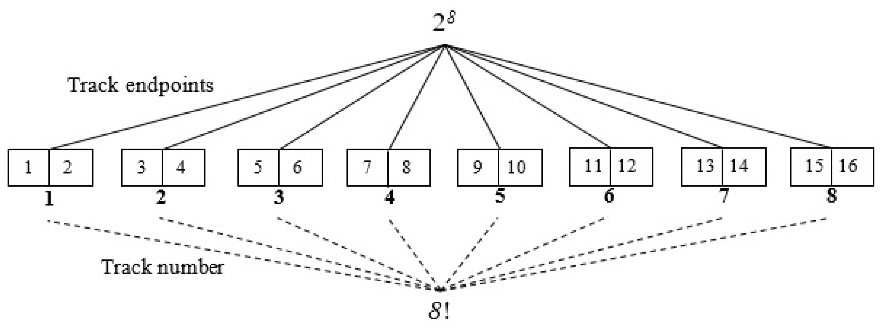
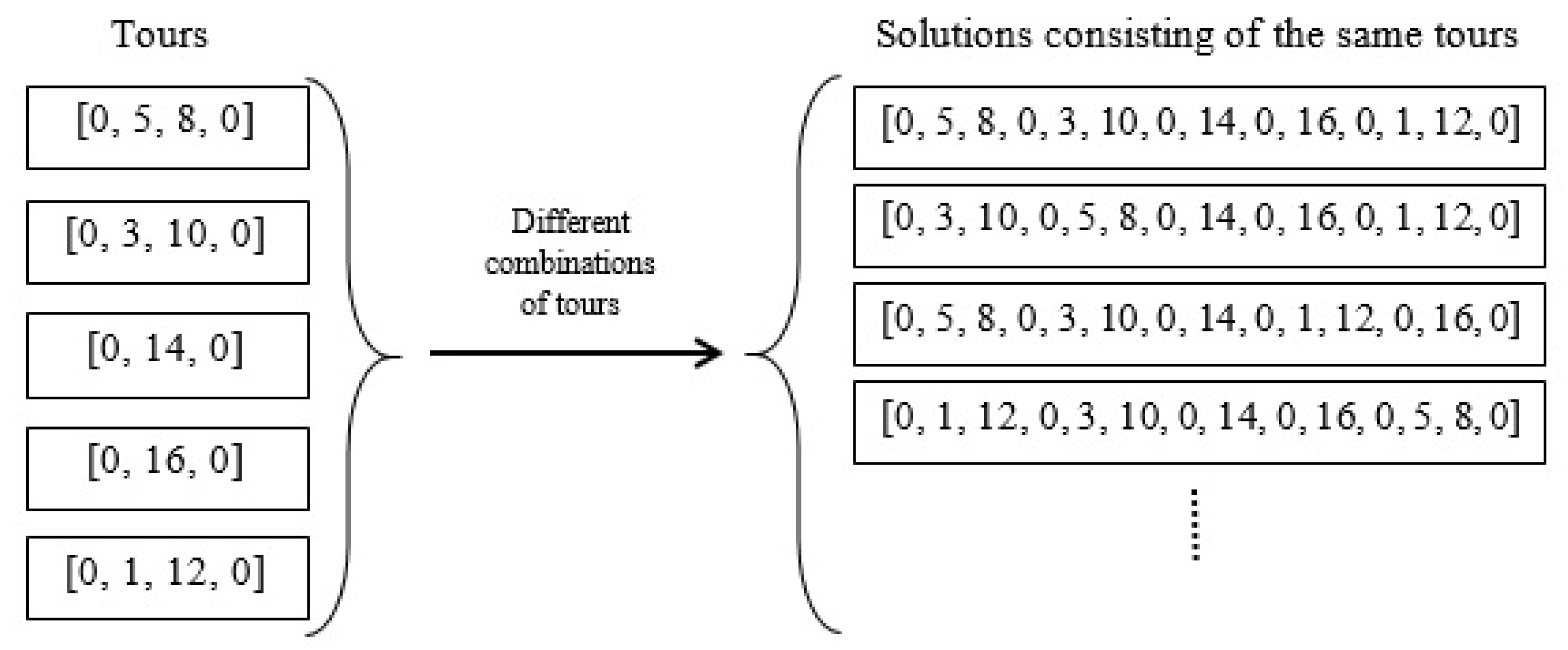
Any ordering of the tracks of a field with a direction of the tracks constitutes a route or a solution to the covering problem. The cost of a solution is the total non-working distance of the coverage. An optimal or an absolute solution is a solution with the lowest cost value. Since the cost value is dependent on both the order and the driving direction of the tracks, it can be listed by the sequence of endpoints of the tracks. If a field has N tracks, the endpoints of the ith track can be noted 2i − 1 and 2i, for i = 1, …, N. A track can be referred to either by its number, i, or by its endpoints, [2i − 1, 2i]. For a field with 8 tracks, a solution could be noted as a sequence of all 16 track endpoints, e.g., [0, 8, 7, 11, 12, 6, 5, 1, 2, 4, 3, 9, 10, 16, 15, 13, 14, 0], where 0 is a common starting and ending point of the route. In this solution, the first track to visit is number 4 in the direction from endpoint 8 to 7, then track 6 in the direction from endpoint 11 to 12, and so forth. The same solution can be written simpler by only listing the entry endpoints of the tracks: [0, 8, 11, 6, 1, 4, 9, 16, 13, 0] since the exit endpoint is given from the entry. For a capacitated operation, 0 indicates the ID of the depot and the solution includes 0’s when the machine must return to the depot to refill/unload, e.g., [0, 8, 11, 6, 1, 0, 4, 9, 16, 13, 0]. This solution contains a single refill/unload visit to the depot, so it consists of two tours, i.e., [0, 8, 11, 6, 1, 0] and [0, 4, 9, 16, 13, 0]. Two tours are considered equivalent if they consist of the same tracks, only in opposite direction. Moreover, two solutions are equivalent if they consist of the same or equivalent tours in different orderings.

2.2. Calculating the Number of Solutions

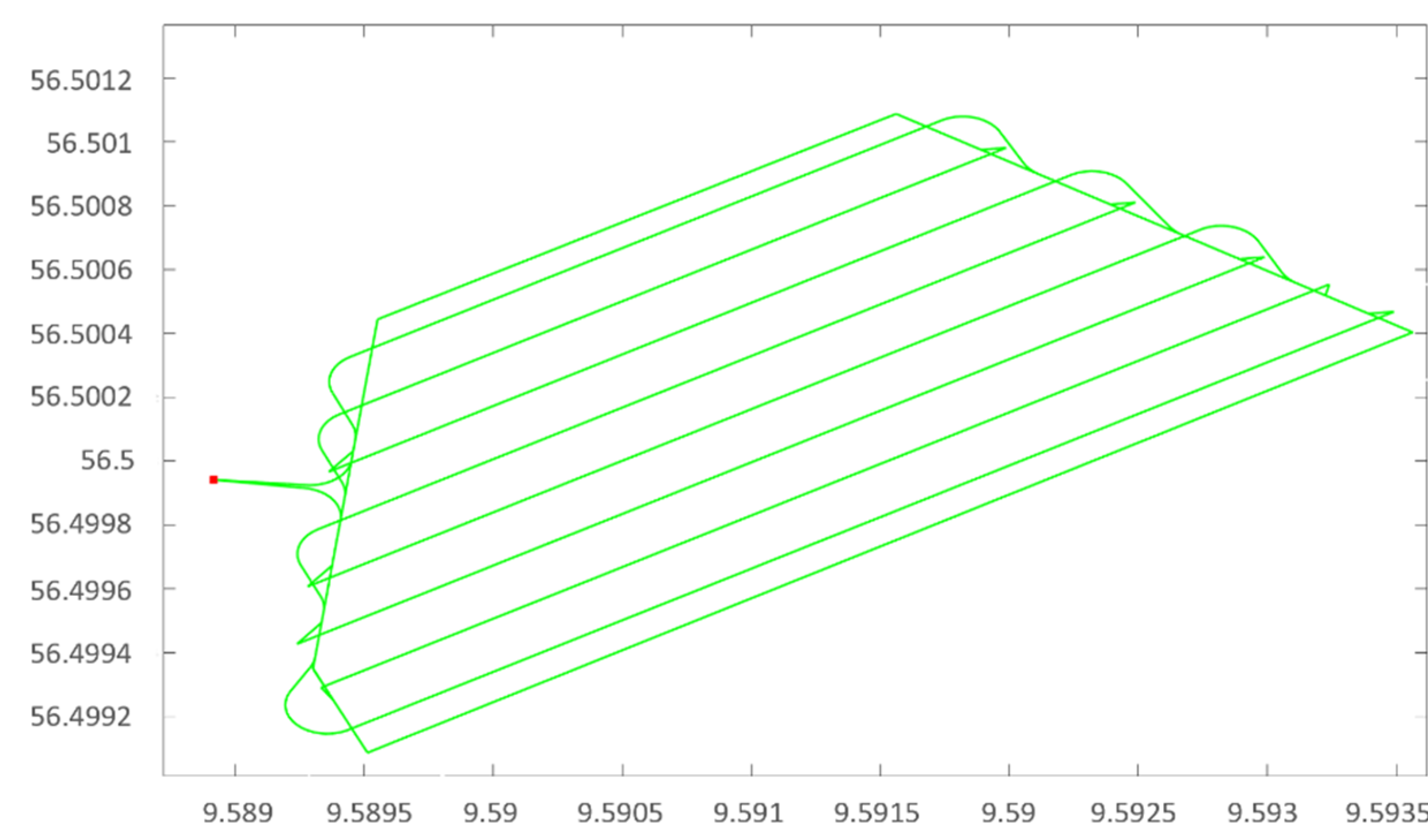
The size of the solution space has been calculated as a function of the number of tracks, N. Figure 1 illustrates the number of different ways to cover a field with N = 8 tracks when an uncapacitated operation is considered, and each track must be visited exactly once. The 8 tracks can be permuted in 8! ways and each track can be traversed in one of two directions $\left(\uparrow \downarrow \right)$. This results in $2^8·8! =$ = 10,321,920. different solutions which is demonstrated in the Figure 1. In general, the number of solutions P_N for an uncapacitated operation in a field with N tracks is expressed by (1):

$${\mathcal{P}}_N=2^N·N!$$

(1)

Considering one of the P₈ possible solutions, say [0, 8, 11, 6, 1, 4, 9, 16, 13, 0], it can be changed into a solution for a capacitated operation by adding zeroes, corresponding to visits at the depot for unloading/refilling the bin. For example [0, 8, 11, 0, 6, 1, 4, 9, 0, 16, 13, 0] is a solution with two intermediate depot visits. The number of ways to add two zeroes between the eight-track endpoints is equal to the number of ways 2 items can be selected from 7, namely 21 which is shown in (2):

$$C\left(7,2\right)=\frac{7!}{2!\left(7-2\right)!}=21$$

(2)

Thus, in general, the number of capacitated solutions corresponding to each uncapacitated is calculated as the number of ways to add 0, 1, 2,…, N − 1 zeroes between the N track endpoints. This is expressed in (3):

$${\mathcal{C}}_N=C\left(N-1,0\right)+C\left(N-1,1\right)+\cdots +C\left(N-1,N-1\right)={\displaystyle \sum }_{i=0}^{N-1}\frac{\left(N-1\right)!}{i!\left(N-i-1\right)!}=2^{N-1}$$

(3)

Finally, the total number of solutions to cover a field with N tracks with a capacitated operation is shown in (4):

$${\mathcal{T}}_N={\mathcal{P}}_N{\mathcal{C}}_N=2^N·N!·2^{N-1}=N!·2^{\left(2N-1\right)}$$

(4)

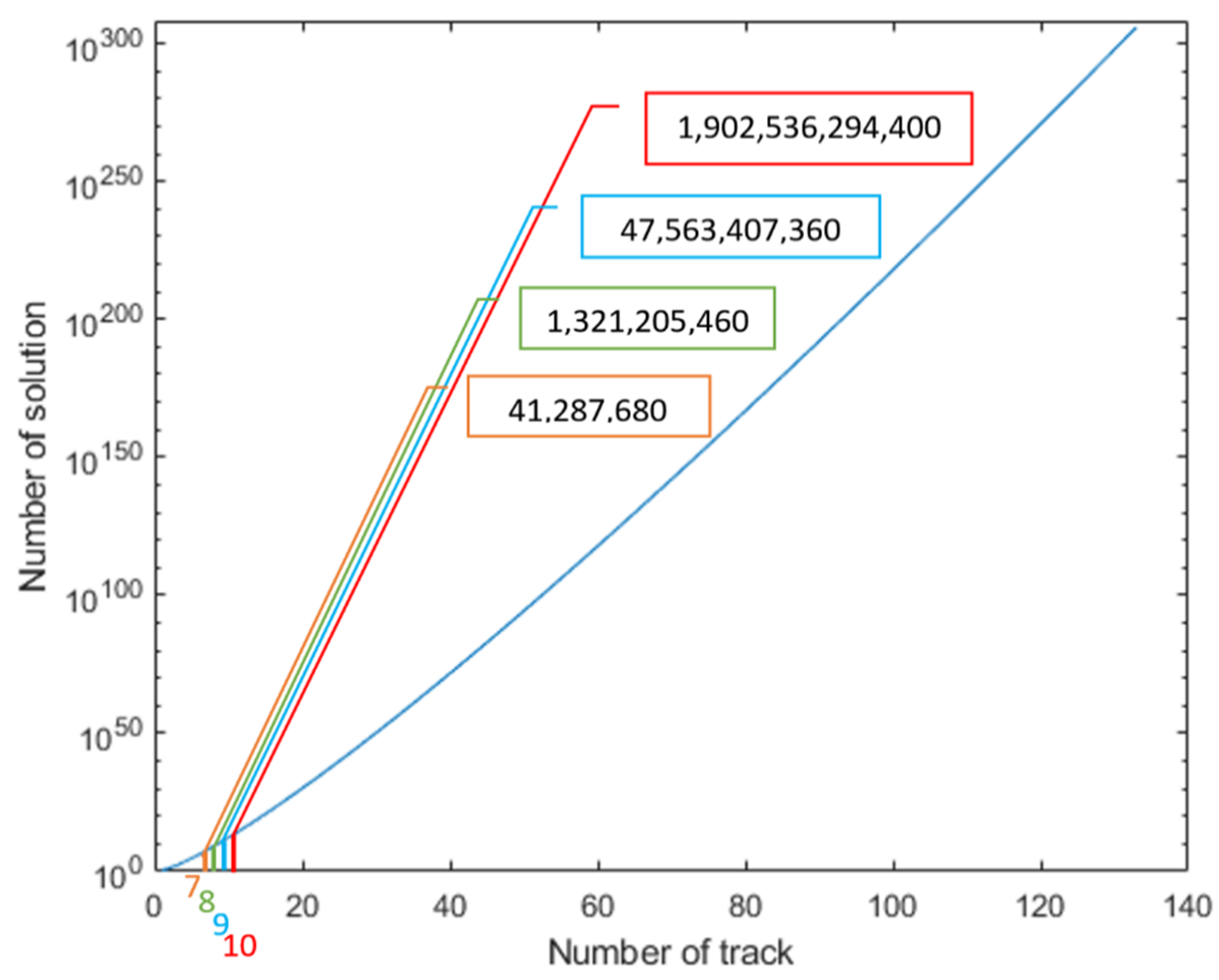
The total number of solutions for seven, eight, nine, and ten tracks are shown in

Table 1. Number of solutions for uncapacitated (${\mathcal{P}}_N$) and capacitated (${\mathcal{T}}_N$) operations in a field with N tracks.

$\mathit{N}$	${\mathcal{P}}_{\mathit{N}}$	${\mathcal{C}}_{\mathit{N}}$	${\mathcal{T}}_{\mathit{N}}$
7	645,120	64	41,287,680
8	10,321,920	128	1,321,205,760
9	185,794,560	256	47,563,407,360
10	3,715,891,200	512	1,902,536,294,400

.

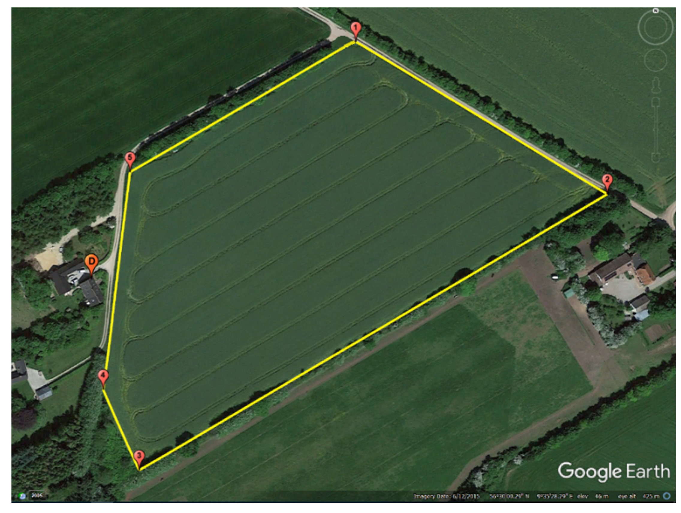
Figure 2 shows how the number of solutions, T_N, increases dramatically with the increasing number of tracks, N. The logarithmic scale reveals that the solution size increases even faster than exponentially. Based on these calculations it was decided to select a benchmarking field with eight tracks to make it feasible to create and evaluate all possible solutions and determine the optimal solution for comparison by metaheuristic algorithms.

2.3. Selecting the Benchmarking Field

The field for benchmarking of optimization algorithms was selected as a relatively small field (2.97 hectares) with eight tracks. The field is located in Denmark (Lat. = 56°30′0.89″ N, Lon. = 9°35′27.88″ E) and is shown in Figure 3. The field border forms an irregular, convex polygon with five corner points. A polygon is convex if all interior angles are less than 180 degrees, otherwise, it is concave. All eight tracks have different lengths, which makes it convenient for benchmarking of CPP algorithms.

Table 2. Coordinates of depot and field polygon corners.

Name of Point	Latitude	Longitude
Depot (D)	56°29′59.7840″ N	9°35′20.1032″ E
Point (1)	56°30′04.5012″ N	9°35′29.6780″ E
Point (2)	56°30′01.4380″ N	9°35′38.6329″ E
Point (3)	56°29′55.9689″ N	9°35′21.8232″ E
Point (4)	56°29′57.5760″ N	9°35′20.5319″ E
Point (5)	56°30′01.9144″ N	9°35′21.5229″ E

shows he coordinates of the depot and the six corner points of the field polygon.

2.4. Calculating All Possible Solutions and Determining the Best

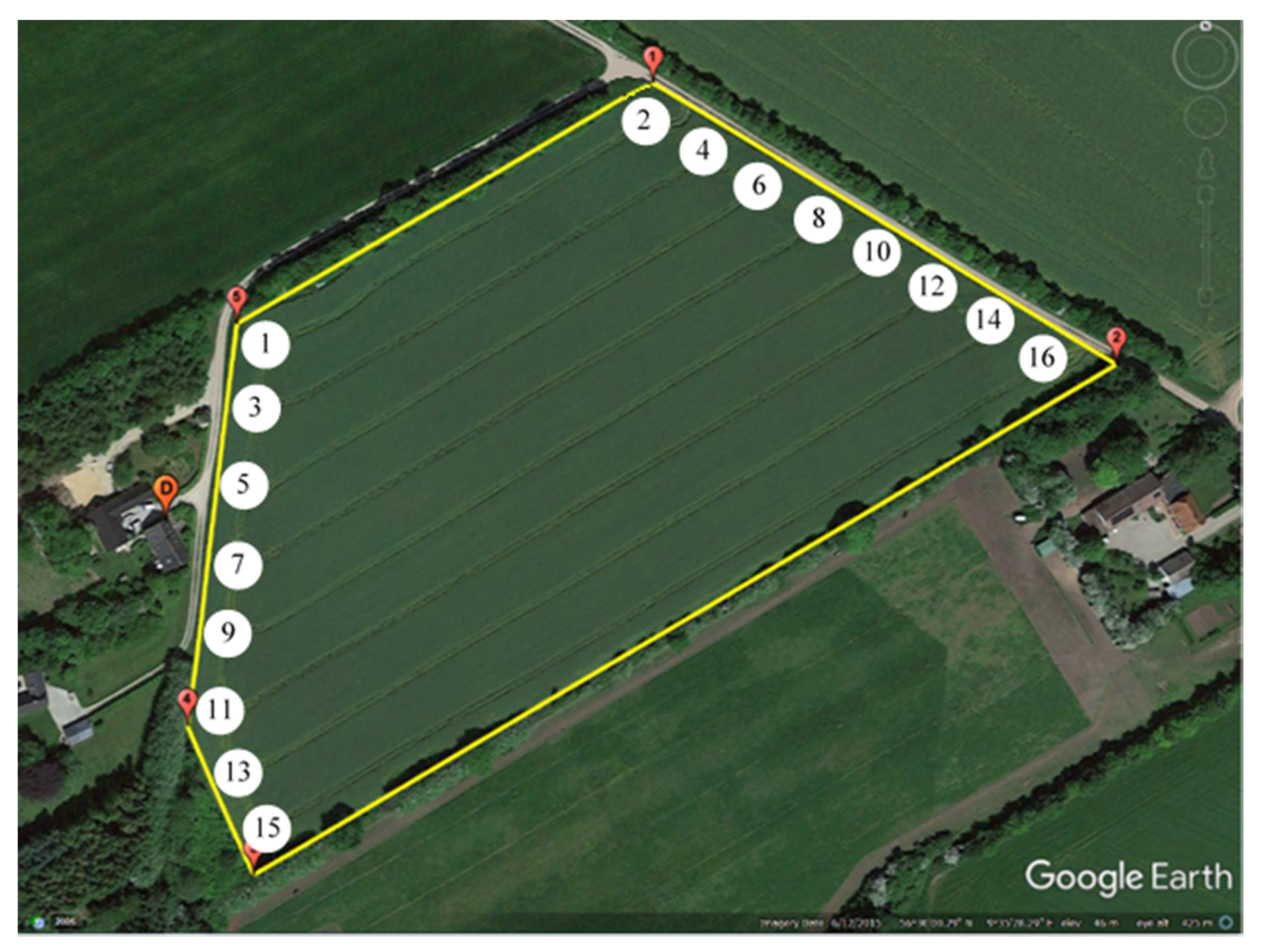
In order to calculate the non-working distance of all 1,321,205,760 solutions of the benchmarking field (Figure 3) a geometrical representation of the field was made according to the method introduced by [29]. Slurry fertilization was selected as a representative capacitated operation, and necessary input variables to specify the field, operation, machine, and implement were assigned values, as shown in

Table 3. Input variables and selected values.

Name of Variable	Value of Variable (Unit)
Working width of fertilizer	16 (meter)
Number of headland passes	1
Minimum turning radius of implement	10 (meter)
Fertilizer requirement of field	43,000 (liter/hectare)
Bin capacity	30,000 and 46,000 (liter)
Driving Direction	Point (2) and Point (3)

.

Based on the method presented in [10,26,29] a geometrical representation of the field was produced, as shown in Figure 4. This included a representation of the field polygon, tracks with coordinates of their endpoints, turnings between tracks, coordinates of the depot, as well as the length and demand of each track. The demand for a track was calculated proportionally to its length, such that the fertilizer requirement was distributed evenly over the area.

The tracks were numbered and given endpoint IDs as shown in Figure 5. The resulting track lengths and demands are shown in

Table 4. Lengths and fertilizer demand of the tracks.

Track Number	Track 1	Track 2	Track 3	Track 4	Track 5	Track 6	Track 7	Track 8
Endpoints	[1, 2]	[3, 4]	[5, 6]	[7, 8]	[9, 10]	[11, 12]	[13, 14]	[15, 16]
Length (m)	163.34	184.11	204.88	225.66	246.43	267.21	278.41	288.68
Demand (L)	11,237	12,667	14,096	15,525	16,955	18,384	19,154	19,861

.

It is important to note that not all ${\mathcal{T}}_8$ = 1,321,205,760 solutions are feasible. A solution is not feasible if it contains a tour where the sum of demands of the tracks of the tour, according to the track demands of Table 4, exceeds the bin capacity displayed in Table 3.

Graph modelling was applied to generate a field graph consist of all the types of edges (connections) in the field. There are six types of edges between each pair of the vertices and each defined edge has a length [18]:

• Gate to Headland (G2H): two edges connect the gate to the headland path
• Headland (H): the connection between two subsequent vertices in headland path
• Track (T): the connection between two pairs of nodes (two ends of a fieldwork area).
• Track to Headland (T2H): the connection between track nodes and vertices in the headland
• Track to track (T2T): the connection between the end nodes of two adjacent tracks
• Headland to headland (H2H): the connection between two headland paths

These turns are generated based on the Dubin’s Curves method [30]. In graph search, to find the shortest non-working distance between each pair of endpoints, Dijkstra’s method is applied [31]. This resulted in the cost matrix (

Table A1. Cost matrix of the benchmarking field.

Node’s Id	0	1	2	3	4	5	6	7	8	9	10	11	12	13	14	15	16
0	0.00	77.53	241.77	70.52	260.22	50.49	277.99	51.51	296.43	63.41	314.21	83.57	332.65	107.48	350.43	126.05	368.86
1	77.53	0.00	169.49	38.44	187.94	45.57	205.71	65,74	224.15	85.90	241.93	106.06	260.37	129.97	278.15	148.54	296.58
2	241.77	169.49	0.00	189.65	33.70	209.82	41.93	229.98	60.37	250.14	78.15	270.30	96.59	294.21	114.37	312,79	132,80
3	70.52	38.44	189.65	0.00	208.10	38.57	225.87	45.57	244.32	65.73	262.09	85.90	280.53	109.81	298.31	128.38	316.74
4	260.22	187.94	33.70	208.10	0.00	228.26	29.72	248.43	42.61	268.59	60.38	288.75	78.82	312.6	96.60	331.24	115.03
5	50.49	45.57	209.82	38.57	228.26	0.00	246.03	38.70	264.48	45.57	282.25	65.73	300.69	89.64	318.47	108.22	336.90
6	277.99	205.71	41.93	225.87	29.72	246.03	0.00	266.19	33.78	286.36	49.53	306.52	59.93	330.43	77.71	349.00	96.14
7	51.51	65.74	229.98	45.57	248.43	38.70	266.19	0.00	284.64	38.83	302.41	45.57	320.85	69.48	338.63	88.06	357.06
8	296.43	224.15	60.37	244.32	42.61	264.48	33.78	284.64	0.00	304.80	29.81	324.96	42.61	348.87	60.38	367.45	78.82
9	63.41	85.90	250.14	65.73	268.59	45.57	286.36	38.83	304.80	0.00	322.57	38.96	341.01	49.32	358.79	75.93	371.71
10	314.21	241.93	78.15	262.09	60.38	282.25	49.53	302.41	29.81	322.57	0.00	342.74	33.87	366.65	41.93	385.22	60.37
11	83.57	106.06	270.30	85.90	288.75	65.73	306.52	45.57	324,96	38.96	342.74	0.00	361.18	42.84	365.89	61.42	355.98
12	332.65	260.37	96.59	280.53	78.82	300.69	59.93	320.85	42.61	341.01	33.87	361.18	0.00	363.29	29.89	377.34	42.61
13	107.48	129.97	294.21	109.81	312.66	89.64	330.43	69,48	348.87	49.32	366.65	42.84	363.29	0.00	342.79	61.21	332.88
14	350.43	278.15	114.37	298.31	96.60	318.47	77.71	338.63	60.38	358.79	41.93	365.89	29.89	342.79	0.00	356.84	22.11
15	126.05	148.54	312.79	128.38	331.24	108.22	349.00	88.06	367.45	75.93	385.22	61.42	377.34	61.21	356.84	0.00	346.93
16	368.86	296.58	132.80	316.74	115.03	336.90	96.14	357.06	78.82	371.71	60.37	355.98	42.61	332.88	22.11	346.93	0.00

in Appendix A) where the entry $c_{ij}$ is the non-working distance between endpoint i and j [10]. For instance, the shortest path selected by Dijkstra algorithm to travel from Depot (0) to Node (1) is [1, 16, 17, 18, 38]. The edges types are [1 → 16: (G2H), 16 → 17: (H), 17 → 18: (H), 18 → 38: (T2H)]. Therefore, the shortest non-working distance between Depot (0) and Node (1) is the summation of the length related to those edges [38.0664, 3.1591, 4.0192, and 32.2888] which is equal to 77.5335. The cost matrix has a row and column for each track’s endpoint and the depot, so it is a square matrix of dimension $2N+1$, where $N$ is the number of tracks. The distance from each endpoint back to itself is zero, hence the diagonal of the cost matrix is zero ($c_{ii}=0$). Likewise, the distance from endpoints $i$ to $j$ is the same as from $j$ to $i$, so the cost matrix is symmetric ($c_{ij}=c_{ji}$).

2.5. Sensitivity Analysis

Sensitivity analysis is used to determine to which degree changes of values of independent variables will affect a particular dependent variable. In this study, two values of the bin capacity of the machine were combined with two values related to the distance from the field to the depot, as shown in

Table 5. Specification of four scenarios for sensitivity analysis.

Scenario	Machine Bin Capacity (L)	Distance between Field and Depot (m)
1	30,000	The actual distance
2	30,000	The actual distance + 1000
3	46,000	The actual distance
4	46,000	The actual distance + 1000

. The values for bin capacity were set to 30,000 and 46,000 L, respectively. The values for the distance between the field and the depot were set to the actual distance and the actual distance plus 1000 m more, respectively. Thus, the globally optimal solution had to be calculated for each of the four scenarios in Table 5.

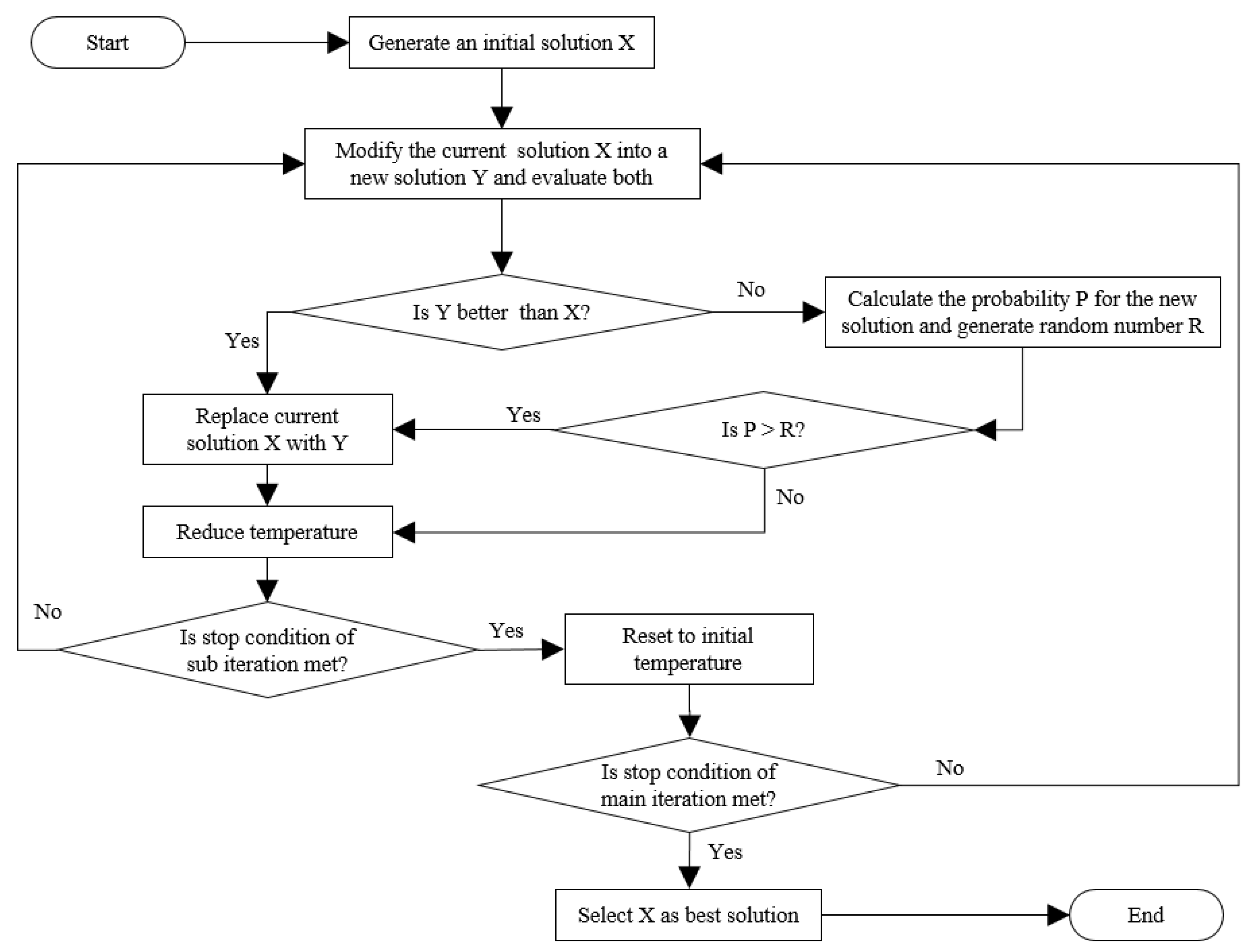
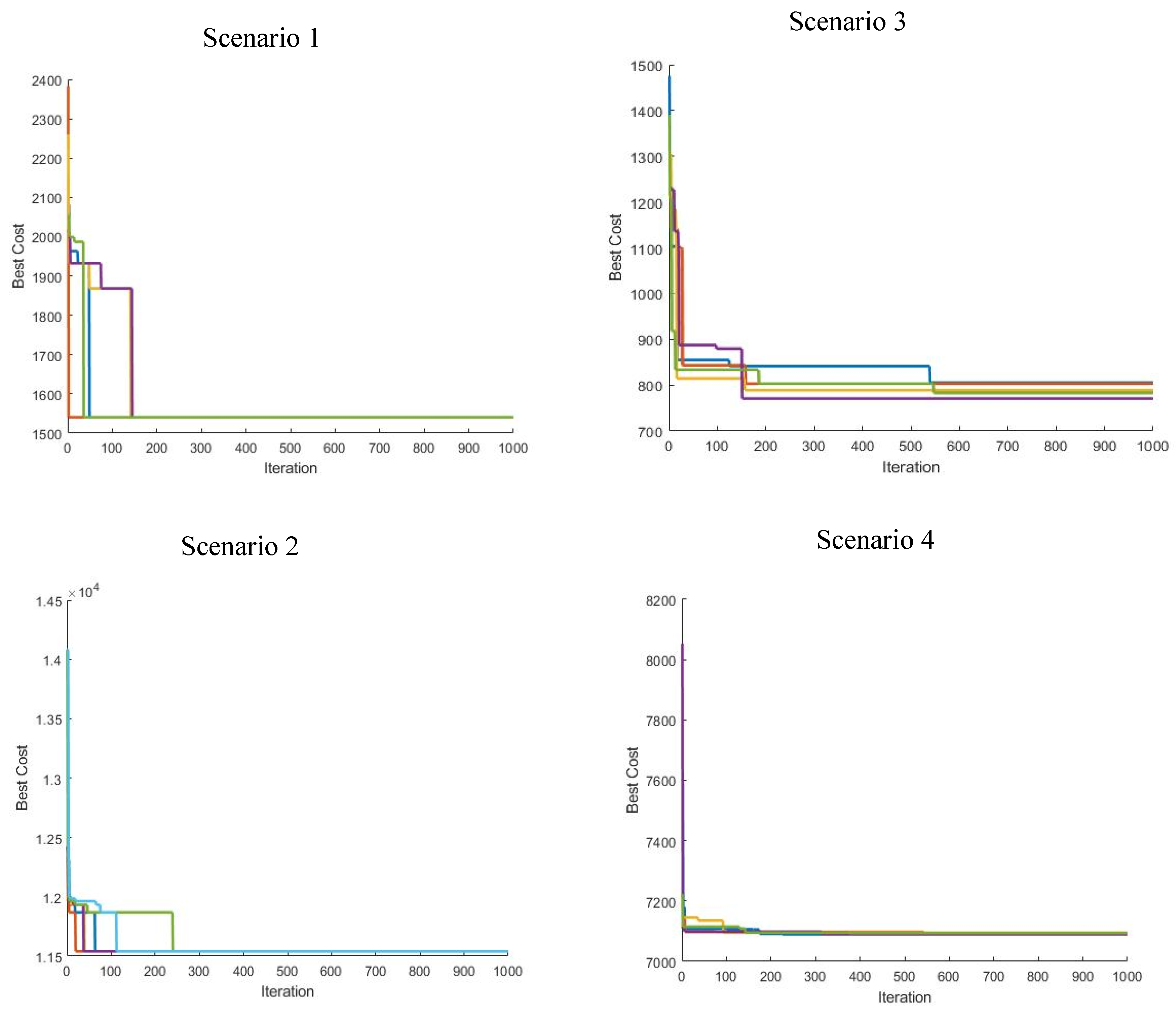
2.6. The Simulated Annealing Algorithm

The Simulated Annealing Algorithm (SAA) [17,18] is one of the most popular metaheuristic methods for solving combinatorial optimization problems. It simulates the physical process called annealing, where the properties of a material, typically a metal or an alloy, are improved by first heating the material and then slowly cooling it, causing a recrystallization of the molecular structure. The SAA algorithm simulates this process by going through a number of annealing iterations. The dynamics of the algorithm are controlled by a set of parameters (

Table 6. Parameters of simulated annealing algorithm (SAA).

Parameters	Values
Number of main iterations	1000
Number of sub iterations	60
Initial temperature	200
Temperature reduction rate	0.9

), such as the number of annealing iterations and the initial temperature of each iteration. For each annealing iteration, the temperature is reduced in a number of subiterations where the current temperature is multiplied with the temperature reduction rate (Table 6). The algorithm starts with an initial solution and for each subiteration it evaluates the current solution against a modified solution using the objective function, as illustrated in the flowchart of Figure 6.

In this application of SAA, the initial solution is a coverage of the field where the constraints are obeyed, so it consists of a set of tours where the total demand of the tracks of each tour is less than the bin capacity. For each subiteration, a new candidate solution is generated, e.g., by swapping tours. If the cost of the new solution is lower than the cost of the current, then the current solution will be replaced by the new. Even if the new solution is not better than the current one, they may be exchanged with a certain probability. In this way, the algorithm can escape a development towards a local optimum. The probability P is calculated with Equation (5), where T is the temperature and ∆C is the difference in cost of the solutions:

$$P=e^{-\Delta C/T}$$

(5)

Hence, the probability of exchanging with an inferior solution is highest in the beginning of an annealing iteration when the temperature is high or when the cost difference is low.

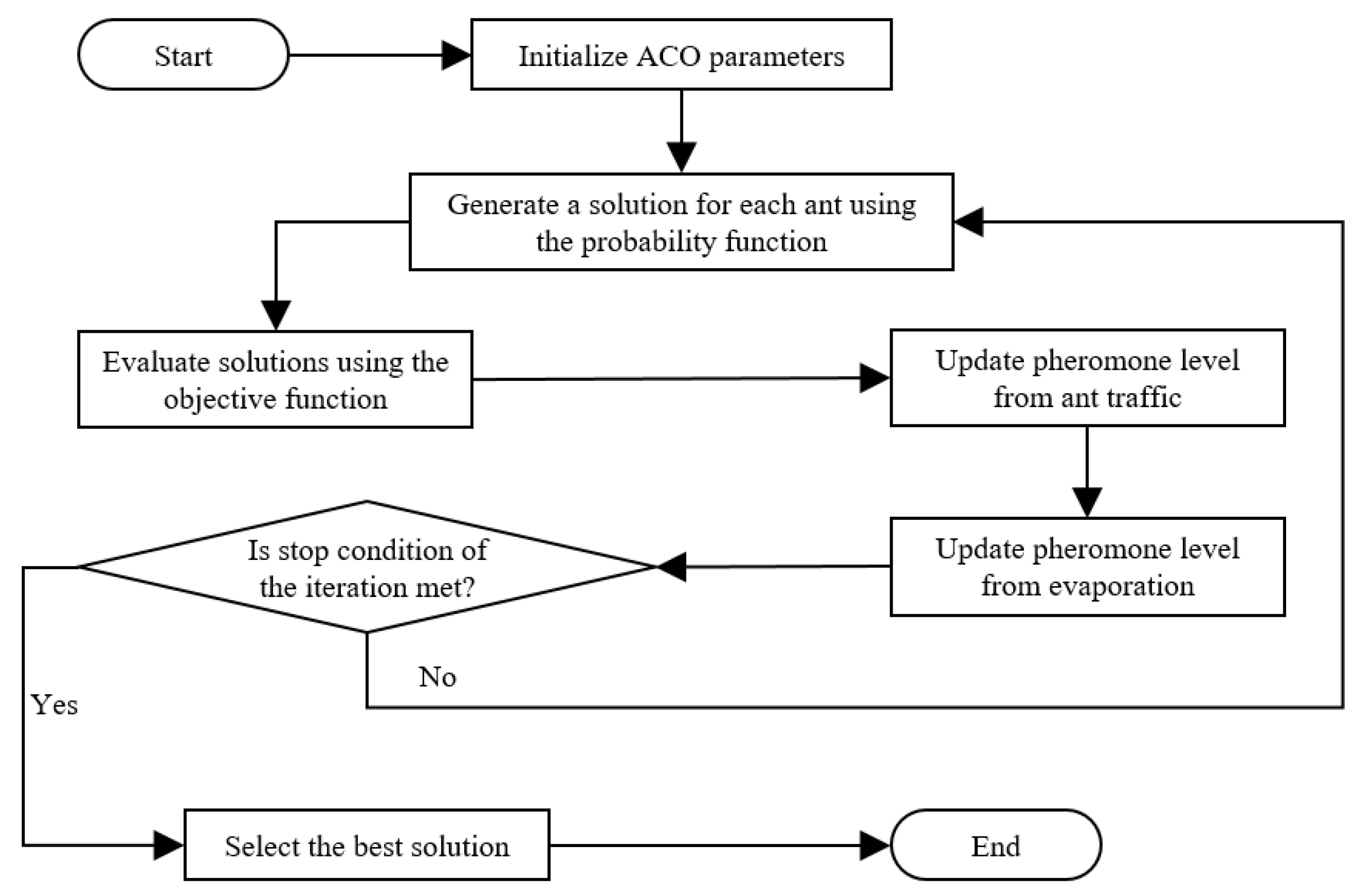
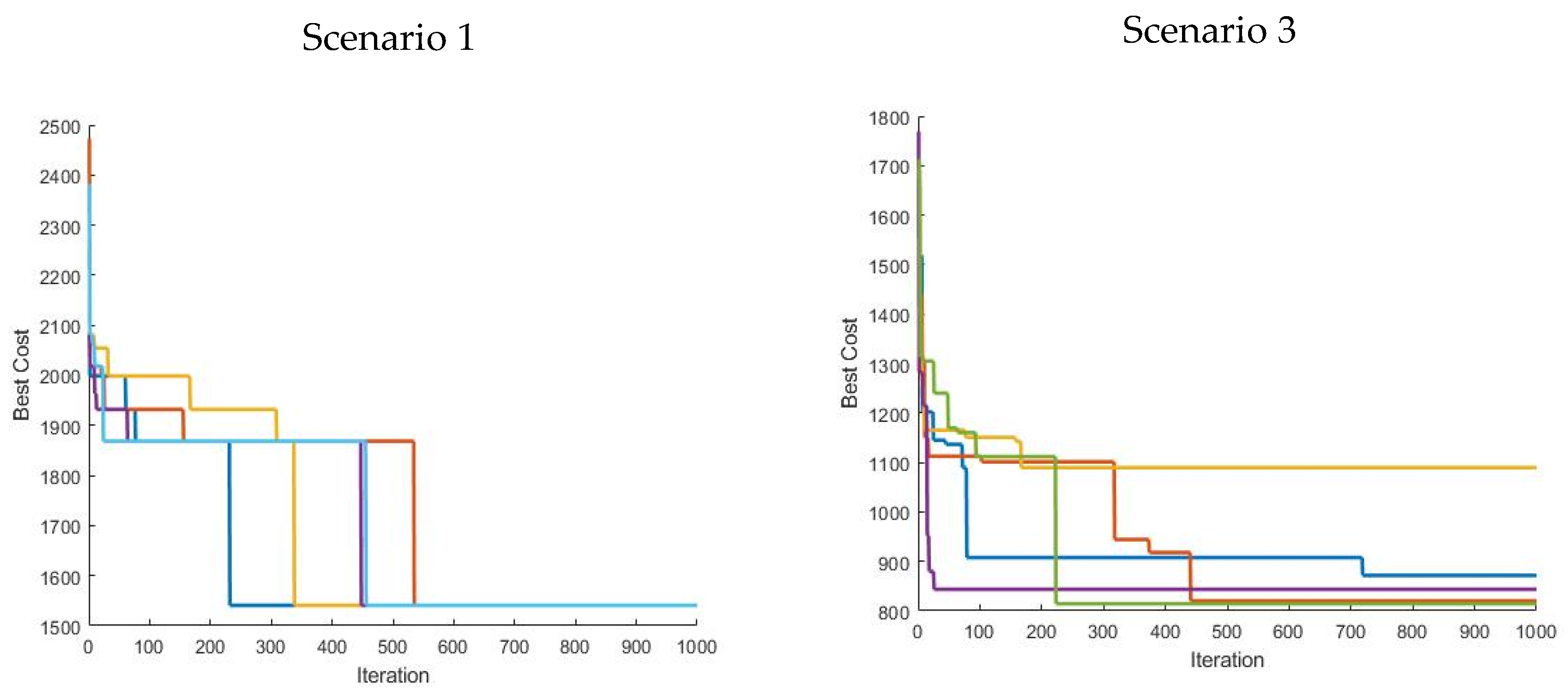
2.7. The Ant Colony Optimization Algorithm

The Ant Colony Optimization (ACO) algorithm is another metaheuristic method inspired by a phenomenon in nature and, as the name implies, it simulates the foraging behavior of ants. Individual ants roam out from the colony to find food, more or less randomly, and they leave a trail of pheromones. When other ants find such a trail, they are likely to follow it, hence enforcing the pheromone trail. The pheromone scent evaporates over time, so in this way the shortest way to the best food sources will gradually be travelled most and have the strongest pheromone scent. This ant behavior was first suggested as a metaheuristic optimization method by [32], and it has been applied in several types of optimization problems, including TSP [32] and capacitated VRP [21].

The ACO algorithm is governed by a set of parameters, shown in Table 8, including the number of ants and the number of iterations of the simulation. The flow of the algorithm is illustrated in Figure 7. Each ant will generate a solution in each iteration, based on information maintained by the algorithm. This information includes a pheromone matrix with elements τ_ij corresponding to the current pheromone level for the path from node i to j. The information also includes an “attractiveness” matrix with elements η_ij representing the value of alternative reasons than pheromone scent to move from node i to j. The attractiveness is defined here as the reciprocal value of the corresponding element in the cost matrix (Table A1 in Appendix A): η_ij = 1/C_ij. The main information for an ant to choose the next node is the probability function, which gives the probability, P_ij^k, that the kth ant will move from node i to node j. The probability is calculated as a combination of the level of pheromone and attractiveness of the move from i to j, where the relative influence of the two reasons are determined with the two weights α and β, respectively (

Table 7. Parameters of ant colony optimization (ACO).

Parameters	Values
Number of iterations	1000
Number of ants (population size)	60
Pheromone weight (α)	2
Attractiveness weight (β)	1
Evaporation rate ($\rho$)	0.01

). If j has been visited already by ant k then P_ij^k = 0, otherwise it should be calculated based on the following Equation (6):

$$p_{ij}^k=\frac{{\left({\tau }_{ij}\right)}^{\alpha }{\left({\eta }_{ij}\right)}^{\beta }}{{\sum }_z{\left({\tau }_{iz}\right)}^{\alpha }{\left({\eta }_{iz}\right)}^{\beta }}$$

(6)

where z is a member of the set of nodes not yet visited by ant k. When each ant has made a solution, its value is calculated with the objective function. Then the pheromone matrix is updated in two steps: scent from recent ant traffic is added and evaporation is subtracted from the scent. The value of the pheromone evaporation rate p is specified in Table 7.

3. Results and Discussion

3.1. Finding Distinct, Optimal Solutions

A significant part of the total theoretical number (${\mathcal{T}}_8$ = 1,321,205,760, see Table 1) of solutions for the benchmarking field with 8 tracks were not feasible, i.e., they contain one or more tours exceeding the bin capacity set in Table 3. For example, for scenario 1 (Table 5), only 116,613,120 solutions (9 pct.) were feasible. The non-working distance was calculated for all feasible solutions, and the minimum non-working distance was determined. For scenario 1, the minimum non-working distance turned out to be 1540.6 m, but (as shown in

Table 8. Number of absolute solutions before and after eliminating different combinations.

Scenario	Number of Absolute Solutions	Number of Absolute Solutions after Eliminating Different Combinations	Number of Unique, Absolute Solutions
1	3840	32	1
2	3840	32	1
3	384	16	1
4	96	16	2

) 3840 solutions had this minimum non-working distance, so they were all absolute solutions.

Not all 3840 absolute solutions were distinct; however, two solutions consisting of the same set of tours, but with different ordering of the tours, are considered equivalent. Figure 8 illustrates how equivalent solutions can be made as a combination of the same five tours. This type of equivalence reduced the set of solutions to 32.

Moreover, two tours are considered equivalent if they consist of the same paths in revered order, since this will result in a similar driving pattern with the same non-working distance. For example, the tours [0, 3, 14, 0] and [0, 13, 4, 0] are equivalent, as shown in Figure 9. Thereby, the number of absolute solutions are reduced to one or two unique solutions by removing solutions that contain the same paths with reversed order.

In this way, all 3840 solutions for Scenario 1 with non-working distance 1540.6 m turned out to be equivalent. Likewise, Scenarios 2 and 3 have one unique, absolute solution each, while Scenario 4 has two distinct, absolute solutions, as shown in

Table 9. Unique, absolute solutions and corresponding non-working distances.

Scenario	Non-Working (m)	Absolute Solution(s)
1	1540.6	[0, 1, 12, 0, 3, 10, 0, 5, 8, 0, 14, 0, 16, 0]
2	11,540.6	[0, 1, 12, 0, 3, 10, 0, 5, 8, 0, 14, 0, 16, 0]
3	745.0	[0, 1, 4, 0, 5, 8, 0, 9, 12, 0, 13, 16, 0]
4	7085.5	[0, 2, 5, 12, 0, 4, 7, 10, 0, 13, 16, 0] [0, 1, 5, 12, 0, 4, 7, 10, 0, 13, 16, 0]

and

Table 10. Unique, absolute solutions and corresponding non-working distances.

	SAA			ACO
Scenario	Non-Working Distance (m)	Execution Time (s)	Solution	Non-Working Distance (m)	Execution Time (s)	Solution
1	1540.6	50 < t < 60	[0, 1, 12, 0, 3, 10, 0, 5, 8, 0, 14, 0, 16, 0]	1540.6	105 < t < 120	[0, 1, 12, 0, 3, 10, 0, 5, 8, 0, 14, 0, 16, 0]
2	11,540.6	50 < t < 60	[0, 1, 12, 0, 3, 10, 0, 5, 8, 0, 14, 0, 16, 0]	11,540.6	105 < t < 120	[0, 1, 12, 0, 3, 10, 0, 5, 8, 0, 14, 0, 16, 0]
3	771.0	35 < t < 45	[0, 1, 6, 0, 3, 8, 0, 9, 12, 0, 13, 16, 0]	814.3	75 < t < 85	[0, 1, 4, 0, 5, 14, 0, 7, 10, 0, 11, 16, 0]
4	7089.5	35 < t < 45	[0, 1, 7, 12, 0, 9, 4, 6, 0, 13, 16, 0]	7095.0	75 < t < 85	[0, 1, 7, 12, 0, 5, 4, 10, 0, 13, 16, 0]

.

It is obvious that when using the machine with large bin capacity the field can be covered with fewer tours, saving transport between field and depot. Table 9 shows that the absolute solution is the same for Scenarios 1 and 2 when the bin capacity is 30,000 L, so in both cases, the solution has five tours. Therefore, the 10,000 m difference in non-working distance between the two scenarios stems from the additional distance to the depot and back five times. The absolute solutions are different when the machine’s bin capacity is 46,000 L (Scenarios 3 and 4) and the number of tours is reduced to four and three, respectively. Interestingly, even though the large bin capacity enables the field to be covered in three tours, this is only optimal when the depot is sufficiently far away, due to additional driving inside the field.

3.2. Near-Optimal Solutions of Metaheuristic Algorithms

The two metaheuristic algorithms, SAA and ACO, were applied repeatedly with the input parameters defined in Table 6 and Table 7, respectively. Since they are probabilistic methods, the outcome is different for each execution. Table 10 shows the solutions with minimal non-working distance found by the two metaheuristic algorithms in up to 1000 iterations. Neither of the algorithms was able to find the absolute solution for Scenarios 3 and 4, but both succeeded for Scenarios 1 and 2 (Table 10). It may be a little surprising that for two scenarios both algorithms failed to find the optimum for the relatively simple field with only eight tracks in 1000 attempts, but this also illustrates the complexity of the NP-hard problem. Both algorithms have found solutions with non-working distance close to the optimum value; however, these are up to 6 pct longer than the optimum and with SAA getting closer than ACO. The probability of a metaheuristic algorithm to find an optimal solution will decrease with the size of the solution space, so, likely, the algorithms will not find the optimal solution in larger fields. In addition to the size, the shape of fields also affects the chances of finding the absolute solution. A field with close to rectangular shape will have many optimal solutions in the search space, since the tracks have a similar length, increasing the chances that one will be found by the algorithm. Alternatively, fields with large variation in the length of tracks will have fewer absolute solutions, thus reducing the chances of finding one by the metaheuristic algorithms. Finally, a larger bin capacity increases the number of feasible solutions, as more tracks can be covered per tour, and hence reduces the chances of the algorithms to reach optimum. The results in Table 10 support this fact, as both algorithms found the absolute solution with the smaller bin capacity, but not with the larger.

Comparing the two metaheuristic algorithms (Table 10), SAA is performing better than ACO. The non-working distance of the found solutions are equal or slightly lower for SAA, but they are found in roughly half the time. The values of execution time in Table 10 are a range of seconds, since the algorithms were executed multiple times.

3.3. Convergence towards Optimum

Figure 10 and Figure 11 show a comparison of the optimization process of the two metaheuristic algorithms: SAA in Figure 10 and ACO in Figure 11. Each figure shows a plot for each scenario, where the cost of the currently best solution of an algorithm is plotted against the iteration number for five repetitions of the algorithm. Each repetition in a plot is shown with a colored stepwise curve, where the curve is piecewise horizontal until it reaches an iteration when a solution with a lower cost has been found, causing a step down of the curve to a lower level. Figure 10 shows that for scenarios 1 and 2 SAA could reach the absolute solution in less than 250 iterations for all five repetitions. For Scenarios 3 and 4 the larger bin capacity results in a larger search space, so we expected a slower convergence towards the absolute solution. This is indeed the case for Scenario 3, but not for Scenario 4. The reason for the fast convergence towards a local optimum in scenario 4 is that there are only 96 absolute solutions for this scenario, according to Table 9. Therefore, it is more difficult for the algorithms to find an absolute solution and stuck with a local optimum.

Figure 11 shows that the convergence is slower for the ACO algorithm, relative to SAA in Figure 10. There is also a larger variation between the five repetitions than we saw for SAA. For example, in Scenario 2, one repetition of ACO found the absolute solution in less than 100 iterations, while another repetition required more than 900 iterations to find it.

Knowing the global optimum solution for a benchmark field can be helpful to better evaluate the performance and the quality of the solution for a developed algorithm. As it mentioned before, there are several functions and datasets which can be used for testing and evaluating the optimization algorithms [22,23,24,25]. However, none of them provide an absolute optimum solution for those datasets. The presented field in this study can be used as a good benchmark for the evaluation of the quality of the solution gained by metaheuristic algorithms.

As the limitations of this study, it was necessary to have a powerful computer with considerable amount of RAM capacity to accomplish all the calculations. Due to the huge size of the solution space for this problem, even for a small field with eight tracks, finding the global optimum solution was challenging with a normal computer (Intel^® Core™ i7-7700 [email protected] with 24 GB RAM).

As future research, it is possible to use more powerful computers with several GPUs in order to find the absolute optimal solution for a bigger field (with more tracks). Furthermore, the other criteria (apart from the non-working traveled distance) such as process time, fuel consumption, or soil compaction can also be considered for the evaluation of the solution. Moreover, it is possible to use the presented global optimum coverage path in this study for the UAV’s application.

4. Conclusions

Metaheuristic algorithms for finding the most efficient route for agricultural operations covering a field were evaluated in terms of efficiency and optimality. The basis for the evaluation was the selection and specification of an agricultural field for benchmarking the multiple metaheuristic algorithms against an exhaustive optimality calculation. The field was specified as a 2.97 hectare field in Denmark with eight tracks of different lengths. The field was selected for being sufficiently simple (few tracks) to determine the exhaustive global optimum, i.e., the solution with the shortest non-working distance, and at the same time sufficiently complex (different track lengths) for metaheuristic algorithms to have difficulty in finding the global optimum. The total number of different ways to cover this field by traversing the eight tracks for a capacitated operation is 1,321,205,760. Not all of those potential solutions are feasible since this depends on the bin capacity of the machine and the demand for tracks of the specific capacitated operation. Four scenarios were specified as a combination of low/high bin capacity and short/long distance between field and depot. For each scenario, the global optimum and the corresponding cost value (non-working distance) were determined. Each scenario had multiple (thousands) optimal solutions, but with one exception they were all equivalent, i.e., permutations of the same tours and of tours where the tracks were visited in the opposite order. The exception was one scenario with two unique, absolute optimal solutions.

Two metaheuristic algorithms, Ant Colony Optimization (ACO) and Simulated Annealing Algorithm (SAA) were selected for benchmarking using the specified benchmarking field. Each algorithm was applied to each scenario. For the two scenarios with low bin capacity both algorithms managed to find the absolute solution, while for the two scenarios with high bin capacity, they came close to the absolute solution, with ASS marginally better. However, the execution time of ACO was around twice the time of ASS, and ACO showed more variation in the quality of the best solution. In conclusion, ASS performed better than ACO in the benchmarking test.

As future research, it is possible to use more powerful computers with several GPUs in order to find the absolute optimal solution for a bigger field (with more tracks). Furthermore, the other criteria (apart from the non-working traveled distance) such as process time, fuel consumption, or soil compaction can also be considered for the evaluation of the solution. Moreover, it is possible to use the presented global optimum coverage path in this study for the UAV’s application.

References

1. Xie, J.; Carrillo, L.; Jin, L. An Integrated Traveling Salesman and Coverage Path Planning Problem for Unmanned Aircraft Systems. IEEE Control Syst. Lett. 2019, 3, 67–72. [Google Scholar] [CrossRef]
2. Plessen, M.G. Coupling of crop assignment and vehicle routing for harvest planning in agriculture. Artif. Intell. Agric. 2019, 2, 99–109. [Google Scholar] [CrossRef]
3. Torres, M.; Pelta, D.; Verdegay, J.; Torres, J. Coverage path planning with unmanned aerial vehicles for 3D terrain reconstruction. Expert Syst. Appl. 2016, 55, 441–451. [Google Scholar] [CrossRef]
4. Conesa-Muñoz, J.; Pajares, G.; Ribeiro, A. Mix-opt: A new route operator for optimal coverage path planning for a fleet in an agricultural environment. Expert Syst. Appl. 2016, 54, 364–378. [Google Scholar] [CrossRef]
5. Khajepour, A.; Sheikhmohammady, M.; Nikbakhsh, E. Field path planning using capacitated arc routing problem. Comput. Electron. Agric. 2020, 173, 105401. [Google Scholar] [CrossRef]
6. Edwards, G.; Jensen, M.; Bochtis, D. Coverage planning for capacitated field operations under spatial variability. Int. J. Sustain. Agric. Manag. Inform. 2015, 1, 120. [Google Scholar] [CrossRef]
7. Hameed, I.A.; Bochtis, D.D.; Sorensen, C.G. Driving Angle and Track Sequence Optimization for Operational Path Planning Using Genetic Algorithms. Appl. Eng. Agric. 2011, 27, 1077–1086. [Google Scholar] [CrossRef]
8. Jin, J.; Tang, L. Optimal Coverage Path Planning for Arable Farming on 2D Surfaces. Trans. ASABE 2010, 53, 283–295. [Google Scholar] [CrossRef]
9. Li, Y.; Yi, S. Improving the efficiency of spatially selective operations for agricultural robotics in cropping field. Span. J. Agric. Res. 2013, 11, 56. [Google Scholar] [CrossRef] [Green Version]
10. Jensen, M.F.; Bochtis, D.; Sørensen, C.G. Coverage planning for capacitated field operations, part II: Optimisation. Biosyst. Eng. 2015, 139, 149–164. [Google Scholar] [CrossRef]
11. Baldacci, R.; Mingozzi, A.; Roberti, R. Recent exact algorithms for solving the vehicle routing problem under capacity and time window constraints. Eur. J. Oper. Res. 2012, 218, 1–6. [Google Scholar] [CrossRef]
12. Shi, Y.; Lv, L.; Hu, F.; Han, Q. A Heuristic Solution Method for Multi-Depot Vehicle Routing-Based Waste Collection Problems. Appl. Sci. 2020, 10, 2403. [Google Scholar] [CrossRef] [Green Version]
13. Shen, J.; Shigeoka, K.; Ino, F.; Hagihara, K. GPU-based branch-and-bound method to solve large 0-1 knapsack problems with data-centric strategies. Concurr. Comput. 2019, 31, e4954. [Google Scholar] [CrossRef]
14. Cao, C.; Li, C.; Yang, Q.; Zhang, F. Multi-Objective Optimization Model of Emergency Organization Allocation for Sustainable Disaster Supply Chain. Sustainability 2017, 9, 2103. [Google Scholar] [CrossRef] [Green Version]
15. Yuliza, E.; Puspita, F. The Branch and Cut Method for Solving Capacitated Vehicle Routing Problem (CVRP) Model of LPG Gas Distribution Routes. Sci. Technol. Indones. 2019, 4, 105. [Google Scholar] [CrossRef] [Green Version]
16. Pamosoaji, A.K.; Dewa, P.K.; Krisnanta, J.V. Proposed Modified Clarke-Wright Saving Algorithm for Capacitated Vehicle Routing Problem. Int. J. Ind. Eng. Eng. Manag. 2019, 1, 9. [Google Scholar] [CrossRef]
17. Chokanat, P.; Pitakaso, R.; Sethanan, K. Methodology to Solve a Special Case of the Vehicle Routing Problem: A Case Study in the Raw Milk Transportation System. AgriEngineering 2019, 1, 75–93. [Google Scholar] [CrossRef] [Green Version]
18. Vahdanjoo, M.; Madsen, C.T.; Sørensen, C.G. Novel Route Planning System for Machinery Selection. Case: Slurry Application. AgriEngineering 2020, 2, 408–429. [Google Scholar] [CrossRef]
19. Sbai, I.; Limam, O.; Krichen, S. An effective genetic algorithm for solving the capacitated vehicle routing problem with two-dimensional loading constraint. Int. J. Comput. Intell. Stud. 2020, 9, 85. [Google Scholar] [CrossRef]
20. Akbar, M.D.; Aurachmana, R. Hybrid genetic–tabu search algorithm to optimize the route for capacitated vehicle routing problem with time window. Int. J. Ind. Optim. 2020, 1, 15–28. [Google Scholar] [CrossRef] [Green Version]
21. Kanso, B. Hybrid ANT Colony Algorithm for the Multi-depot Periodic Open Capacitated Arc Routing Problem. Int. J. Artif. Intell. Appl. Jan. 2020, 11, 53–64. [Google Scholar] [CrossRef] [Green Version]
22. Peng, F.M. Novel composition test functions algorithm for numerical optimization. In Proceedings of the 2011 International Conference on Computer Science and Service System (CSSS), Nanjing, China, 27–29 June 2011; pp. 3348–3352. [Google Scholar]
23. Okabe, T.; Jin, Y.; Olhofer, M.; Sendhoff, B. On test functions for evolutionary multi-objective optimization. In Parallel Problem Solving from Nature—PPSN VIII; Lecture Notes in Computer Science (including subseries Lecture Notes in Artificial Intelligence and Lecture Notes in Bioinformatics); Springer: Berlin/Heidelberg, Germany, 2004; Volume 3242, pp. 792–802. [Google Scholar]
24. Laguna, M.; Martí, R. Experimental testing of advanced scatter search designs for global optimization of multimodal functions. J. Glob. Optim. 2005, 33, 235–255. [Google Scholar] [CrossRef]
25. Guo, Y.; Zhang, L.; Hu, Y.; He, X.; Gao, J. MS-celeb-1M: A dataset and benchmark for large-scale face recognition. Lect. Notes Comput. Sci. 2016, 9907, 87–102. [Google Scholar]
26. Bochtis, D.D.; Sørensen, C.G.; Busato, P.; Berruto, R. Benefits from optimal route planning based on B-patterns. Biosyst. Eng. 2013, 115, 389–395. [Google Scholar] [CrossRef]
27. Bochtis, D.; Sørensen, C. The vehicle routing problem in field logistics part I. Biosyst. Eng. 2009, 104, 447–457. [Google Scholar] [CrossRef]
28. Bochtis, D.D.; Sørensen, C.G. The vehicle routing problem in field logistics: Part II. Biosyst. Eng. 2010, 105, 180–188. [Google Scholar] [CrossRef]
29. Bochtis, D.D.; Vougioukas, S.G. Minimising the non-working distance travelled by machines operating in a headland field pattern. Biosyst. Eng. 2008, 101, 1–12. [Google Scholar] [CrossRef]
30. Savla, K.; Frazzoli, E.; Bullo, F. Traveling Salesperson Problems for the Dubins Vehicle. IEEE Trans. Autom. Control. 2008, 53, 1378–1391. [Google Scholar] [CrossRef]
31. Möhring, R.H.; Schilling, H.; Schütz, B.; Wagner, D.; Willhalm, T. Partitioning graphs to speed up Dijkstra’s algorithm. ACM J. Exp. Algorithmics 2006, 11, 2–8. [Google Scholar]
32. Gambardella, L.M.; Dorigo, M. Solving symmetric and asymmetric TSPs by ant colonies. In Proceedings of the IEEE Conference on Evolutionary Computation, Nagoya, Japan, 20–22 May 1996; pp. 622–627. [Google Scholar]
Figure 1. Illustration of the number of permutations for eight tracks with two driving directions for each track.
Agronomy 10 01454 g001
Figure 2. The number of solutions TN as a function of the number of tracks N.
Agronomy 10 01454 g002
Figure 3. Google Earth picture of the selected benchmarking field with indications of the location of the depot (D) and the field polygon (yellow lines) with 5 corners (red markers 1 to 5).
Agronomy 10 01454 g003
Figure 4. Geometrical representation of the field with depot, tracks, and turnings (not all possible turnings between tracks are shown).
Agronomy 10 01454 g004
Figure 5. IDs of endpoints of each track.
Agronomy 10 01454 g005
Figure 6. Flowchart of the simulated annealing algorithm (SAA).
Agronomy 10 01454 g006
Figure 7. Flowchart of the Ant Colony Optimization (ACO) algorithm.
Agronomy 10 01454 g007
Figure 8. Example of equivalent solutions consisting of the same 5 tours in different combinations.
Agronomy 10 01454 g008
Figure 9. Two equivalent tours (red and black) containing the same paths with reversed order.
Agronomy 10 01454 g009
Figure 10. The cost of the best solution for each iteration of SAA. Each color is a separate execution of the algorithm.
Agronomy 10 01454 g010
Figure 11. The cost of the best solution for each iteration of ACO. Each color is a separate execution of the algorithm.
Agronomy 10 01454 g011aAgronomy 10 01454 g011b