Comparing Apple and Pear Phenology and Model Performance: What Seven Decades of Observations Reveal


Abstract
1. Introduction
2. Materials and Methods
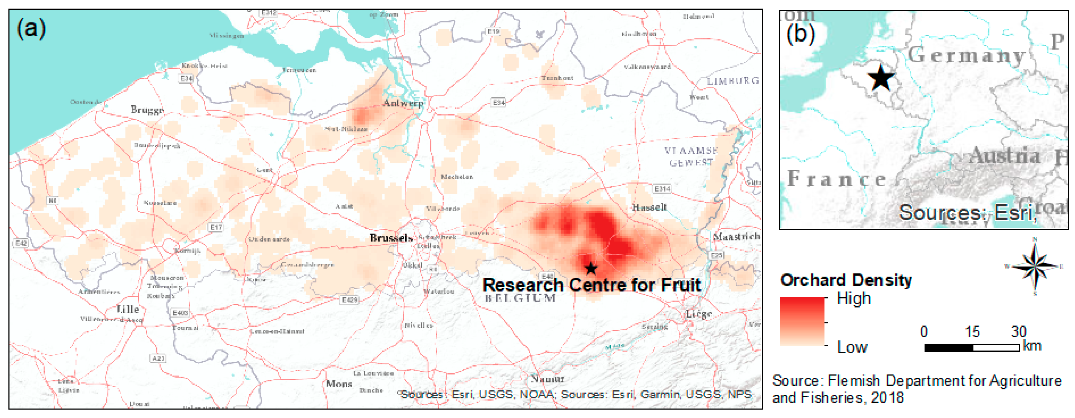
2.1. Study Area
2.2. Phenology and Meteorology
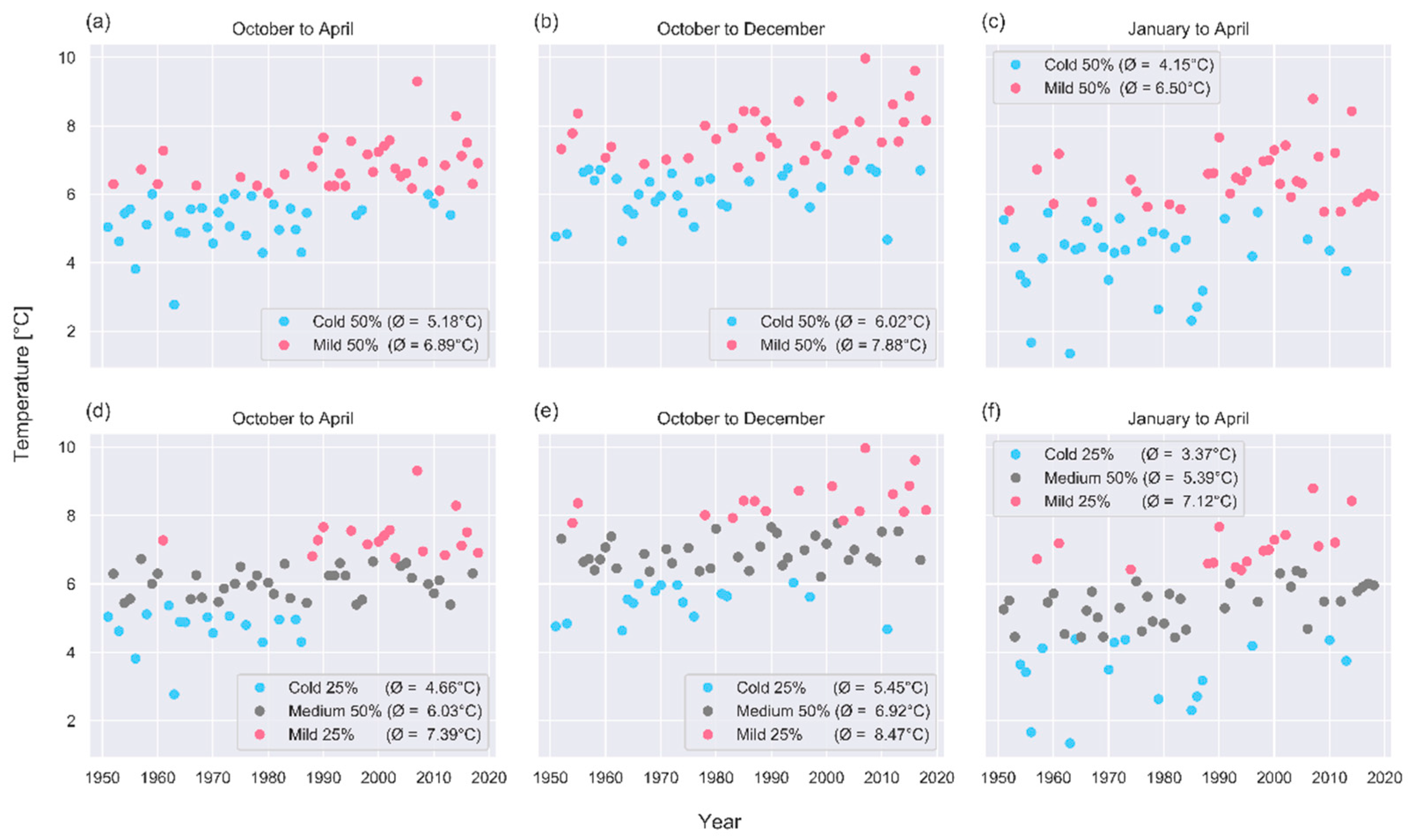
2.3. Ranking Observations to Derive Past Change Signals
2.4. Partial Least Square Regression
2.5. Phenological Models
2.5.1. Continuous Model
2.5.2. Dynamic + GDH Model
2.5.3. Parameter Optimization
3. Results
3.1. Past Change Signals
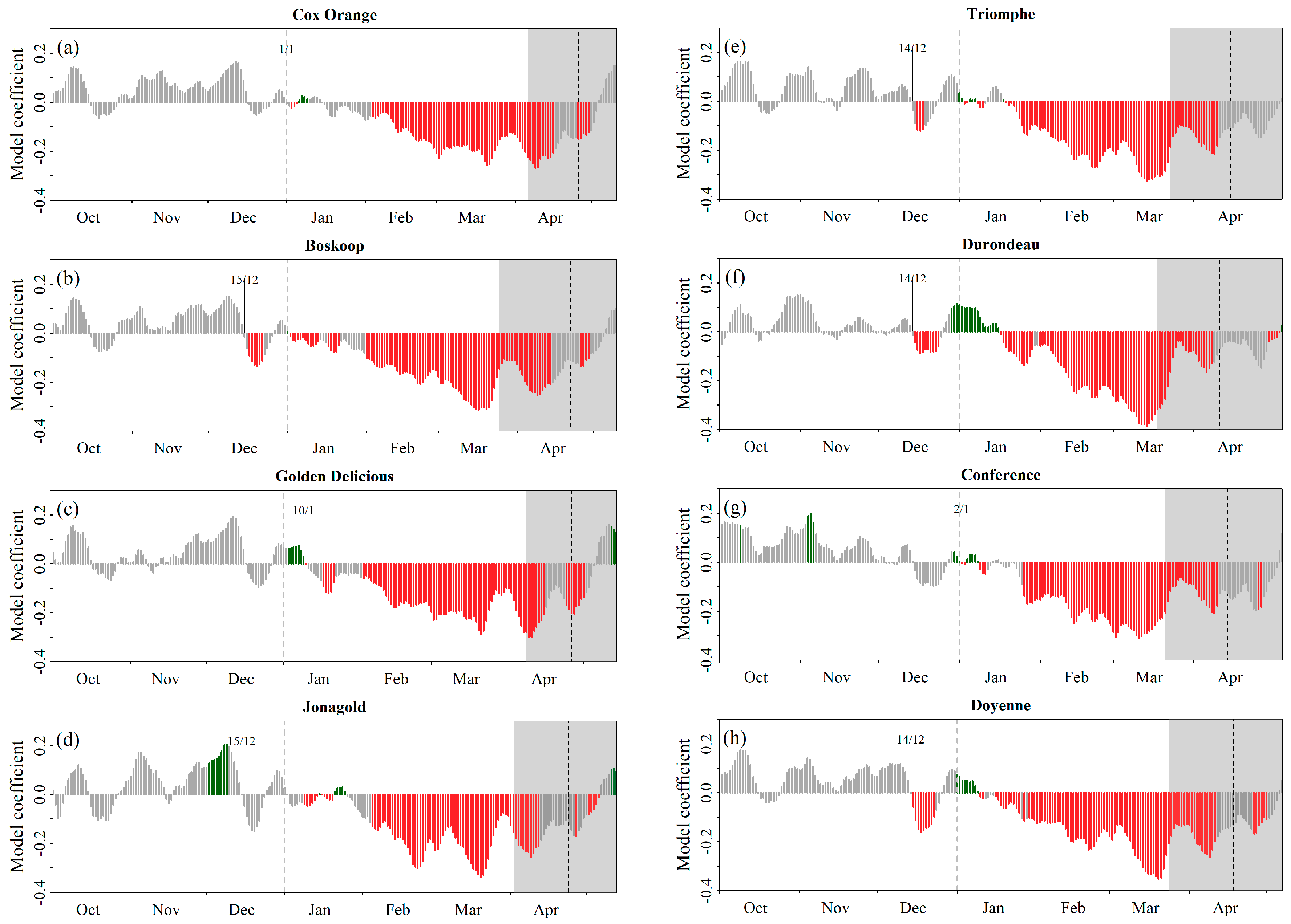
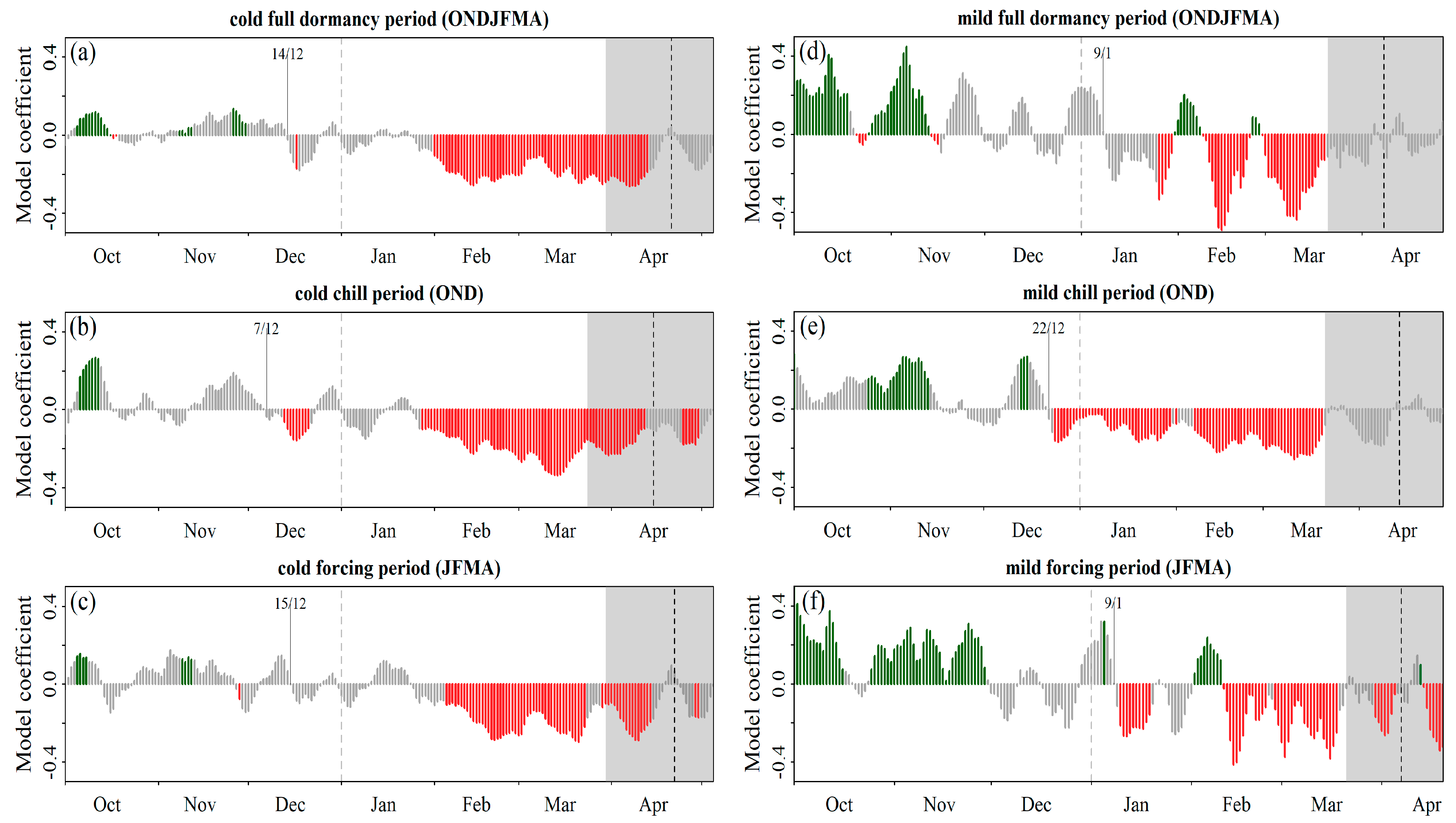
Phenological Response to Warming: Partial Least Square Regression
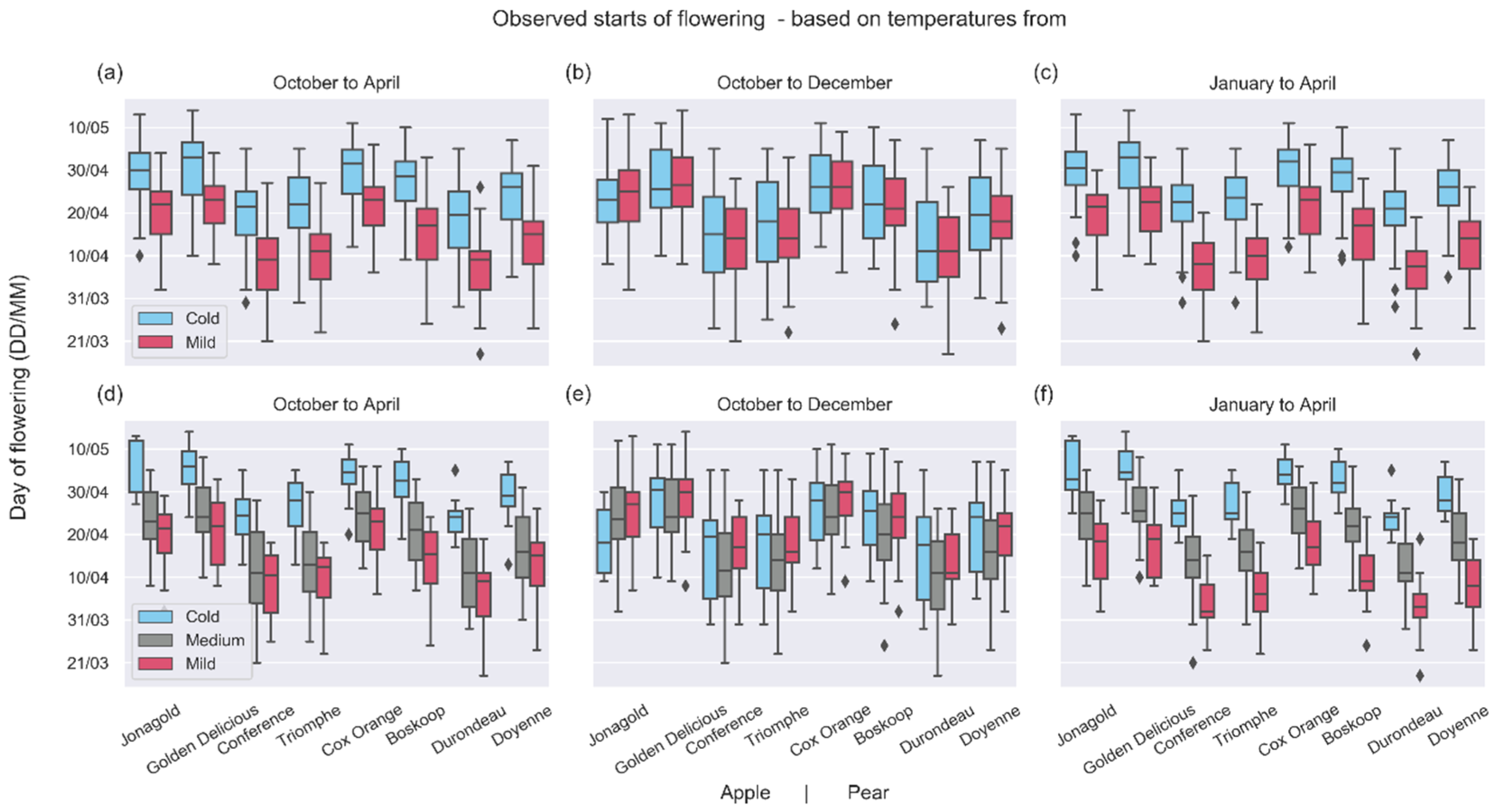
3.2. Shifts of Phenological Phases
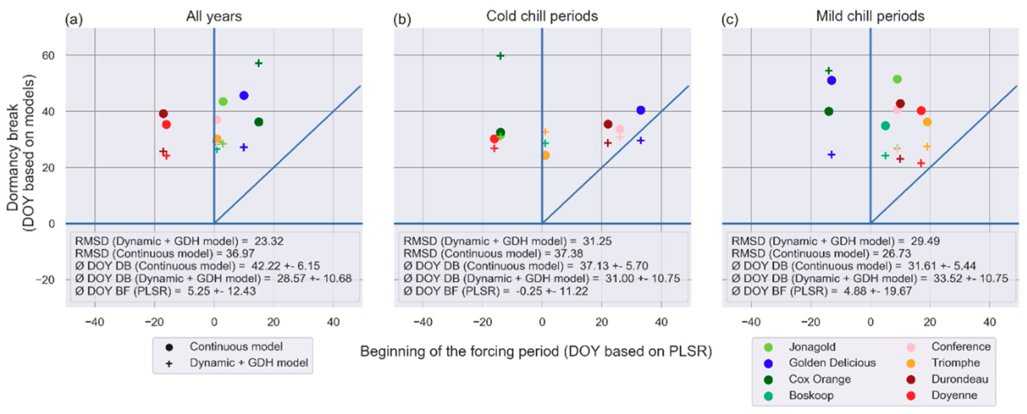
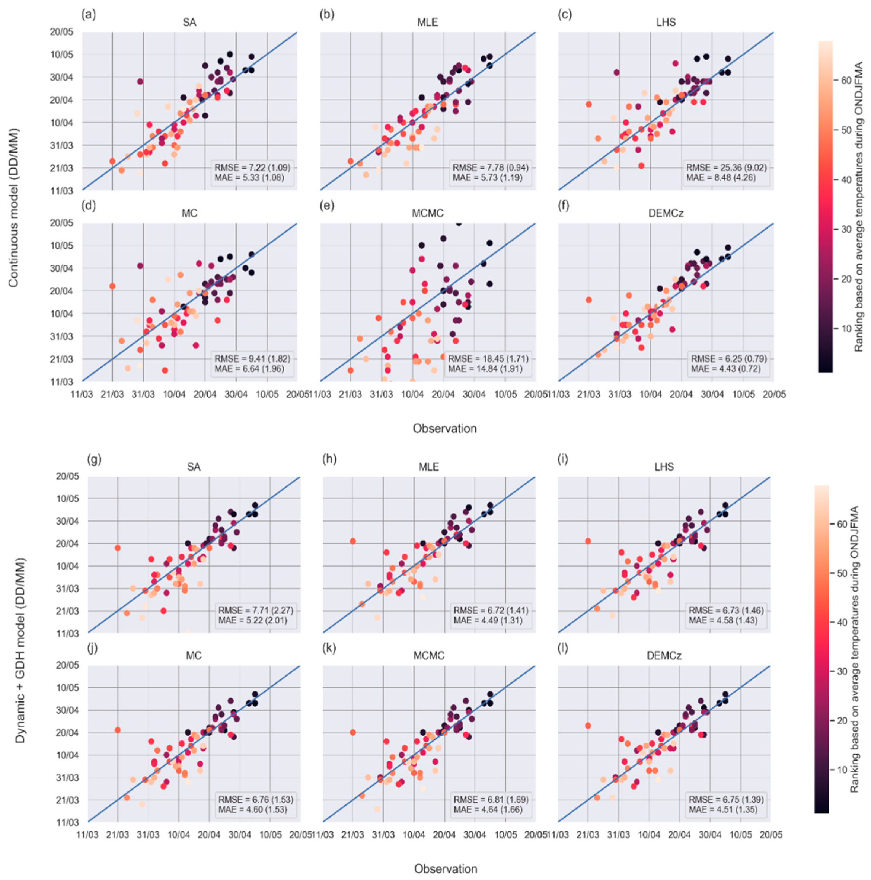
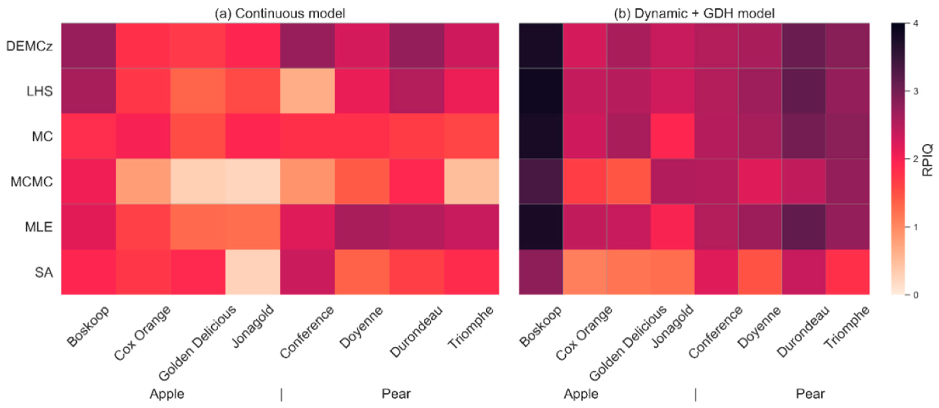
3.3. Phenological Models: Sensitivity of Predictions to the Model and to the Parameter Calibration Algorithm
4. Discussion
4.1. Past Change Signals
Phenological Response to Warming: Partial Least Square Regression
4.2. Shifts in Phenological Phases
4.3. Evaluation of the Phenological Models
5. Conclusions
Author Contributions
Funding
Acknowledgments
Conflicts of Interest
Appendix A

| Cultivar | Algorithm | C | TBc | TBf | Tup | a | b | Calibration | RMSE Validation | Mean |
|---|---|---|---|---|---|---|---|---|---|---|
| Boskoop | DEMCz | 41.84 | 2.00 | 5.00 | 10.87 | 140.00 | −0.001 | 6.28 | 5.43 | 5.85 |
| Cox Orange | MC | 54.10 | 2.91 | 5.74 | 12.64 | 162.00 | −0.00584 | 5.90 | 6.15 | 6.03 |
| Golden D. | SA | 48.44 | 3.61 | 4.77 | 10.38 | 170.00 | −0.00392 | 6.31 | 6.47 | 6.39 |
| Jonagold | DEMCz | 40.00 | 4.69 | 5.00 | 9.17 | 192.20 | −0.00736 | 7.32 | 4.80 | 6.06 |
| Conference | DEMCz | 59.44 | 2.00 | 4.61 | 13.95 | 214.50 | −0.01 | 4.15 | 7.76 | 5.96 |
| Doyenne | MLE | 50.00 | 2.00 | 4.68 | 12.14 | 214.20 | −0.01 | 4.98 | 5.73 | 5.36 |
| Durondeau | DEMCz | 62.44 | 4.65 | 4.71 | 14.00 | 214.20 | −0.01 | 6.02 | 6.34 | 6.18 |
| Triomphe | MLE | 42.72 | 3.84 | 4.60 | 10.51 | 203.80 | −0.011505 | 6.55 | 6.03 | 6.29 |
| Cultivar | Algorithm | CR | HR | Calibration | RMSE Validation | Mean |
|---|---|---|---|---|---|---|
| Boskoop | LHS | 59.16 | 4430 | 4.10 | 4.20 | 4.15 |
| Cox Orange | LHS | 79.6 | 4268 | 4.21 | 5.70 | 4.95 |
| Golden Delicious | MC | 59.84 | 4980 | 4.08 | 5.12 | 4.60 |
| Jonagold | MCMC | 60.66 | 4644 | 4.85 | 4.57 | 4.71 |
| Conference | DEMCz | 60.6 | 3484 | 4.48 | 8.39 | 6.43 |
| Doyenne | MLE | 57.62 | 4184 | 3.54 | 6.35 | 4.95 |
| Durondeau | MLE | 58.66 | 3464 | 3.88 | 6.50 | 5.19 |
| Triomphe | DEMCz | 61.38 | 3632 | 4.48 | 5.98 | 5.23 |
References
- Farm and Horticultural Holdings|Statbel. Available online: http://statbel.fgov.be/en/themes/agriculture-fishery/farm-and-horticultural-holdings (accessed on 3 July 2019).
- WAPA. European Apple and Pear Crop Forecast; World Apple and Pear Organisation: Brussles, Belgium, 2018. [Google Scholar]
- Faust, M.; Erez, A.; Rowland, L.J.; Wang, S.Y.; Norman, H.A. Bud Dormancy in Perennial Fruit Trees: Physiological Basis for Dormancy Induction, Maintenance, and Release. HortScience 1997, 32, 623–629. [Google Scholar] [CrossRef]
- Anderson, J.L.; Richardson, E.A.; Kesner, C.D. Validation of chill unit and flower bud phenology models for “Montmorency” sour cherry. Acta Hortic. 1986, 184, 71–78. [Google Scholar] [CrossRef]
- Luedeling, E. Climate change impacts on winter chill for temperate fruit and nut production: A review. Sci. Hortic. 2012, 144, 218–229. [Google Scholar] [CrossRef]
- Fishman, S.; Erez, A.; Couvillon, G.A. The temperature dependence of dormancy breaking in plants: Computer simulation of processes studied under controlled temperatures. J. Theor. Biol. 1987, 126, 309–321. [Google Scholar] [CrossRef]
- Hänninen, H. Modelling bud dormancy release in trees from cool and temperate regions. Acta For. Fenn. 1990. [Google Scholar] [CrossRef]
- Chmielewski, F.-M.; Blümel, K.; Henniges, Y.; Blanke, M.; Weber, R.W.S.; Zoth, M. Phenological models for the beginning of apple blossom in Germany. Meteorol. Z. 2011, 20, 487–496. [Google Scholar] [CrossRef]
- Luedeling, E.; Brown, P.H. A global analysis of the comparability of winter chill models for fruit and nut trees. Int. J. Biometeorol. 2011, 55, 411–421. [Google Scholar] [CrossRef]
- Luedeling, E.; Gassner, A. Partial Least Squares Regression for analyzing walnut phenology in California. Agric. For. Meteorol. 2012, 158–159, 43–52. [Google Scholar] [CrossRef]
- Unterberger, C.; Brunner, L.; Nabernegg, S.; Steininger, K.W.; Steiner, A.K.; Stabentheiner, E.; Monschein, S.; Truhetz, H. Spring frost risk for regional apple production under a warmer climate. PLoS ONE 2018, 13, e0200201. [Google Scholar] [CrossRef]
- Brunner, L.; Hegerl, G.C.; Steiner, A.K. Connecting Atmospheric Blocking to European Temperature Extremes in Spring. J. Clim. 2016, 30, 585–594. [Google Scholar] [CrossRef]
- Legave, J.-M.; Guédon, Y.; El Yaacoubi, A.; Malagi, G.; Mathieu, V.; Christien, D.; Farrera, I.; Bonhomme, M. Diversité Géographique des Changements de Dates de Floraison Chez le Pommier: Quel Enseignement Face à un Réchauffement Croissant? In Proceedings of the Colloque Francophone PHENOLOGIE, Clermont-Ferrand, France, 17–19 November 2015. [Google Scholar]
- Funes, I.; Aranda, X.; Biel, C.; Carbó, J.; Camps, F.; Molina, A.J.; de Herralde, F.; Grau, B.; Savé, R. Future climate change impacts on apple flowering date in a Mediterranean subbasin. Agric. Water Manag. 2016, 164, 19–27. [Google Scholar] [CrossRef]
- Benmoussa, H.; Ben Mimoun, M.; Ghrab, M.; Luedeling, E. Climate change threatens central Tunisian nut orchards. Int. J. Biometeorol. 2018, 62, 2245–2255. [Google Scholar] [CrossRef] [PubMed]
- Chmielewski, F.-M.; Müller, A.; Bruns, E. Climate changes and trends in phenology of fruit trees and field crops in Germany, 1961–2000. Agric. For. Meteorol. 2004, 121, 69–78. [Google Scholar] [CrossRef]
- Fujisawa, M.; Kobayashi, K. Apple (Malus pumila var. domestica) phenology is advancing due to rising air temperature in northern Japan: Apple Phenology and Rising Air Temperature in Northern Japan. Glob. Chang. Biol. 2010, 16, 2651–2660. [Google Scholar] [CrossRef]
- Kaufmann, H.; Blanke, M. Substitution of winter chilling by spring forcing for flowering using sweet cherry as model crop. Sci. Hortic. 2019, 244, 75–81. [Google Scholar] [CrossRef]
- Schaber, J.; Badeck, F.-W. Physiology-based phenology models for forest tree species in Germany. Int. J. Biometeorol. 2003, 47, 193–201. [Google Scholar] [CrossRef]
- Chmielewski, F.-M.; Blümel, K.; Henniges, Y.; Müller, A. Klimawandel und Obstbau in Deutschland; Umweltbundesamt: Dessau-Rosslau, Germany, 2009. [Google Scholar]
- Darbyshire, R.; Pope, K.; Goodwin, I. An evaluation of the chill overlap model to predict flowering time in apple tree. Sci. Hortic. 2016, 198, 142–149. [Google Scholar] [CrossRef]
- Campoy, J.A.; Ruiz, D.; Egea, J. Dormancy in temperate fruit trees in a global warming context: A review. Sci. Hortic. 2011, 130, 357–372. [Google Scholar] [CrossRef]
- Erez, A.; Fishman, S.; Linsley-Noakes, G.C.; Allan, P. The Dynamic Model for Rest Completion in Peach Buds. In Proceedings of the II International Symposium on Computer Modelling in Fruit Research and Orchard Management 276, Logan, UT, USA, 1 July 1989; pp. 165–174. [Google Scholar]
- Meier, U. Growth Stages of Mono-and Dicotyledonous Plants BBCH Monograph. Available online: https://www.politicheagricole.it/flex/AppData/WebLive/Agrometeo/MIEPFY800/BBCHengl2001.pdf (accessed on 17 July 2018).
- Linvill, D.E. Calculating chilling hours and chill units from daily maximum and minimum temperature observations. HortScience 1990, 25, 14–16. [Google Scholar] [CrossRef]
- Luedeling, E. Package ChillR: Statistical Methods for Phenology Analysis in Temperate Fruit Trees 2019. Available online: https://rdrr.io/cran/chillR/man/chillR-package.html (accessed on 15 February 2019).
- Gautier, L. Rpy2, Version 2.9.4. Available online: https://anaconda.org/r/rpy2 (accessed on 19 September 2019).
- Gobin, A. Weather related risks in Belgian arable agriculture. Agric. Syst. 2017, 159, 225–236. [Google Scholar] [CrossRef]
- Drkenda, P.; Musić, O.; Marić, S.; Jevremović, D.; Radičević, S.; Hudina, M.; Hodžić, S.; Kunz, A.; Blanke, M.M. Comparison of Climate Change Effects on Pome and Stone Fruit Phenology Between Balkan Countries and Bonn/Germany. Erwerbs-Obstbau 2018, 60, 295–304. [Google Scholar] [CrossRef]
- Kunz, A.; Blanke, M.M. Effects of climate change on fruit tree physiology—Based on 55 years of meteorological and phenological data at Klein-Altendorf. Acta Hortic. 2016, 1130, 49–54. [Google Scholar] [CrossRef]
- Vitasse, Y.; Schneider, L.; Rixen, C.; Christen, D.; Rebetez, M. Increase in the risk of exposure of forest and fruit trees to spring frosts at higher elevations in Switzerland over the last four decades. Agric. For. Meteorol. 2018, 248, 60–69. [Google Scholar] [CrossRef]
- Wold, S.; Sjöström, M.; Eriksson, L. PLS-regression: A basic tool of chemometrics. Chemom. Intell. Lab. Syst. 2001, 58, 109–130. [Google Scholar] [CrossRef]
- Luedeling, E.; Guo, L.; Dai, J.; Leslie, C.; Blanke, M.M. Differential responses of trees to temperature variation during the chilling and forcing phases. Agric. For. Meteorol. 2013, 181, 33–42. [Google Scholar] [CrossRef]
- Guo, L.; Wang, J.; Li, M.; Liu, L.; Xu, J.; Cheng, J.; Gang, C.; Yu, Q.; Chen, J.; Peng, C.; et al. Distribution margins as natural laboratories to infer species’ flowering responses to climate warming and implications for frost risk. Agric. For. Meteorol. 2019, 268, 299–307. [Google Scholar] [CrossRef]
- Wold, S. PLS for multivariate linear modeling. Chemometric Methods Molecular Design; Wiley: Hoboken, NJ, USA, 1995; pp. 195–218. [Google Scholar]
- Sarvas, R. Investigations on the Annual Cycle of Development of Forest Trees; II. Autumn Dormancy and Winter Dormancy; Communicationes Instituti Forestalis Fenniae: Helsinki, Finland, 1974; Volume 84, pp. 1–101. [Google Scholar]
- Murray, M.B.; Cannell, M.G.R.; Smith, R.I. Date of Budburst of Fifteen Tree Species in Britain Following Climatic Warming. J. Appl. Ecol. 1989, 26, 693–700. [Google Scholar] [CrossRef]
- Harrington, C.A.; Gould, P.J. Tradeoffs between chilling and forcing in satisfying dormancy requirements for Pacific Northwest tree species. Front. Plant Sci. 2015, 6, 120. [Google Scholar] [CrossRef]
- Houska, T.; Kraft, P.; Chamorro-Chavez, A.; Breuer, L. SPOTting Model Parameters Using a Ready-Made Python Package. PLoS ONE 2015, 10, e0145180. [Google Scholar] [CrossRef]
- Ter Braak, C.J.F.; Vrugt, J.A. Differential Evolution Markov Chain with snooker updater and fewer chains. Stat. Comput. 2008, 18, 435–446. [Google Scholar] [CrossRef]
- Bellon-Maurel, V.; Fernandez-Ahumada, E.; Palagos, B.; Roger, J.-M.; McBratney, A. Critical review of chemometric indicators commonly used for assessing the quality of the prediction of soil attributes by NIR spectroscopy. TrAC Trends Anal. Chem. 2010, 29, 1073–1081. [Google Scholar] [CrossRef]
- Gauzere, J.; Lucas, C.; Ronce, O.; Davi, H.; Chuine, I. Sensitivity analysis of tree phenology models reveals increasing sensitivity of their predictions to winter chilling temperature and photoperiod with warming climate. Ecol. Model. 2019, 411, 108805. [Google Scholar] [CrossRef]
- Asse, D.; Chuine, I.; Vitasse, Y.; Yoccoz, N.G.; Delpierre, N.; Badeau, V.; Delestrade, A.; Randin, C.F. Warmer winters reduce the advance of tree spring phenology induced by warmer springs in the Alps. Agric. For. Meteorol. 2018, 252, 220–230. [Google Scholar] [CrossRef]
- Eccel, E.; Rea, R.; Caffarra, A.; Crisci, A. Risk of spring frost to apple production under future climate scenarios: The role of phenological acclimation. Int. J. Biometeorol. 2009, 53, 273–286. [Google Scholar] [CrossRef] [PubMed]
- Fu, Y.H.; Zhao, H.; Piao, S.; Peaucelle, M.; Peng, S.; Zhou, G.; Ciais, P.; Huang, M.; Menzel, A.; Peñuelas, J.; et al. Declining global warming effects on the phenology of spring leaf unfolding. Nature 2015, 526, 104–107. [Google Scholar] [CrossRef] [PubMed]
- Lange, M.; Schaber, J.; Marx, A.; Jäckel, G.; Badeck, F.-W.; Seppelt, R.; Doktor, D. Simulation of forest tree species’ bud burst dates for different climate scenarios: Chilling requirements and photo-period may limit bud burst advancement. Int. J. Biometeorol. 2016, 60, 1711–1726. [Google Scholar] [CrossRef]
- Darbyshire, R.; Farrera, I.; Martinez-Lüscher, J.; Leite, G.B.; Mathieu, V.; El Yaacoubi, A.; Legave, J.-M. A global evaluation of apple flowering phenology models for climate adaptation. Agric. For. Meteorol. 2017, 240–241, 67–77. [Google Scholar] [CrossRef]
- Rodríguez, A.; Pérez-López, D.; Sánchez, E.; Centeno, A.; Gómara, I.; Dosio, A.; Ruiz-Ramos, M. Chilling accumulation in fruit trees in Spain under climate change. Nat. Hazards Earth Syst. Sci. 2019, 19, 1087–1103. [Google Scholar] [CrossRef]
- Ito, A.; Sakaue, T.; Fujimaru, O.; Iwatani, A.; Ikeda, T.; Sakamoto, D.; Sugiura, T.; Moriguchi, T. Comparative phenology of dormant Japanese pear (Pyrus pyrifolia) flower buds: A possible cause of ‘flowering disorder’. Tree Physiol. 2018, 38, 825–839. [Google Scholar] [CrossRef]
- Chuine, I.; Bonhomme, M.; Legave, J.-M.; de Cortázar-Atauri, I.G.; Charrier, G.; Lacointe, A.; Améglio, T. Can phenological models predict tree phenology accurately in the future? The unrevealed hurdle of endodormancy break. Glob. Chang. Biol. 2016, 22, 3444–3460. [Google Scholar] [CrossRef]
- Luedeling, E.; Zhang, M.; Luedeling, V.; Girvetz, E.H. Sensitivity of winter chill models for fruit and nut trees to climatic changes expected in California’s Central Valley. Agric. Ecosyst. Environ. 2009, 133, 23–31. [Google Scholar] [CrossRef]
- Chuine, I. A Unified Model for Budburst of Trees. J. Theor. Biol. 2000, 207, 337–347. [Google Scholar] [CrossRef] [PubMed]
- Legave, J.M.; Farrera, I.; Almeras, T.; Calleja, M. Selecting models of apple flowering time and understanding how global warming has had an impact on this trait. J. Hortic. Sci. Biotechnol. 2008, 83, 76–84. [Google Scholar] [CrossRef]
- Vitasse, Y.; François, C.; Delpierre, N.; Dufrêne, E.; Kremer, A.; Chuine, I.; Delzon, S. Assessing the effects of climate change on the phenology of European temperate trees. Agric. For. Meteorol. 2011, 151, 969–980. [Google Scholar] [CrossRef]
- Pope, K.S.; Da Silva, D.; Brown, P.H.; DeJong, T.M. A biologically based approach to modeling spring phenology in temperate deciduous trees. Agric. For. Meteorol. 2014, 198–199, 15–23. [Google Scholar] [CrossRef]
- Rea, R.; Eccel, E. Phenological models for blooming of apple in a mountainous region. Int. J. Biometeorol. 2006, 51, 1–16. [Google Scholar] [CrossRef]
- Jacobs, J.N.; Jacobs, G.; Cook, N.C. Chilling period influences the progression of bud dormancy more than does chilling temperature in apple and pear shoots. J. Hortic. Sci. Biotechnol. 2002, 77, 333–339. [Google Scholar] [CrossRef]
- Chmielewski, F.M.; Götz, K.-P.; Homann, T.; Huschek, G.; Rawel, G. Identification of Endodormancy Release for Cherries (Prunus avium L.) by Abscisic Acid and Sugars. J. Hortic. 2017, 4. [Google Scholar] [CrossRef]
- Chmielewski, F.M.; Götz, K.P. Identification and Timing of Dormant and Ontogenetic Phase for Sweet Cherries in Northeast Germany for Modelling Purposes. J. Hortic. 2017, 4, 205. [Google Scholar]
- Chmielewski, F.-M.; Baldermann, S.; Goetz, K.; Homann, T.; Gödeke, K.; Schumacher, F.J.; Huschek, G.; Hm, R. Abscisic Acid Related Metabolites in Sweet Cherry Buds (Prunus avium L.). J. Hortic. 2018, 5. [Google Scholar] [CrossRef]


| Equation | Apple | Pear | |
|---|---|---|---|
| TBf [°C] | Equation (6) | [4, 6, 0.1] (4.5) | [2, 5, 0.1] (3.8) |
| TBc [°C] | Equations (1) and (3) | [2, 10, 0.1] (3.5) | [2, 10, 0.1] (5.2) |
| C [chill units] | Equation (4) | [40, 70, 1] (50) | [30, 80, 1] (50) |
| a | Equation (5) | [140, 200, 1] (172) | [200, 220, 1] (206) |
| b | Equation (5) | [−0.05, −0.001, 0.001] (−0.001) | [−0.05, −0.01, 0.001] (−0.002) |
| TUp [°C] | Equations (1) and (3) | [8, 14, 0.1] (10.4) | [8, 14, 0.1] (10) |
| Apple | Pear | |
|---|---|---|
| CR | [50.0, 80.0, 1] (60) | [30, 70, 1] (45) |
| HR | [3000, 5000, 10] (4000) | [3000, 4500, 10] (3500) |
| Interval | 50% Cold Chilling Phases | 50% Mild Chilling Phases | 25% Cold Chilling Phases | 50% Average Chilling Phases | 25% Mild Chilling Phases |
|---|---|---|---|---|---|
| [0, 12] | 73.76 | 70.31 | 73.47 | 72.67 | 69.46 |
| [−2, 14] | 85.21 | 83.19 | 85.85 | 85.43 | 83.47 |
| [3, 9] | 49.69 | 46.29 | 42.05 | 40.91 | 37.76 |
© 2020 by the authors. Licensee MDPI, Basel, Switzerland. This article is an open access article distributed under the terms and conditions of the Creative Commons Attribution (CC BY) license (http://creativecommons.org/licenses/by/4.0/).
Share and Cite
Drepper, B.; Gobin, A.; Remy, S.; Van Orshoven, J. Comparing Apple and Pear Phenology and Model Performance: What Seven Decades of Observations Reveal. Agronomy 2020, 10, 73. https://doi.org/10.3390/agronomy10010073
Drepper B, Gobin A, Remy S, Van Orshoven J. Comparing Apple and Pear Phenology and Model Performance: What Seven Decades of Observations Reveal. Agronomy. 2020; 10(1):73. https://doi.org/10.3390/agronomy10010073
Chicago/Turabian StyleDrepper, Bianca, Anne Gobin, Serge Remy, and Jos Van Orshoven. 2020. "Comparing Apple and Pear Phenology and Model Performance: What Seven Decades of Observations Reveal" Agronomy 10, no. 1: 73. https://doi.org/10.3390/agronomy10010073
APA StyleDrepper, B., Gobin, A., Remy, S., & Van Orshoven, J. (2020). Comparing Apple and Pear Phenology and Model Performance: What Seven Decades of Observations Reveal. Agronomy, 10(1), 73. https://doi.org/10.3390/agronomy10010073