Article

Artificial Neural Network and Response Surface Methodology Modeling in Ionic Conductivity Predictions of Phthaloylchitosan-Based Gel Polymer Electrolyte

1
Department of Chemistry, University of Malaya, Kuala Lumpur 50603, Malaysia
2
Centre of Ionics, University of Malaya, Kuala Lumpur 50603, Malaysia
*
Author to whom correspondence should be addressed.
These authors contributed equally to this work.
Polymers 2016, 8(2), 22; https://doi.org/10.3390/polym8020022
Submission received: 13 December 2015 / Revised: 7 January 2016 / Accepted: 14 January 2016 / Published: 29 January 2016
(This article belongs to the Collection Polysaccharides)

Abstract

:
A gel polymer electrolyte system based on phthaloylchitosan was prepared. The effects of process variables, such as lithium iodide, caesium iodide, and 1-butyl-3-methylimidazolium iodide were investigated using a distance-based ternary mixture experimental design. A comparative approach was made between response surface methodology (RSM) and artificial neural network (ANN) to predict the ionic conductivity. The predictive capabilities of the two methodologies were compared in terms of coefficient of determination R2 based on the validation data set. It was shown that the developed ANN model had better predictive outcome as compared to the RSM model.

Graphical Abstract

1. Introduction

There has been a renewed interest in chitosan as a potential polysaccharide resource owing to its specific structure and properties. Chitosan is the N-deacetylated derivative of chitin with a typical degree of acetylation of less than 0.35 [1]; thus, it is a copolymer of glucosamine and N-acetylglucosamine. There are three important polar functional groups on the chitosan polymer backbone: the hydroxyl (OH), amine (NH2), and ether (C–O–C), and the presence of these functional groups serves as ion exchange sites and facilitates ionic conductivity. It has been shown to have promising potential uses in devices such as in electrochemical and biosensor applications [2,3], solid state batteries, electric double layer capacitors, and fuel cells [4,5,6,7], as well as photovoltaic devices [8,9,10].
However, reasonable conductivity achieved by this material is offset by its crystallinity and its insolubility in water, and in most organic and alkali solvents. It is, however, soluble in dilute organic acids, such as acetic, formic, and lactic acids. Moreover, with long-time uses, liquid leakage of solvents from the polymer electrolyte may occur, which decreases the ionic conductivity with damage to the electrode and other components. Fortunately, the problems can be effectively circumvented by methods such as chemical modification of the chitosan. Various chemical modifications of chitosan can be made to tailor for specific applications owing to the presence of its hydroxyl and amine groups which provide reactive functional sites. Some examples are sulfonation [11], phosphorylation [12], chemical cross-linking [13], hexanoylation [14], and phthaloylation [15,16]; all of which were found to have improved features compared to the pure chitosan.
In this paper, the functionalization with phthaloyl groups to yield phthaloylchitosan (PhCh) was of interest due to its organosolubility, as we intend to use it as a component in dye-sensitized solar cell (DSSC) applications in our future work. The DSSC generally employs a solvent electrolyte and a I/I3 redox couple and have impressive energy conversion efficiencies. However, these solution-based solar cells suffer from major drawbacks such as liquid leakage. To overcome this, a lot of research has been ongoing using gel polymer electrolytes (GPE). GPEs combine the best properties of a solid and liquid electrolyte by having improved conductivities, longer life-span stabilities, and better electrode–electrolyte surface contacts. In particular, PhCh based GPE are found to be reasonably good ionic conductors. It has been shown in past studies that the choice of cation in the electrolyte plays an important role on the electrolyte/semiconductor interface electron dynamics and, hence, on the efficiency of DSSCs [9,17].
The aim of the present work is to attempt to enhance the conductivity of a PhCh based GPE using mixed iodide salt system and to study the relationship of the salt components, as well as the weight concentration that contributes towards the electrical properties of the GPE. Knowledge from this work would then be used to decide which methods to prepare the GPE for further DSSC studies based on the optimum molar ratio of the iodide mixture. Several types of salts were taken into consideration.
According to previous literature, electrolytes with iodide salt mixtures have shown better DSSC performance compared to using only a single salt system [16,17]. From these findings large sterically-hindered cations, such as tetrapropylammonium and tetrahexylammonium, led to minimized cationic conductivity but increased iodide ion conductivity in the electrolyte; cations with high charge density led to more favorable diffusion dynamics due to the small cation size. The lattice energies for the alkali metal iodides are largest for LiI (753 kJ/mol) and smallest for CsI (598 kJ/mol) [18]. It is presumable that the lattice energy of a salt could give a rough indication of its dissociability, hence its ionic conductivity, because it reflects the energy needed to separate the positive and negative ions in the salt.
Ionic liquids are a new class of liquids with low melting points with one such example being 1-butyl-3-methylimidazolium iodide (BMII). In spite of being a liquid, it is solely composed of ions with the bulky cation, 1-butyl-3-methylimidazolium (Figure 1). The potential of this ionic liquid for use as a nonvolatile solvent for green chemistry is of broad interest [19].
Figure 1. Structure of 1-butyl-3-methylimidazolium iodide.
Polymers 08 00022 g001
Therefore, it would be natural to explore the combined effect of using iodide salt mixtures consisting of cations of varying sizes with high charge density and low lattice energy in the electrolyte in order to benefit from all the above mentioned mechanisms. With this idea in mind, we have studied the present system by choosing BMII as the salt with a bulky cation and LiI for the salt with the smallest cation, and CsI which has the lowest lattice energy.
In general, the step-wise experimental study approach for each of the parameters involved in the preparation procedures is not only time consuming but also requires special attention in cases where there is a contribution of multiple parameters interacting simultaneously in the system. Therefore an appropriate model can be of significant interest to simulate and predict the responses from the parameters involved in the preparation process. Several approaches were used in this study to understand the behavior of the input parameters towards the output response properties of the GPE using the linear response surface methodology (RSM) and nonlinear artificial neural network (ANN). These are powerful techniques to effectively analyze the effects of several independent variables simultaneously without any knowledge on the relationship between the objective functions and variables [20,21,22]. In particular, ANN have been used to study complex phenomena, such as the electrochemical characteristics of polymer electrolyte fuel cells [20,23,24,25,26], absorption maxima of organic dyes for DSSC [27], optimization of parameter settings for the solar energy selective absorption film continuous sputtering process [28], and properties of ionic liquids [29,30]. As far as we are aware, this is the first report of a GPE employing a mixed iodide system incorporating LiI, CsI, and BMII, with the focus being the role of conductivity using RSM and ANN methods.

2. Materials and Methods

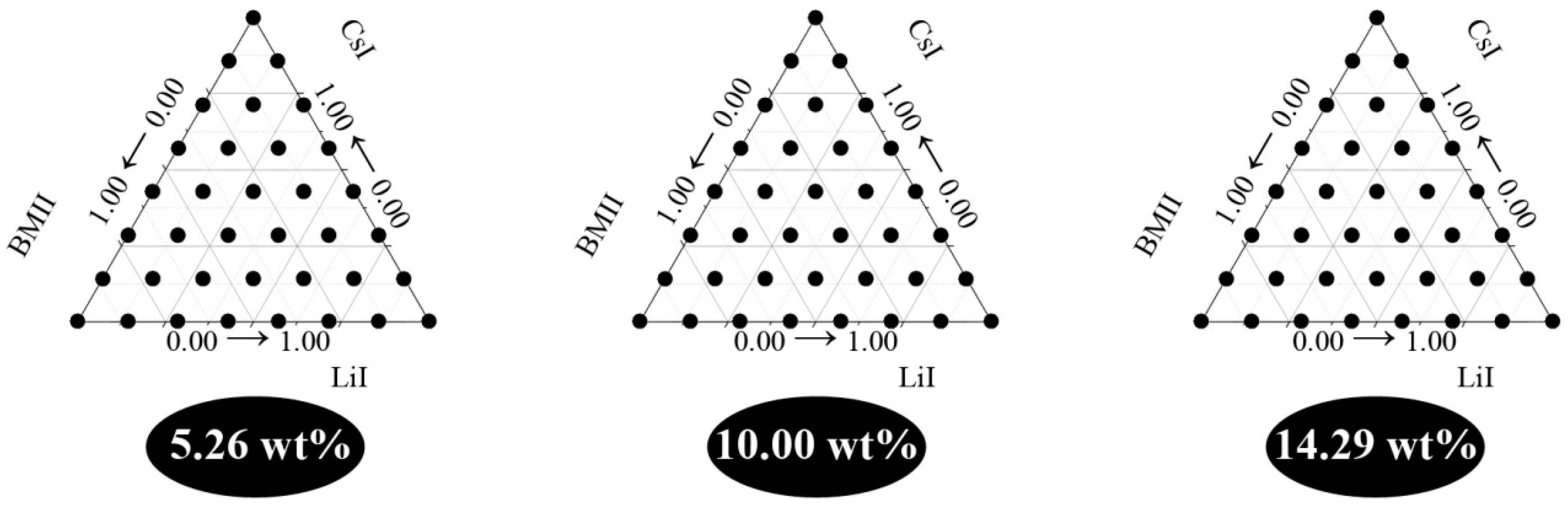
2.1. Sample Preparation

All chemicals in this work were procured from Sigma Aldrich (St. Louis, MO, USA) and used as received without further purification. The synthesis procedure for the phthaloylation of chitosan was similar to that of [31]. Chitosan (viscosity > 400 mPa·s, 1% in acetic acid at 20 °C) and excess phthalic anhydride were refluxed at 110 ± 10 °C under nitrogen atmosphere for 6 h in dimethylformamide (DMF). The reaction was allowed to proceed for another 20 h at a reduced temperature of 60 °C after which the mixture became a clear yellow viscous solution. The precipitate obtained by pouring the solution into ice-water was collected by filtration, and then further purified by redissolving in DMF and reprecipitation in ethanol. The product, phthaloyl chitosan (PhCh) was dried in vacuum at 60 °C until constant weight. Purity of the samples was validated by 1H NMR, δ (ppm, DMSO, 400 MHz): 7.26–8.14 (m, 4H, aromatic–H), 2.00–5.00 (m, 9H, backbone aliphatic–H).
The synthesis procedure for the ionic liquid of 1-butyl-3-methylimidazolium iodide (BMII) was done by reacting equimolar amounts of 1-methylimidazole and 1-iodobutane dissolved in cyclohexane at 70 °C under nitrogen blanket for 24 h. The resultant product was washed with n-hexane to remove the unreacted material. The product was dried in vacuum at 60 °C until constant weight. Purity of the samples was validated by 1H NMR, δ (ppm, CDCl3, 400 MHz): 9.89 (s, 1H, –NCH=N+–), 7.52 (dd, 2H, –N–CH=CH–N+–), 4.32 (t, 2H, –CH2–N–), 4.10 (s, 3H, =N–CH3), 1.90 (m, 2H, –CH2–CH2–CH2–), 1.37 (m, 2H, –CH2–CH2–CH3), 0.95 (t, 3H, –CH2–CH2–CH3).
The gel polymer electrolyte (GPE) was prepared by stirring well 0.4 g of ethylene carbonate (EC), 0.4 g of DMF, and w g of salt system where w is the sum of predetermined amounts of lithium iodide (LiI), caesium iodide (CsI), and BMII. Subsequently, 0.1 g of PhCh was added into the salt solution. This mixture was vigorously stirred and heated to 60 °C and the procedure was halted when it became a homogeneous gel. After cooling to room temperature, iodine (10% of w) was added and stirred until a homogeneous GPE was obtained.
Preliminary runs for the GPE preparation were done with w values in increments of 0.05 g from 0.00 g (0.00 wt %) to 0.40 g (30.77 wt %) using a salt system of LiI:CsI:BMII in a ratio of 0.33:0.33:0.33. However, it was found that the system was only miscible up to 0.15 g (14.29 wt %) salt content. Therefore, to analyze the effects of the independent variables simultaneously, the design of experiment (DoE) employed consisted of process variables (in this work, three levels were used corresponding to 5.26 wt %, 10.00 wt %, and 14.29 wt %) and mixture variables. As shown in Figure 2, for each level, 36 samples were prepared. Samples located on the vertex of the ternary diagram represent a single component system, those on the edges are binary mixtures and any sample points inside the ternary diagram are ternary mixtures). The sequence of experimental preparation and measurement runs were randomized to minimize bias in the readings obtained.
Figure 2. Design of experiment for the preparation of the PhCh–(LiI:CsI:BMII) GPE.
Polymers 08 00022 g002

2.2. General Characterization

1H NMR measurements were performed with an ECA 400 MHz spectrometer (JEOL, Tokyo, Japan). Attenuated Total Reflectance-Fourier Transform Infrared (ATR-FTIR) spectra were recorded with a Spotlight 400 spectrometer (PerkinElmer, Beaconsfield, Bucks, UK). The acquisition parameters were done with a total of 128 accumulations at 2 cm−1 resolution with a spectral range from 4000–600 cm−1.

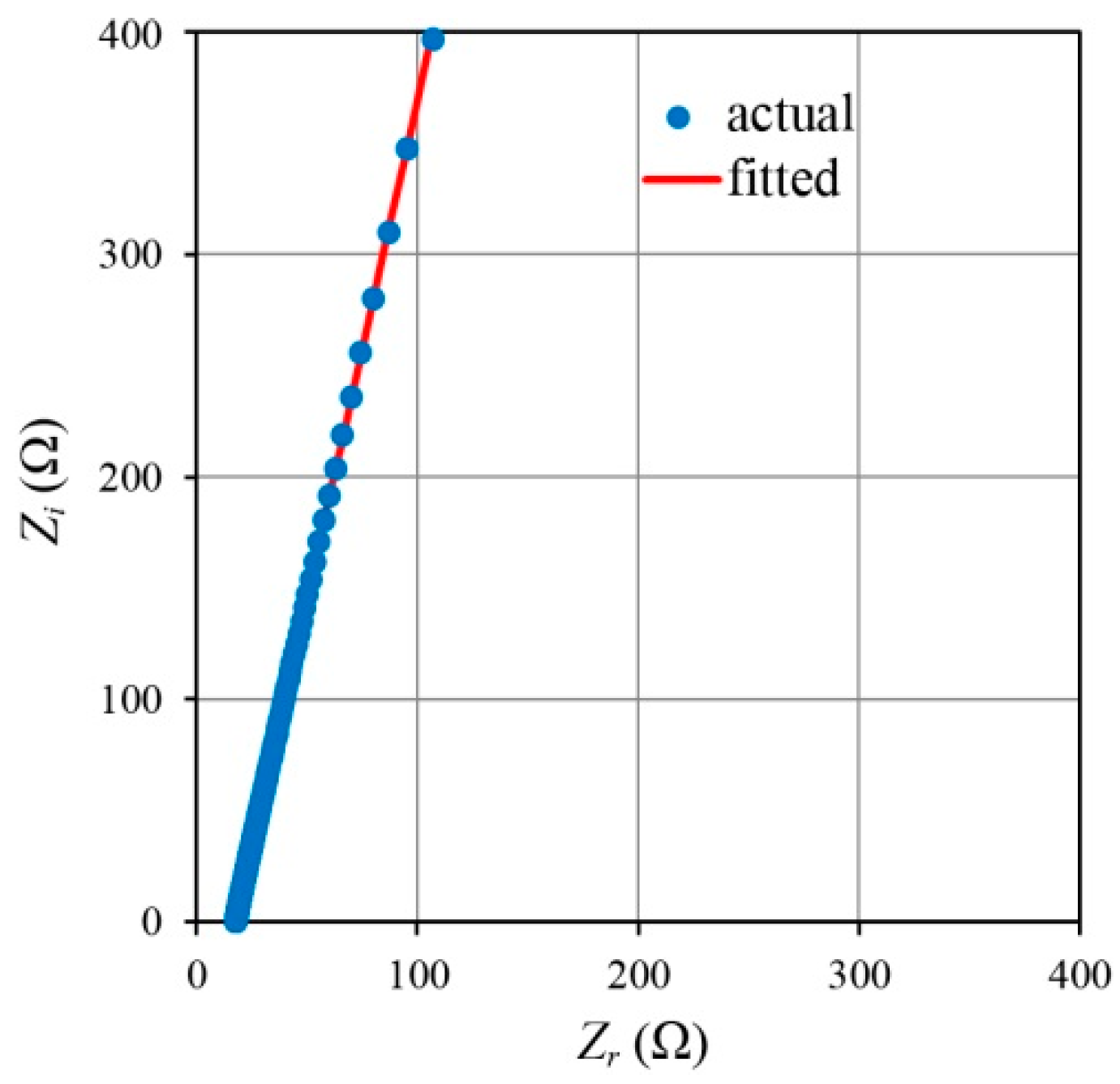
2.3. Electrochemical Impedance Spectroscopy (EIS)

Electrochemical impedance spectroscopy (EIS) measurements were done using an IM3590 instrument (HIOKI, Nagano, Japan) from 50 Hz to 200 kHz with an average of three replicate readings at each experimental point. A sample cell holder with two stainless steel disc electrodes 1 cm in diameter was used to sandwich the GPE with a thickness of 0.13 cm. The impedance data was processed in a complex impedance plot where the imaginary part Zi was plotted against its real part Zr. Nyquist plots generated by impedance measurements can normally consist of (i) a depressed semicircle; (ii) a tilted spike or (iii) a depressed semicircle with a tilted spike. All the results in this work however, showed a Nyquist plot behavior with only a tilted spike as shown in Figure 3.
Figure 3. Typical Nyquist plot for the PhCh–(LiI:CsI:BMII) GPE.
Polymers 08 00022 g003
The Nyquist plot was fitted (using a non-linear least squares method using Microsoft Excel’s Generalized Reduced Gradient solver algorithm) to an equivalent circuit consisting of a resistor and a constant phase element (CPE) in series to obtain RB, the bulk impedance at the intersection of the plot with the real impedance axis. The real and negative imaginary parts of the Nyquist plot consisting of a tilted spike are given by the equations [32]:
Z r = R B + cos ( π p 2 ) Q ω p
and
Z i = sin ( π p 2 ) Q ω p
where ω is the angular frequency, Q is the capacitance due to the electrical double layer (EDL) formed at the electrode/electrolyte interface during the impedance measurement [33] and p which has a value between 0 and 1 is the skew parameter that controls the degree of inclination of the tilted spike from the Zr axis. Hence, the ionic conductivity of the samples was calculated using the following equation:
σ = 2 d R B A
where d is the half thickness of the sample, and A is the electrode/electrolyte contact area.
Apart from conductivity (σ) values, other PhCh–(LiI:CsI:BMII) GPE electrical properties were also evaluated. Bandara and Mellander [32] have shown that, using only impedance measurements, it is possible to obtain the number density and mobility of charge carriers since in principle, the conductivity is the product of these parameters. Arof et al. [34] have further developed and derived in detail a method based on this to determine the diffusion coefficient (D), ion mobility (μ) and number density of the charge carriers (n). Briefly, the diffusion coefficient (D) was given as:
D = ( Q 1 ε r ε 0 A ) 2 τ 2
where εr is the dielectric constant of the electrolyte, ε0 is the vacuum permittivity (8.85 × 10⁻¹⁴ F·cm−1) and τ 2 is 1 / ω 2 with ω 2 being the angular frequency corresponding to the minimum in the imaginary impedance, Zi. From the impedance data, εr for each sample can be obtained by a plot of the real part of the complex permittivity, εr, versus frequency, f. The impedance data was substituted in the equation below:
ε r = Z i ( Z r 2 + Z i 2 ) ( d ω ε 0 A )
It was observed that all the samples showed a constant value between log f = 4.5 and log f = 5.0. Hence, the value of the dielectric constant, εr, for all the samples was taken at the high frequency of 200 kHz. The mobility (µ) of the charge carriers can then be determined from the Nernst–Einstein relation:
μ = e D k b T
where k b is the Boltzmann constant (1.38 × 10⁻²³ J·K−1), T is the absolute temperature in Kelvin and e is the electron charge (1.602 × 10⁻¹⁹ C). Finally, the number density of charge carriers (n) can be obtained using the following equation:
n = σ μ e

3. Results and Discussion

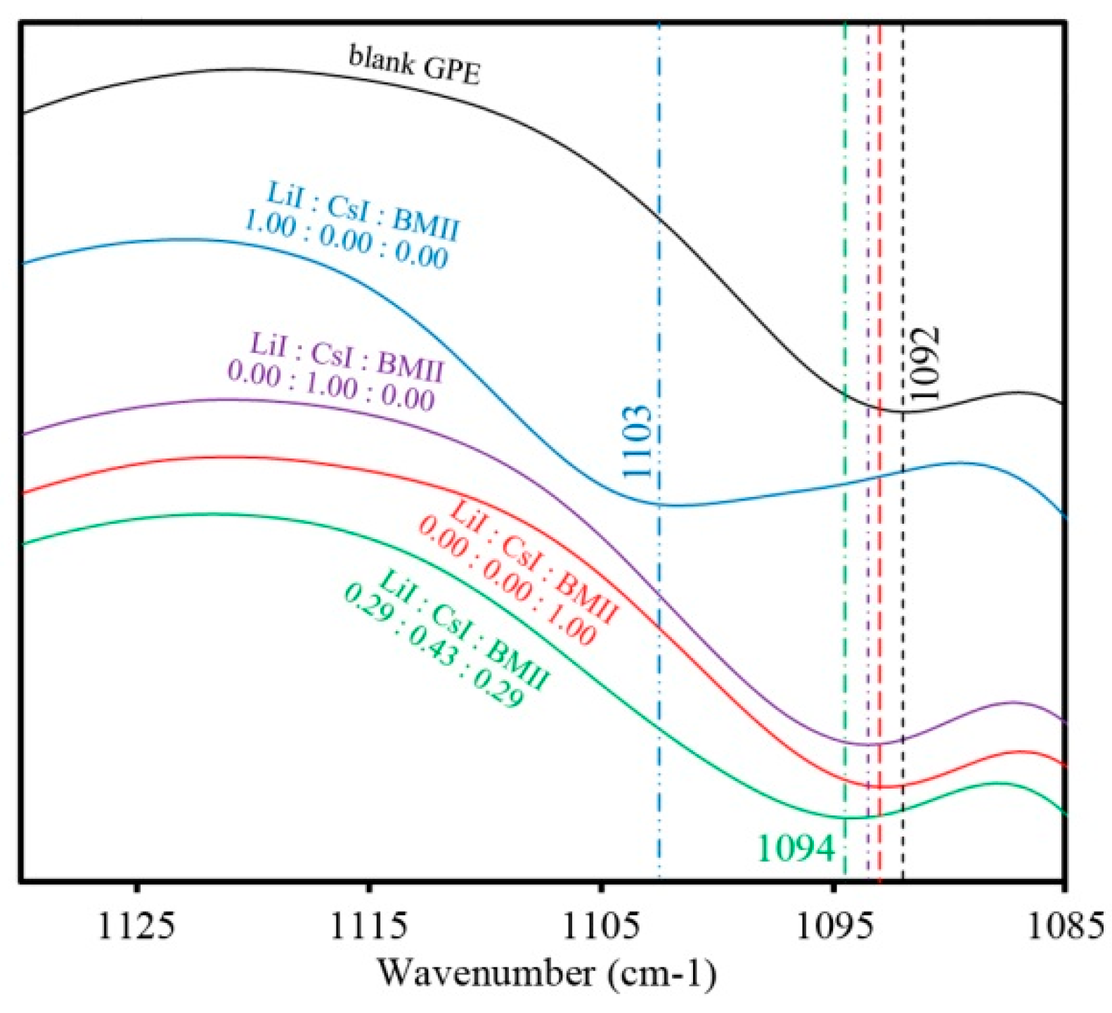
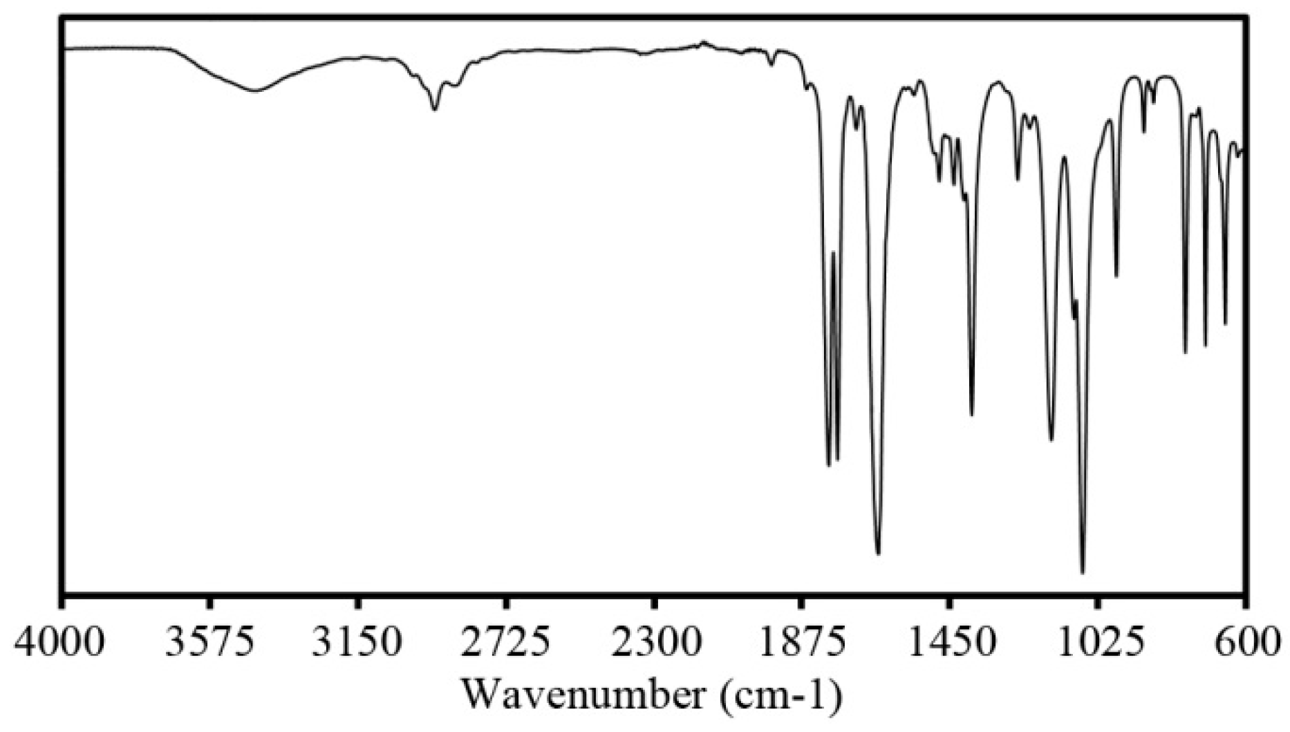
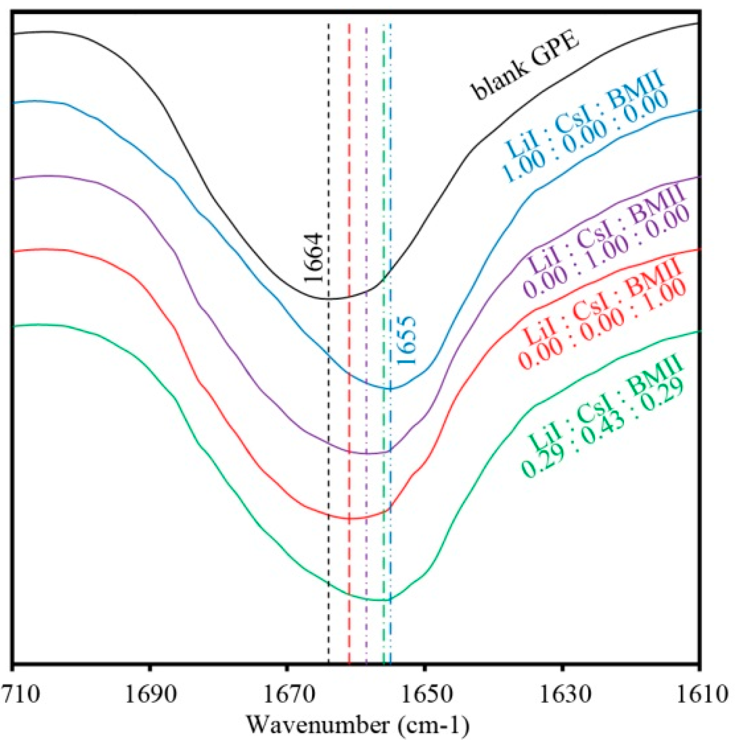
3.1. FTIR Spectra of the PhCh–(LiI:CsI:BMII)

Figure 4 shows the FTIR spectra that is typical of the PhCh–(LiI:CsI:BMII) GPE samples. Peaks attributed to the ether C–O–C group appeared in the range of 1000 to 1120 cm−1. Samples with different salt contents showed a peak that varied in position from 1092 to 1103 cm−1 (Figure 5) implying that there is a coordination of salt ions to the polymer matrix. The peak at 1256 cm−1 is due to C–N asymmetric stretching mode. The intense peak around 1660 cm−1 is attributed to the amide group presence in the GPE. This peak also tends to shift to lower wavenumbers when varying salt contents are added to the system as seen in Figure 6 further confirming coordination interactions of the salts in the polymer [35]. The strong peak at 1773 and 1798 cm−1 is due to carbonyl C=O stretching. The peak at 2930 cm−1 is due to the CH3 symmetric stretching mode. The broad peak in the range of 3200 to 3700 cm−1 corresponds to the O–H and N–H group of the GPE.
Figure 4. FTIR spectra of the PhCh–(LiI:CsI:BMII) GPE.
Polymers 08 00022 g004
Figure 5. FTIR spectra of selected PhCh–(LiI:CsI:BMII) GPE samples for the ether absorption bands ranging from 1085 to 1130 cm−1.
Polymers 08 00022 g005
Figure 6. FTIR spectra of selected PhCh–(LiI:CsI:BMII) GPE samples for the amide absorption bands ranging from 1610 to 1710 cm−1.
Polymers 08 00022 g006

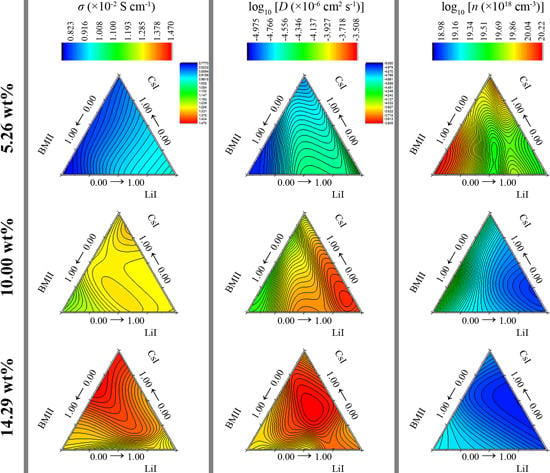
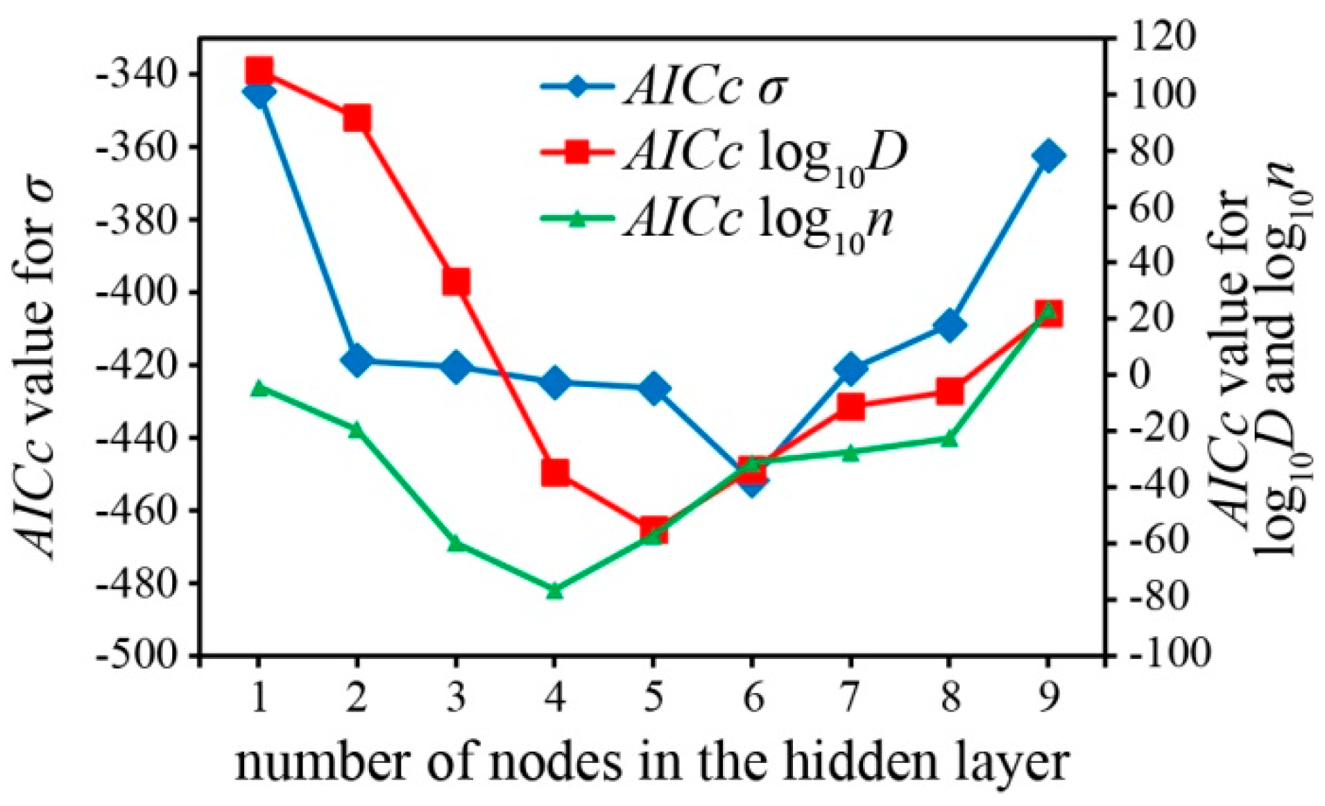
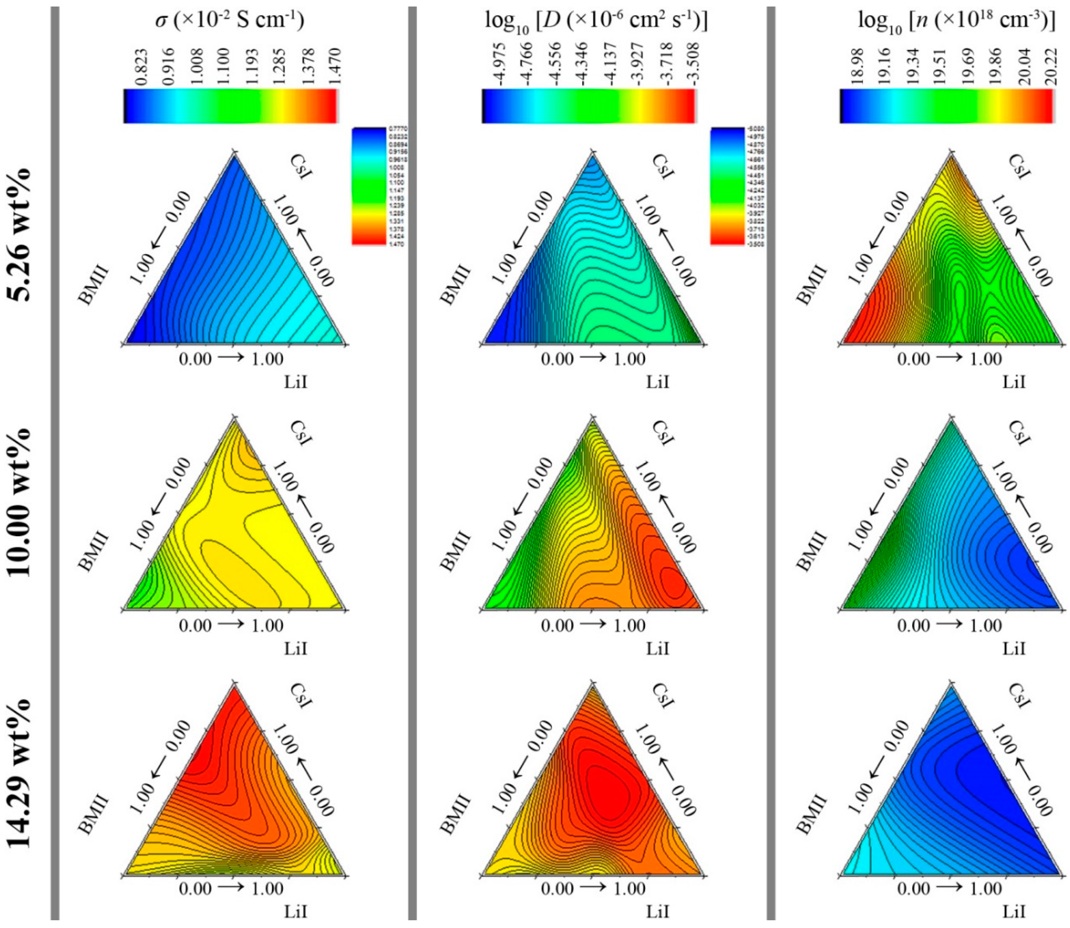
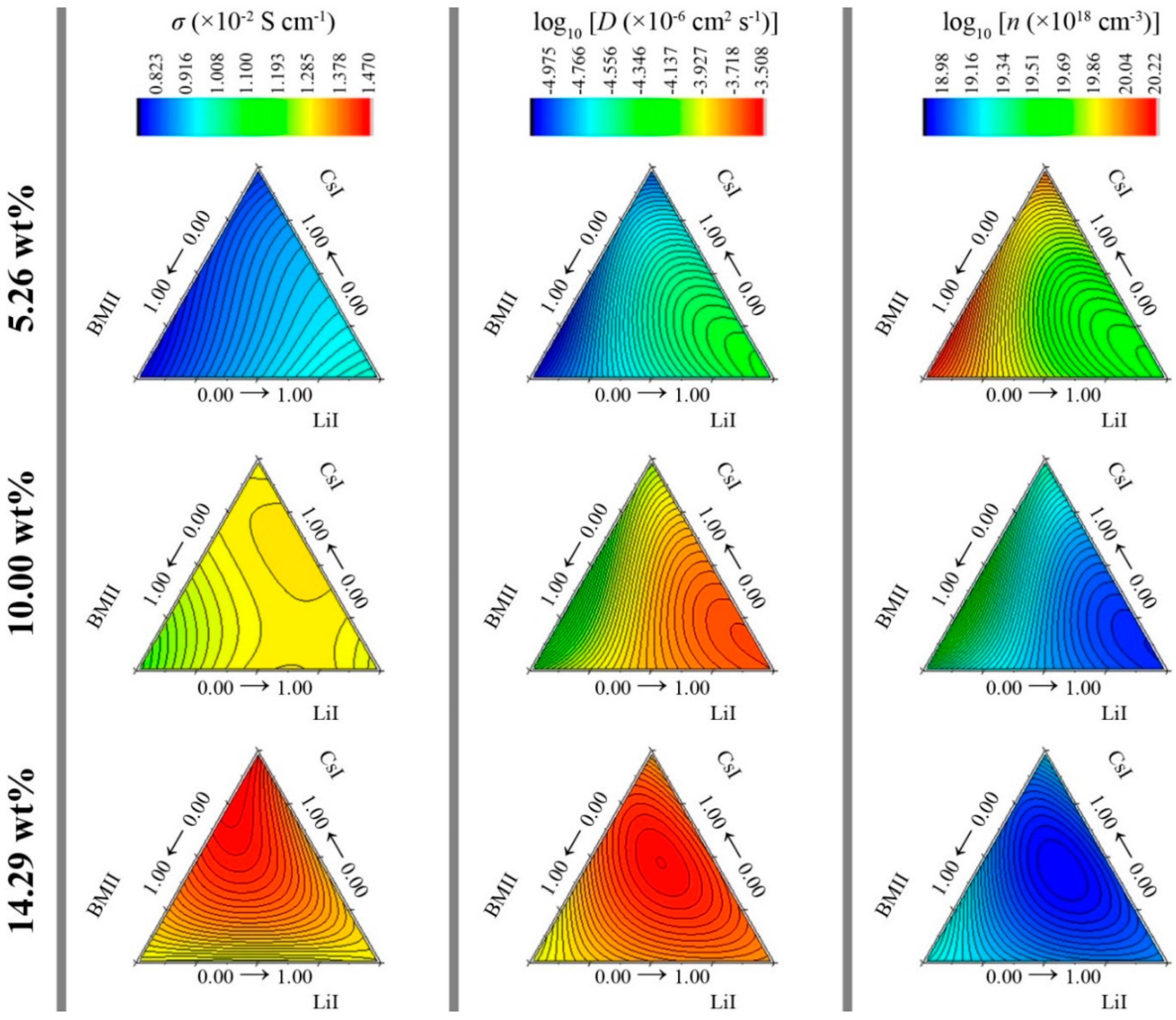
3.2. Surface Modeling

The effects of the four different input variables on the responses of conductivity (σ), diffusion coefficient (D), and number density of charge carriers (n) were studied. The first, second, and third variable is the mixture ratio of LiI, CsI, and BMII, respectively, in the GPE system. The fourth variable is the sum wt % of the salt system. Table 1 shows the complete experimental design of the factor combinations, together with the experimental response outputs. Experimentally, the highest conductivity was obtained for the sample with LiI:CsI:BMII in ratio of 0.00:0.71:0.29 at 14.29 wt % with σ = 1.495 × 10⁻² S·cm−1.
Table 1. DoE for the independent variables used in this study along with the observed response.
σ (×10−2 S·cm−1)D (×10−6 cm2·s−1)n (×1018 cm−3)
LiI ratioCsI ratioBMII ratio5.26 wt %10.00 wt %14.29 wt %5.26 wt %10.00 wt %14.29 wt %5.26 wt %10.00 wt %14.29 wt %
0.430.570.000.9131.3131.33234.83180.40185.2442.2511.7111.57
0.430.430.140.8981.2491.37414.79118.45348.4898.0617.046.35
0.430.290.290.9061.3141.43937.90142.42306.0538.5914.877.59
0.570.430.000.9121.3071.32649.96301.30285.2029.386.987.58
0.570.290.140.9171.2901.38625.43204.88302.3658.0110.147.79
0.570.140.290.9671.2781.37150.76297.61200.6530.736.9111.06
0.710.290.000.9381.2951.34839.03168.79181.4738.6612.7112.36
0.710.140.140.9401.2881.33824.12214.20233.3762.759.689.28
0.710.000.290.9351.3481.29521.09246.71221.5571.658.859.65
0.860.140.000.9871.2891.30759.82242.16194.7826.558.5810.95
0.860.000.140.9721.2781.28935.05228.26169.6844.699.0112.62
1.000.000.000.9851.2641.27048.09198.48222.7533.1710.259.18
0.290.290.430.8831.2981.41523.23214.89365.0661.499.726.29
0.290.430.290.8311.3171.42416.27190.98370.3082.1311.136.48
0.140.430.430.8741.2961.44817.3793.58265.6780.9322.309.10
0.140.570.290.8511.2981.45234.8088.54382.4439.3723.846.33
0.000.570.430.8251.2771.45520.2099.26140.1465.7320.7117.21
0.290.570.140.9121.2951.40345.18168.66266.2232.5612.398.92
0.290.710.000.8791.3391.38015.35153.54219.2392.2414.0610.33
0.000.710.290.7941.2921.4957.7671.91356.08164.9128.936.80
0.140.710.140.8351.2971.44514.07110.76155.1895.6018.8715.03
0.140.860.000.8591.3121.42413.31150.49241.17103.9614.039.76
0.000.860.140.8471.2771.46629.3666.24256.9947.8031.129.22
0.001.000.000.8061.2801.43310.6795.69118.54121.4621.5319.71
0.430.140.430.8891.2761.36353.7982.04156.3626.6025.0914.36
0.570.000.430.9331.3141.24831.63197.06113.0047.5110.9917.78
0.000.430.570.8361.2691.40613.6350.09136.3698.6740.8716.61
0.140.290.570.8281.3261.36414.27114.07146.8593.4618.7315.76
0.290.140.570.8791.2671.35121.73199.37159.2965.2310.0014.06
0.430.000.570.9261.2931.24037.34159.30155.0739.9613.0612.89
0.000.290.710.7591.2221.3454.5132.77141.64270.9660.0515.80
0.140.140.710.8311.2581.33614.1279.94180.5894.6825.3411.90
0.290.000.710.8231.2391.23415.92100.72125.9583.3219.8215.78
0.000.140.860.7791.1881.31811.8848.46128.09105.6239.8516.57
0.140.000.860.8151.2291.3148.8996.66131.55148.5820.5316.49
0.000.001.000.7851.2131.2817.6466.66148.05165.3229.3114.12
The analysis, evaluation and estimation of the accuracy and applicability for the polynomial models were determined with Design Expert® Software Version 6.0.6. In the data preprocessing step, all the input variables in Table 1 (for x 1 , x 2 ,   x 3 , and x 4 representing LiI, CsI, BMII ratios and the sum wt % of the salt system, respectively) were normalized into dimensionless values according to the equation below:
X new = a + ( X old X min ) ( b a ) ( X max X min )
where x i ( a ; b )
  • X new 
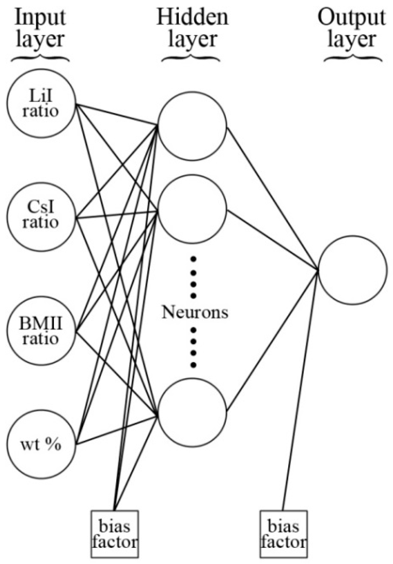
is the normalized input variable;
  • a is the new minimum value of the normalized input variable;
    b is the new maximum value of the normalized input variable;
  • X old is the original input variable;
  • X min is the minimum value of the original input variable;
  • X max is the maximum value of the original input variable.
For the RSM procedure in this work, a = 0 and   b = 1 for the mixture variables and a = 1 and   b = 1 for the process variable. The response outputs can then be evaluated with the different types of response surface models (i.e., linear, two-factor interaction (2FI), quadratic, reduced cubic, and full cubic) to compare the appropriateness of each model. The response surface models consist of polynomials with coefficients and would take the general form as follows:
y ( x , w ) = w 0 + i = 1 D w i x i + i = 1 D j = 1 D w i j x i x j + i = 1 D j = 1 D k = 1 D w i j k x i x j x k +
(not all of the coefficients are independent due to interchange symmetries amongst the x variables). In practice, to capture complex dependencies in the data, a higher-order polynomial may need to be used. The coefficient of determination R2 indicates how well the data fits a statistical model where a good fit will have values close to 1. The use of an adjusted R2 takes into account the phenomenon of the R2 spuriously increasing when additional terms are added to the RSM model and its value is ≤R2. Unlike R2, the adjusted R2 increases when a new term is added only if the new term improves the R2 more than would be expected by chance.
The analysis of variance (ANOVA) done on each of the response data revealed that there were model terms with Prob > F values that were greater than 0.1 indicating that their contribution to the model was not significant. To improve the model fit, a backward regression procedure was performed from the full cubic model. The unnecessary terms which had high Prob > F values were removed stepwise. From this procedure, it was found that all the RSM for conductivity (σ), diffusion coefficient (D), and number density of charge carriers (n) followed a crossed reduced cubic × quadratic model (corresponding to the crossed DoE for mixture variable × process variable). The ANOVA also revealed that in the case of D and n which had a high max to min response ratio, a power transform to the data set was required to stabilize the variance and make the data more normal distribution-like. A Box-Cox plot was used to determine the suitable power transform and it was recommended as follows [36]:
y = log 10 y
where y’ is the transformed response and y is the original response.
Table 2 lists the outcomes for the optimized models for each of the responses. The signal to noise (S/N) ratio compares the range of the predicted values at the design points to the average prediction error and typically, ratios greater than 4 indicates adequate model discrimination [37]. In this case, all the S/N ratio values are well above 4; therefore, the design space can be navigated by the selected model. These models can be used to predict the response values within the limits of the experiment. The final equation for the developed models in Table 2 in terms of coded (normalized) factors is as follows:
σ (×10−2 S·cm−1) = 1.267 x1 + 1.256 x2 + 1.180 x3 + 0.144 x1x2 + 0.276 x1x3 + 0.157 x1x4 + 0.162 x2x3 + 0.315 x2x4 + 0.251 x3x4 − 0.129 x1x42 − 0.120 x2x42 − 0.154 x3x42 − 0.449 x1x2x3 − 0.089 x1x2x4 − 0.113 x1x3x4 + 0.096 x2x3x4 − 0.198 x1x2(x1-x2) + 0.125 x2x3(x2-x3) − 0.180 x1x2x42 − 0.249 x1x3x42 − 0.009 x2x3x42 + 1.034 x1x2x3x4 + 1.482 x1x2x3x42 + 0.287 x1x2x42(x1-x2)
log10 [D (×10−6 cm2·s−1)] = −3.648 x1 − 4.085 x2 − 4.161 x3 + 0.535 x1x2 + 0.370 x1x3 + 0.294 x1x4 − 0.620 x2x3 + 0.583 x2x4 + 0.547 x3x4 − 0.403 x1x42 − 0.300 x2x42 − 0.349 x3x42 + 2.933 x1x2x3 + 0.153 x2x3x4 + 1.094 x2x3(x2-x3) + 1.136 x2x3x42
log10 [n (×1018 cm−3)] = 18.961 x1 + 19.396 x2 + 19.447 x3 − 0.518 x1x2 − 0.325 x1x3 − 0.236 x1x4 + 0.628 x2x3 − 0.461 x2x4 − 0.444 x3x4 + 0.351 x1x42 + 0.232 x2x42 + 0.267 x3x42 − 2.722 x1x2x3 − 0.079 x2x3x4 − 1.045 x2x3(x2-x3) − 1.059 x2x3x42
Table 2. Optimized models for each of the response properties.
ResponseRSM R2RSM Adjusted R2S/N Ratio4-h-1 ANN R2
Conductivity, σ(×10−2 S·cm−1)0.99190.989765.140.9936
log10 Diffusion coefficient, log10 [D (×10−6 cm2·s−1)]0.92180.909128.070.9317
log10 number density of charge carriers, log10 [n (×1018 cm−3)]0.89200.874323.910.8989
The RSM models are graphically represented in Figure 7. It can be seen that as the sum wt % of the salt system increases from 5.26 to 14.29 wt %, the conductivity increases. The position for the mixture ratio combination of LiI, CsI, and BMII that led to the highest conductivity varies for each level. At 5.26 wt %, the σ was highest when LiI ratio was the highest. As the sum wt % of the salt system increased further, the highest σ for each level shifted along the ridge of the LiI-CsI region and at 14.29 wt %, the ratio of LiI:CsI:BMII was 0.01:0.81:0.18 showed highest σ at 1.467 × 10⁻² S·cm−1. Since the conductivity is the product of the ionic mobility and number density, it can be inferred from Figure 7 that the contribution towards conductivity was mainly due to the high diffusion of the free ions in the GPE rather than the number density of the charge carriers. The n values decrease as the concentration of the salt system increases.
Figure 7. Plot of predicted RSM for σ (×10−2 S·cm−1), log10 [D (×10−6 cm2·s−1)], and log10 [n (×1018 cm−3)] at various salt concentration levels.
Polymers 08 00022 g007
The normal probability plots in Figure 8 show that the residuals generally fall on a straight line implying that the errors are distributed normally for σ, log10 D, and log10 n. Figure 9 shows that the scatter plot across the graphs does not exceed the threshold of the outlier t. These graphical diagnostic checks imply that the models that have been developed do not violate the independence or constant variance assumption.
Figure 8. Normal probability plot of residuals for (a) σ (×10−2 S·cm−1); (b) log10 [D (×10−6 cm2·s−1)]; and (c) log10 [n (×1018 cm−3)].
Polymers 08 00022 g008
Figure 9. Outlier t plot for (a) σ (×10−2 S·cm−1); (b) log10 [D (×10−6 cm2·s−1)]; and (c) log10 [n (×1018 cm−3)].
Polymers 08 00022 g009
An ANN-based model was also developed during the present study as an alternative to the polynomial RSM, which provides the modeling of complex nonlinear relationships for describing the response for σ, log10 D, and log10 n. ANN, inspired by the structural and/or functional aspect of a biological neural network, has attracted increasing attention in recent years, particularly for process modeling [20,23,24,25,26]. It consists of an input layer (independent variables), a number of hidden layers and an output layer (dependent variables). Each of these layers consists of a number of inter-connected processing units called neurons. These neurons are linked to one another along weighted connections which are passed into the hidden layer. The hidden layer then does all the data processing and produces an output based on the sum of the weighted values from the input layer modified by a sigmoid transfer function. In this study, a hyperbolic tangent-sigmoid transfer function was applied:
f ( x ) = 1 + 2 ( 1 + e 2 x )
The Levenberg–Marquardt back-propagation algorithm was used for network training. The same input and output factors that was used in the RSM approach was fed into the ANN model. In order to achieve fast convergence to the minimal mean square error (MSE), the inputs and outputs were scaled within the uniform range of a = −1 to b = 1 by following Equation (1) to ensure uniform attention during the training process. The Neural Network Toolbox of MATLAB Version 7.12 (R2011a) was used in all ANN calculations. The general scheme of the neural network is shown in Figure 10.
Figure 10. General scheme of the artificial neural network.
Polymers 08 00022 g010
Designing the topology of the network became the first step for training the neural network. For simplicity, each network was developed to represent only one type of response (from Table 1) at a time. Therefore, the topology of the ANN developed was designated as 4-h-1 i.e., four input neurons representing the four variables for the preparation of the PhCh–(LiI:CsI:BMII) GPE, h represents the number of hidden neurons in a single hidden layer, and one output neuron representing one type of response. Using the experimental data, the ANN topologies were built, trained, tested, and validated with a number of hidden layers varying from 1 to 9. The training process was run by a trial and error search method until an optimum model was found and the minimum of mean square error was reached in the validation process.
Similar to the case of developing RSM models, over-fitting of the model could occur when an excessive number of hidden neurons are used. Furthermore, it has been pointed out previously [38,39] that the conventional use of the R2 or adjusted R2 is not a sufficient measure for the goodness of fit in nonlinear models. To supplement this deficiency, we used the Akaike Information Criterion (AIC) [40,41,42], a model selection method that is widely accepted for measuring the validity within a cohort of nonlinear models [43]:
A I C = 2 p 2 ln ( L )
where p = number of parameters and ln(L) = maximum log-likelihood of the estimated model. The latter, in the case of a nonlinear fit with normally distributed errors, is calculated by:
ln ( L ) = 0.5 × ( N × ( ln 2 π + 1 ln N + ln i = 1 n r i 2 ) )
with r1, ..., rn = the residuals from the nonlinear least-squares fit and N = their number. For small sample sizes, the bias-corrected AIC variant is given as (AICc):
A I C c = A I C + 2 p ( p + 1 ) n size p 1
where nsize is the sample size. Operationally, the best model is selected from the smallest AICc value computed for each of the 4-h-1 models. The calculated AICc values for the ANN networks of the response outputs are shown in Figure 11, and in all cases it was observed that the number of hidden nodes that would be sufficient to build the topology of the neural network without over-fitting for the models of σ, log10 D, and log10 n were six, five, and four, respectively. The ANN models are graphically represented in Figure 12. Although the contour shapes of the ANN appears to be comparable to the RSM, the R2 calculated from the developed 4-h-1 ANN models as shown in Table 2, indicate that the the 4-h-1 ANN models have a better fit over the RSM models. The ANN model showed highest σ at 1.467 × 10⁻² S·cm−1 from a LiI:CsI:BMII ratio of 0.01:0.63:0.36 at 14.29 wt %.
Figure 11. AICc for all the response outputs.
Polymers 08 00022 g011
Figure 12. Plot of predicted ANN for σ (×10−2 S·cm−1), log10 [D (×10−6 cm2·s−1)], and log10 [n (×1018 cm−3)] at various salt concentration levels.
Polymers 08 00022 g012

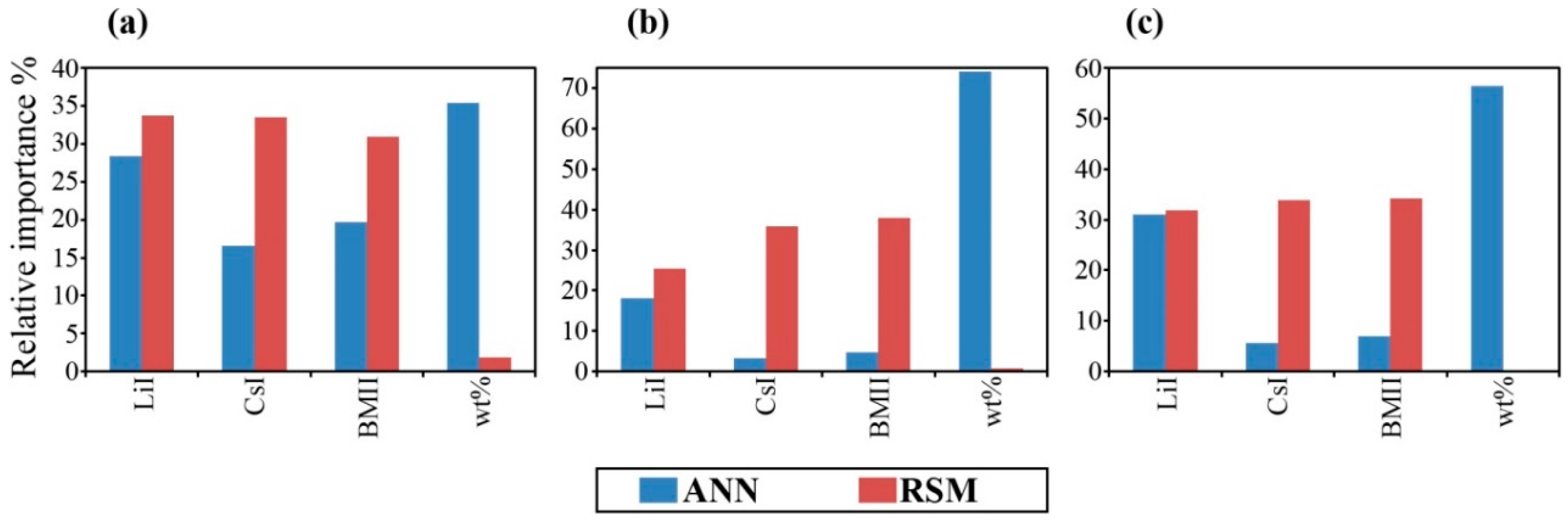
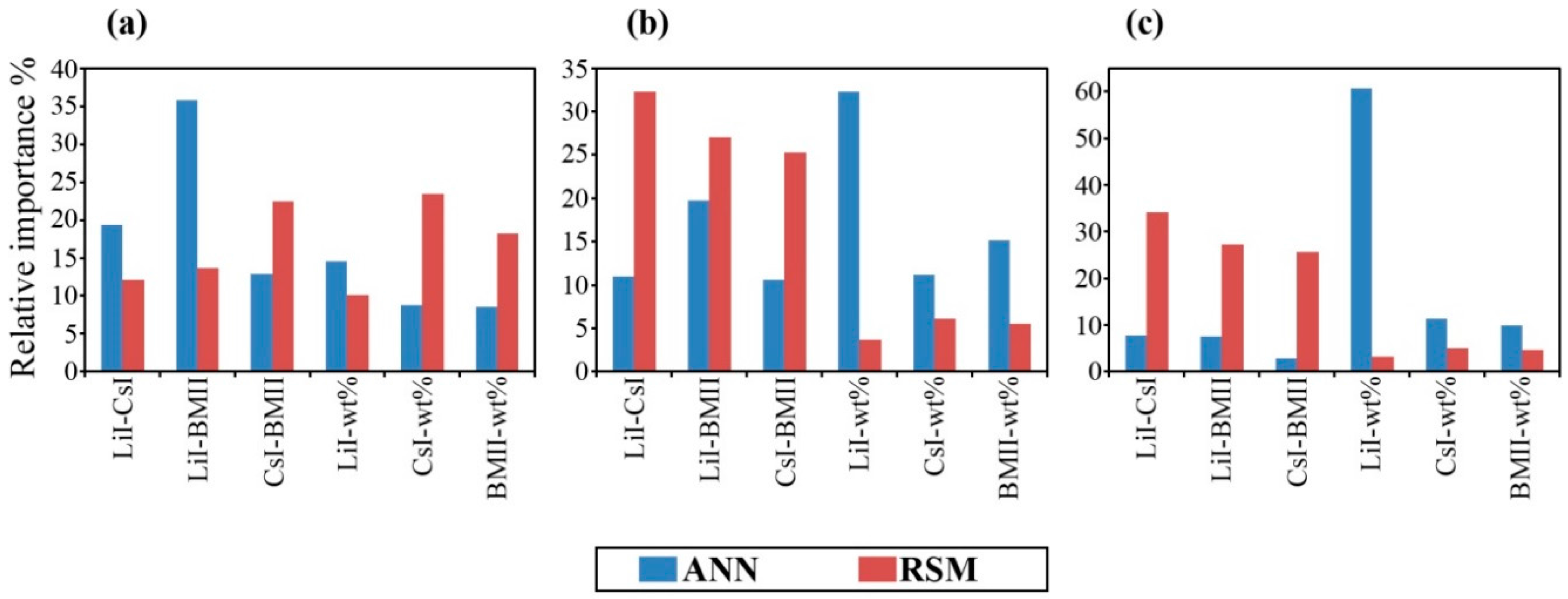
3.3. Determination of the Importance of Each Input Variable

Once the response models have been developed, it would be of interest to determine which of the four input variables (mixture ratio of LiI, CsI, BMII, and the sum wt % of the salt system) would influence the properties of the prepared PhCh–(LiI:CsI:BMII) GPE the most. The fit of the RSM models are limited by the fact that it is constrained to have a polynomial shape, whereas the ANN surface model has the advantage that it can accommodate non-linear shapes. Typically, the importance of each input variable in RSM models can be evaluated quite simply by the weight coefficients where positive values indicate that the corresponding input would increase the value of the response output and vice versa. The F-value can also be used where the larger its magnitude for the corresponding coefficient terms, the more significant is the contribution of the corresponding coefficient term [44]. However, the weight coefficients in the ANN models cannot be used directly in a similar manner with the RSM methods. Many researchers that adopted the ANN approach have also labeled it as a “black box” because they provide little explanatory insight into the relative influence of the independent variables in the prediction process [45,46,47,48]. There should still be some other way to extract information about the relative importance that the input variables have on the output since the ANN can be regarded as analogous to real biological neurons, where each weight influences the proportion of the incoming signal that will be transmitted into the neuron’s body.
One method adopted for the determination of relative contribution of input factors was by using the partial derivatives (PaD) [49]. The sensitivity of network outputs according to small input perturbations is represented by the Jacobian matrix dy/dxt = [∂y/∂x]m×n, which links the modification of inputs, xj, and the variation of outputs, yj = f(xj) . For a network with n inputs, one hidden layer with ni nodes, and one output (i.e., m = 1), the gradient vector of yj with respect to xj when a hyperbolic tangent sigmoid function is used for the activation is dj = [dj1,…,dje,…,djn ]T, with:
d je = s j h = 1 n h w e h w h o ( 1 I h j 2 )
where sj = (1 − f(x)2) is the derivative of the output node with respect to its input, Ihj is the output of the hth hidden node for the input xj, the scalars weh and who are the weights between the eth input node and the hth hidden node, and between the hth hidden node and the output node. The partial derivatives can then be interpretable, but it has to be evaluated at a large, representative sample of points from the input space. Due to the small experimental dataset (36 samples × 3 levels), a larger dataset consisting of 4851 points (231 samples × 21 levels) was randomly generated within the input space to obtain information representative of the developed models. The next step was to summarize this large collection of numbers to a single measure of importance for each input to report an average value. This was done by the sum of the square partial derivatives obtained per input variable:
S S D i = j = 1 N ( d j i 2 )
The calculated relative importance of the input variables is shown in Table 3 and Figure 13. A similar treatment was adopted for the RSM models using PaD for comparison. RSM PaD generally showed little sensitivity for mixture variables whereas ANN PaD showed distinctly that LiI had the highest contribution and although CsI and BMII contribution was similar, CsI had the lowest contribution. This is possibly due to Li+ being the smallest cation, which would have greater mobility in the system. The ANN PaD showed reasonably that the process variable for the sum wt % of the salt system had significant contribution to the response properties compared to the RSM PaD which showed negligible effect.
Table 3. PaD relative importance of individual input towards the output response properties of (a) σ (×10−2 S·cm−1); (b) log10 [D (×10−6 cm2·s−1)]; (c) log10 [n (×1018 cm−3)] in terms of percentages.
Variableσ (×10−2 S·cm−1)log10 [D (×10−6 cm2·s−1)]log10 [n (×1018 cm−3)]
ANN PaD%RSM PaD%ANN PaD%RSM PaD%ANN PaD%RSM PaD%
x1, LiI28.4033.7318.0425.3531.0131.83
x2, CsI16.5233.503.2235.885.5733.91
x3, BMII19.6830.914.8137.947.0434.24
x4, wt %35.391.8573.940.8456.380.02
Figure 13. PaD relative importance% of single input factors towards the output response properties of (a) σ (×10−2 S·cm−1); (b) log10 [D (×10−6 cm2·s−1)]; and (c) log10 [n (×1018 cm−3)].
Polymers 08 00022 g013
Furthermore, to analyze the contribution of all possible two-way interactions of input variables a similar method to the modification (PaD2) proposed by [50] was used:
d j 12 = ( 1 f ( x ) 2 ) [ ( 2 f ( x ) ) h = 1 n h w 1 h w h o ( 1 I h j 2 ) h = 1 n h w 2 h w h o ( 1 I h j 2 ) + h = 1 n h w 1 h w 2 h w h o ( 2 I h j ) ( 1 I h j 2 ) ]
where w1h and w2h are, respectively, the weights between the first studied input neuron and the hth hidden neuron, and between the second studied neuron and the hth hidden neuron.
Although the shape of the contour fit in the RSM was comparable to the ANN model, it appears that the ANN has a slightly different approach for the interpretation of the contribution of two way interactions compared to the RSM (Table 4 and Figure 14). This result is not unexpected since the ANN model is not hindered by the polynomial constraints of the RSM model. The better fit of the ANN gives a hint on the salt-salt compatibility where LiI-BMII was the highest contributor compared to CsI-BMII in RSM. The ANN PaD2 also showed that the individual salt concentration contribution was highest with LiI but CsI for RSM. It would seem that the RSM PaD and PaD2 tends to favor CsI contribution since the electrical properties in the fitted ternary contours showed it was highest along the ridge of the LiI–CsI region. On the other hand, ANN PaD and PaD2 showed that the contribution was favored from LiI even though the ternary contours showed the best properties near the CsI region (at the highest salt concentration of 14.29 wt %). This should not be construed as counterintuitive however, since as described earlier in the preliminary runs for the GPE preparation, it was observed that the salt system was no longer miscible at salt concentrations above 14.29 wt %. Although the LiI-CsI-BMII salt system in the GPE would behave synergistically to give the best conductivity near the CsI region, this is only true at the concentration level of 14.29 wt %. It is possible that at much higher concentrations, the compatibility of CsI with LiI and BMII could hinder its solubility in the salt system. Thus, it has been shown the better predictive power that ANN has over the RSM approach.
Table 4. PaD2 relative importance of two-way interactions towards the output response properties of (a) σ (×10−2 S·cm−1), (b) log10 [D (×10−6 cm2·s−1)], and (c) log10 [n (×1018 cm−3)] in terms of percentages.
Variableσ(×10−2 S·cm−1)log10 [D (×10−6 cm2·s−1)]log10 [n (×1018 cm−3)]
ANN PaD2%RSM PaD2%ANN PaD2%RSM PaD2%ANN PaD2%RSM PaD2%
x1x2, LiI-CsI19.3012.0811.0132.347.7534.18
x1x3, LiI-BMII35.7813.7119.7827.047.4927.28
x2x3, CsI-BMII12.9222.4410.6325.332.8825.73
x1x4, LiI-wt %14.6010.1532.253.7160.623.23
x2x4, CsI-wt %8.8223.4411.206.0811.284.97
x3x4, BMII-wt %8.5818.1815.145.509.984.61
Figure 14. PaD2 relative importance% of two-way interactions towards the output response properties of (a) σ (×10−2 S·cm−1); (b) log10 [D (×10−6 cm2·s−1)]; (c) log10 [n (×1018 cm−3)].
Polymers 08 00022 g014

4. Conclusions

The preparation of a gel polymer electrolyte system based on phthaloylchitosan was successfully prepared using lithium iodide, caesium iodide, and 1-butyl-3-methylimidazolium iodide as the mixed salt system. From the EIS analyses, it was found that the range of conductivities obtained experimentally was from 0.759 × 10⁻² to 1.495 × 10⁻² S·cm−1. The ANN model showed better predictive capabilities compared to the RSM approach. The highest conductivities were obtained in the ternary region near CsI at 14.29 wt %. However, relationship studies of the contributing input factors showed that LiI has the highest compability in the mixed salt system.

Supplementary Materials

The following are available online at www.mdpi.com/2073-4360/8/2/22/s1. Figure S1. (a) Appearance typical of the GPE prior to adding iodine. Note that the gel is capable of holding the magnetic stirring bit in place without falling to the bottom; and (b) appearance typical of the GPE after adding iodine. Note that the gel appears to be covering the entire length of the vial because the vial was tilted horizontally during stirring after being stirred vertically standing to ensure a more thorough homogeneous mixing; Figure S2. The complete EIS measurement setup using a HIOKI IM3590 instrument.

Acknowledgments

The authors gratefully acknowledge the financial support for this project from the University of Malaya under the University Research Grant number PG028-2014A and RP003A-13AFR. Ahmad Danial Azzahari would also like to thank University of Malaya for the Bright Spark fellowship (BSP/APP/1903/2013).

Author Contributions

Ahmad Danial Azzahari designed and performed the experiments as well as analyzed the data to prepare the manuscripts. Siti Nor Farhana Yusuf, Vidhya Selvanathan and Rosiyah Yahya provided useful insights for data interpretations and assisted in the manuscript preparation. All authors listed contributed significantly to this work.

Conflicts of Interest

The authors declare no conflict of interest.

References

  1. Pillai, C.K.S.; Paul, W.; Sharma, C.P. Chitin and chitosan polymers: Chemistry, solubility and fiber formation. Prog. Polym. Sci. 2009, 34, 641–678. [Google Scholar] [CrossRef]
  2. Kim, E.; Xiong, Y.; Cheng, Y.; Wu, H.-C.; Liu, Y.; Morrow, B.; Ben-Yoav, H.; Ghodssi, R.; Rubloff, G.; Shen, J.; et al. Chitosan to connect biology to electronics: Fabricating the bio-device interface and communicating across this interface. Polymers 2014, 7, 1. [Google Scholar] [CrossRef]
  3. Varshney, P.; Gupta, S. Natural polymer-based electrolytes for electrochemical devices: A review. Ionics 2011, 17, 479–483. [Google Scholar] [CrossRef]
  4. Ye, Y.-S.; Rick, J.; Hwang, B.-J. Water soluble polymers as proton exchange membranes for fuel cells. Polymers 2012, 4, 913. [Google Scholar] [CrossRef]
  5. Hu, C.; Guo, J.; Wen, J. Hierarchical nanostructure CuO with peach kernel-like morphology as anode material for lithium-ion batteries. Ionics 2013, 19, 253–258. [Google Scholar] [CrossRef]
  6. Karuppasamy, K.; Antony, R.; Thanikaikarasan, S.; Balakumar, S.; Shajan, X.S. Combined effect of nanochitosan and succinonitrile on structural, mechanical, thermal, and electrochemical properties of plasticized nanocomposite polymer electrolytes (PNCPE) for lithium batteries. Ionics 2013, 19, 747–755. [Google Scholar] [CrossRef]
  7. Pandiselvi, K.; Thambidurai, S. Chitosan-ZnO/polyaniline ternary nanocomposite for high-performance supercapacitor. Ionics 2014, 20, 551–561. [Google Scholar] [CrossRef]
  8. Mohamad, S.A.; Yahya, R.; Ibrahim, Z.A.; Arof, A.K. Photovoltaic activity in a ZNTE/PEO–chitosan blend electrolyte junction. Sol. Energy Mater. Sol. C 2007, 91, 1194–1198. [Google Scholar] [CrossRef]
  9. Buraidah, M.H.; Teo, L.P.; Yusuf, S.N.F.; Noor, M.M.; Kufian, M.Z.; Careem, M.A.; Majid, S.R.; Taha, R.M.; Arof, A.K. TiO2/chitosan-NH4I(+I2)-BMII-based dye-sensitized solar cells with anthocyanin dyes extracted from black rice and red cabbage. Int. J. Photoenergy 2011, 2011, 11. [Google Scholar] [CrossRef]
  10. Jin, E.M.; Park, K.-H.; Park, J.-Y.; Lee, J.-W.; Yim, S.-H.; Zhao, X.G.; Gu, H.-B.; Cho, S.-Y.; Fisher, J.G.; Kim, T.-Y. Preparation and characterization of chitosan binder-based electrode for dye-sensitized solar cells. Int. J. Photoenergy 2013, 2013, 7. [Google Scholar] [CrossRef]
  11. Xiang, Y.; Yang, M.; Guo, Z.; Cui, Z. Alternatively chitosan sulfate blending membrane as methanol-blocking polymer electrolyte membrane for direct methanol fuel cell. J. Membr. Sci. 2009, 337, 318–323. [Google Scholar] [CrossRef]
  12. Binsu, V.V.; Nagarale, R.K.; Shahi, V.K.; Ghosh, P.K. Studies on n-methylene phosphonic chitosan/poly(vinyl alcohol) composite proton-exchange membrane. React. Funct. Polym. 2006, 66, 1619–1629. [Google Scholar] [CrossRef]
  13. Seo, J.A.; Koh, J.H.; Roh, D.K.; Kim, J.H. Preparation and characterization of crosslinked proton conducting membranes based on chitosan and PSSA-MA copolymer. Solid State Ionics 2009, 180, 998–1002. [Google Scholar] [CrossRef]
  14. Winie, T.; Arof, A.K. Transport properties of hexanoyl chitosan-based gel electrolyte. Ionics 2006, 12, 149–152. [Google Scholar] [CrossRef]
  15. Aziz, N.A.; Majid, S.R.; Arof, A.K. Synthesis and characterizations of phthaloyl chitosan-based polymer electrolytes. J. Non-Cryst. Solids 2012, 358, 1581–1590. [Google Scholar] [CrossRef]
  16. Yusuf, S.N.F.; Aziz, M.F.; Hassan, H.C.; Bandara, T.M.W.J.; Mellander, B.-E.; Careem, M.A.; Arof, A.K. Phthaloylchitosan-based gel polymer electrolytes for efficient dye-sensitized solar cells. J. Chem. 2014, 2014, 8. [Google Scholar] [CrossRef]
  17. Dissanayake, M.A.K.L.; Thotawatthage, C.A.; Senadeera, G.K.R.; Bandara, T.M.W.J.; Jayasundera, W.J.M.J.S.R.; Mellander, B.E. Efficiency enhancement by mixed cation effect in dye-sensitized solar cells with pan based gel polymer electrolyte. J. Photoch. Photobiol. A 2012, 246, 29–35. [Google Scholar] [CrossRef]
  18. Morris, D. The lattice energies of the alkali halides. Acta Crystallogr. 1956, 9, 197–198. [Google Scholar] [CrossRef]
  19. Nakakoshi, M.; Shiro, M.; Fujimoto, T.; Machinami, T.; Seki, H.; Tashiro, M.; Nishikawa, K. Crystal structure of 1-butyl-3-methylimidazolium iodide. Chem. Lett. 2006, 35, 1400–1401. [Google Scholar] [CrossRef]
  20. Chávez-Ramírez, A.U.; Muñoz-Guerrero, R.; Durón-Torres, S.M.; Ferraro, M.; Brunaccini, G.; Sergi, F.; Antonucci, V.; Arriaga, L.G. High power fuel cell simulator based on artificial neural network. Int. J. Hydrogen Energy 2010, 35, 12125–12133. [Google Scholar] [CrossRef]
  21. Hirzin, R.S.F.N.; Azzahari, A.D.; Yahya, R.; Hassan, A. Optimizing the usability of unwanted latex yield by in situ depolymerization and functionalization. Ind. Crop. Prod. 2015, 74, 773–783. [Google Scholar] [CrossRef]
  22. Lv, X.-Y.; Cui, X.-R.; Long, Y.-F.; Su, J.; Wen, Y.-X. Optimization of titanium and vanadium co-doping in LiFePO4/C using response surface methodology. Ionics 2015, 21, 2447–2455. [Google Scholar] [CrossRef]
  23. Parthiban, T.; Ravi, R.; Kalaiselvi, N. Exploration of artificial neural network [ANN] to predict the electrochemical characteristics of lithium-ion cells. Electrochim. Acta 2007, 53, 1877–1882. [Google Scholar] [CrossRef]
  24. Lobato, J.; Cañizares, P.; Rodrigo, M.A.; Linares, J.J.; Piuleac, C.-G.; Curteanu, S. The neural networks based modeling of a polybenzimidazole-based polymer electrolyte membrane fuel cell: Effect of temperature. J. Power Sources 2009, 192, 190–194. [Google Scholar] [CrossRef]
  25. Ou, S.; Achenie, L.E.K. A hybrid neural network model for pem fuel cells. J. Power Sources 2005, 140, 319–330. [Google Scholar] [CrossRef]
  26. Lee, W.-Y.; Park, G.-G.; Yang, T.-H.; Yoon, Y.-G.; Kim, C.-S. Empirical modeling of polymer electrolyte membrane fuel cell performance using artificial neural networks. Int. J. Hydrogen Energy 2004, 29, 961–966. [Google Scholar] [CrossRef]
  27. Xu, J.; Zhang, H.; Wang, L.; Liang, G.; Wang, L.; Shen, X. Artificial neural network-based QSPR study on absorption maxima of organic dyes for dye-sensitised solar cells. Mol. Simulat. 2011, 37, 1–10. [Google Scholar] [CrossRef]
  28. Lin, H.-C.; Su, C.-T.; Wang, C.-C.; Chang, B.-H.; Juang, R.-C. Parameter optimization of continuous sputtering process based on taguchi methods, neural networks, desirability function, and genetic algorithms. Expert Syst. Appl. 2012, 39, 12918–12925. [Google Scholar] [CrossRef]
  29. Torrecilla, J.S.; Rojo, E.; García, J.; Oliet, M.; Rodríguez, F. Determination of toluene, n-heptane, [emim][EtSO4], and [bmim][MeSO4] ionic liquids concentrations in quaternary mixtures by UV−Vis spectroscopy. Ind. Eng. Chem. Res. 2009, 48, 4998–5003. [Google Scholar] [CrossRef]
  30. Fatehi, M.-R.; Raeissi, S.; Mowla, D. Estimation of viscosity of binary mixtures of ionic liquids and solvents using an artificial neural network based on the structure groups of the ionic liquid. Fluid Phase Equilibr. 2014, 364, 88–94. [Google Scholar] [CrossRef]
  31. Nishimura, S.; Kohgo, O.; Kurita, K.; Kuzuhara, H. Chemospecific manipulations of a rigid polysaccharide: Syntheses of novel chitosan derivatives with excellent solubility in common organic solvents by regioselective chemical modifications. Macromolecules 1991, 24, 4745–4748. [Google Scholar] [CrossRef]
  32. Bandara, T.M.W.J.; Mellander, B.-E. Evaluation of mobility, diffusion coefficient and density of charge carriers in ionic liquids and novel electrolytes based on a new model for dielectric response. In Ionic Liquids: Theory, Properties, New Approaches; Kokorin, A., Ed.; InTech: Rijeka, Croatia, 2011; pp. 383–406. [Google Scholar]
  33. Linford, R.G. Solid State Ionics Devices; World Scientific: Singapore, 1988. [Google Scholar]
  34. Arof, A.K.; Amirudin, S.; Yusof, S.Z.; Noor, I.M. A method based on impedance spectroscopy to determine transport properties of polymer electrolytes. Phys. Chem. Chem. Phys. 2014, 16, 1856–1867. [Google Scholar] [CrossRef] [PubMed]
  35. Huang, Y.; Ma, X.; Wang, X.; Liang, X. Determination of the interaction using FTIR within the composite gel polymer electrolyte. J. Mol. Struct. 2013, 1031, 30–37. [Google Scholar] [CrossRef]
  36. Box, G.E.P.; Cox, D.R. An analysis of transformations. J. R. Stat. Soc. B Met. 1964, 26, 211–252. [Google Scholar]
  37. Montgomery, D.C. Design and Analysis of Experiments, 5th ed.; John Wiley & Sons: New York, NY, USA, 1997. [Google Scholar]
  38. Burnham, K.; Anderson, D.; Huyvaert, K. Aic model selection and multimodel inference in behavioral ecology: Some background, observations, and comparisons. Behav. Ecol. Sociobiol. 2011, 65, 23–35. [Google Scholar] [CrossRef]
  39. Spiess, A.-N.; Neumeyer, N. An evaluation of R2 as an inadequate measure for nonlinear models in pharmacological and biochemical research: A monte carlo approach. BMC Pharmacol. 2010, 10, 6. [Google Scholar] [CrossRef] [PubMed]
  40. Akaike, H. Information theory and an extension of the maximum likelihood principle. In Selected Papers of Hirotugu Akaike; Parzen, E., Tanabe, K., Kitagawa, G., Eds.; Springer: New York, NY, USA, 1998; pp. 199–213. [Google Scholar]
  41. Akaike, H. A new look at the statistical model identification. IEEE Trans. Automat. Contr. 1974, 19, 716–723. [Google Scholar] [CrossRef]
  42. Akaike, H. On the likelihood of a time series model. J. R. Stat. Soc. D Stat. 1978, 27, 217–235. [Google Scholar] [CrossRef]
  43. Burnham, K.P.; Anderson, D.R. Model Selection and Multimodel Inference: A Practical Information-Theoretic Approach; Springer: New York, NY, USA, 2002. [Google Scholar]
  44. Myers, R.H.; Montgomery, D.C.; Anderson-Cook, C.M. Response Surface Methodology: Process and Product Optimization Using Designed Experiments, 3rd ed.; John Wiley & Sons: New York, NY, USA, 2009. [Google Scholar]
  45. Olden, J.D.; Jackson, D.A. Illuminating the “black box”: A randomization approach for understanding variable contributions in artificial neural networks. Ecol. Model. 2002, 154, 135–150. [Google Scholar] [CrossRef]
  46. Paruelo, J.; Tomasel, F. Prediction of functional characteristics of ecosystems: A comparison of artificial neural networks and regression models. Ecol. Model. 1997, 98, 173–186. [Google Scholar] [CrossRef]
  47. Lek, S.; Guégan, J.F. Artificial neural networks as a tool in ecological modelling, an introduction. Ecol. Model. 1999, 120, 65–73. [Google Scholar] [CrossRef]
  48. Özesmi, S.L.; Özesmi, U. An artificial neural network approach to spatial habitat modelling with interspecific interaction. Ecol. Model. 1999, 116, 15–31. [Google Scholar] [CrossRef]
  49. Dimopoulos, I.; Chronopoulos, J.; Chronopoulou-Sereli, A.; Lek, S. Neural network models to study relationships between lead concentration in grasses and permanent urban descriptors in athens city (Greece). Ecol. Model. 1999, 120, 157–165. [Google Scholar] [CrossRef]
  50. Gevrey, M.; Dimopoulos, I.; Lek, S. Two-way interaction of input variables in the sensitivity analysis of neural network models. Ecol. Model. 2006, 195, 43–50. [Google Scholar] [CrossRef]

