Article

Fractional Viscoelastic Modeling of Creep and Stress Relaxation Behaviors in Polymer-Based Energetic Materials

National Key Laboratory of Chemical Explosion Safety, Institute of Chemical Materials, China Academy of Engineering Physics, Mianyang 621900, China
*
Author to whom correspondence should be addressed.
Polymers 2026, 18(12), 1430; https://doi.org/10.3390/polym18121430
Submission received: 9 May 2026 / Revised: 30 May 2026 / Accepted: 3 June 2026 / Published: 8 June 2026
(This article belongs to the Section Polymer Physics and Theory)

Abstract

This study compares low-parameter fractional viscoelastic models for the unified characterization and extrapolation of creep and stress relaxation behaviors in polymer-based energetic materials, including polymer-bonded explosives (PBXs) and solid propellants. Fourteen candidate models composed of springs and spring-pot elements were considered under controlled parameter complexity. Their creep compliance and relaxation modulus were evaluated through Laplace-domain formulations, and the parameters were identified using a combined Talbot inverse Laplace transform and Gray Wolf Optimizer. Published creep and stress relaxation datasets were used to assess both fitting performance and early-stage data extrapolation behavior. The results show that the fractional Zener model and Model 13 can each describe both creep compliance and relaxation modulus within compact six-parameter rheological forms. Both models generally achieved coefficients of determination above 0.99. When the first 10% of the time span was used for calibration, the selected fractional models showed extrapolation capability over an approximately one-order-of-magnitude longer time window, with rRMSE values below 8.5% in reported cases and below 2% under suitable conditions. Compared with Prony series and power-law models, these fractional models offer compact alternatives for broad viscoelastic response characterization. These results provide guidance for selecting compact viscoelastic models for long-term response analysis of polymer-based energetic materials.

1. Introduction

Polymer-based energetic materials, including solid propellants and polymer-bonded explosives (PBXs), are extensively employed in modern military and aerospace applications owing to their superior formability and high energy density [1,2]. The polymeric binders in these composites impart pronounced viscoelastic characteristics, which govern their mechanical response under various loading conditions [3,4]. During long-term storage and transportation, structural components fabricated from such materials are subjected to sustained mechanical loading, resulting in time-dependent phenomena such as creep and stress relaxation [5]. These viscoelastic responses progressively degrade structural integrity and adversely affect detonation performance, while also posing potential safety hazards [6,7]. Consequently, accurate characterization and reliable extrapolation of the viscoelastic behavior of polymer-based energetic materials are of paramount importance for ensuring operational reliability and service life assessment.
Experimental investigations have demonstrated that polymer-based energetic materials frequently exhibit power-law behavior during creep and relaxation, and this behavior is not adequately captured by classical exponential-based models such as the Kelvin–Voigt or Maxwell models [8,9]. To capture these power-law behaviors, empirical models are frequently adopted in engineering practice. For instance, Zhao et al. employed a power-law model based on modified time-hardening theory to fit the creep master curve of PBX [10], and Feng et al. utilized a similar approach to describe the creep response of solid propellants [11]. Alternatively, such behavior can be approximated using generalized classical viscoelastic models composed of multiple rheological elements, which collectively represent a broad spectrum of discrete relaxation or retardation times [12]. For example, Deng et al. applied the generalized Maxwell model and the Burgers model to characterize relaxation and creep in HTPB propellants, respectively, and further proposed a modified Burgers model to improve the quality of fit for long-term creep behavior [5]. Lin et al. employed a six-element rheological model to describe the creep behavior of TATB-based PBX [13]. However, these approaches exhibit inherent limitations. Classical viscoelastic models typically require a large number of parameters to achieve satisfactory fitting accuracy, which complicates parameter identification and restricts their practical applicability. In contrast, empirical models can effectively capture observed trends with fewer parameters; however, they usually lack a direct rheological analog, which may limit their interpretability and extrapolation outside the calibrated time range. Moreover, empirical models are sometimes interpreted within a viscoplastic framework, further restricting their general applicability.
In recent years, fractional calculus has emerged as a powerful mathematical tool in viscoelastic theory, attracting considerable attention. Fractional calculus generalizes classical integer-order differentiation and integration to fractional orders and provides a natural mathematical framework for describing intermediate behavior between elasticity and viscosity [9]. Scott Blair’s early work suggested that conventional combinations of Hooke’s law and Newtonian viscosity were insufficient to represent observed viscoelastic responses, and introduced the concept of a “quasi-property” bridging elasticity and viscosity, which can be mathematically described using fractional derivatives [14,15]. Subsequent developments replaced integer-order derivatives in classical constitutive equations with fractional-order operators, thereby yielding fractional viscoelastic models that employ fractional rheological elements (spring-pots) in place of classical dashpots and enable more complex constitutive extensions [16,17,18,19,20].
Fractional viscoelastic models offer several advantages, including compact mathematical representation, favorable properties in the Laplace domain, and an intrinsic ability to capture long-term memory effects [9,15,16]. These models have been successfully applied across diverse material systems, including polymers, biomaterials, and geomaterials [9,21]. In the context of polymer-based energetic materials, Fang et al. developed a fractional model to describe the relaxation and storage modulus of solid propellants [22], while Zhang et al. proposed an improved fractional model for characterizing the low-frequency fatigue response of NEPE propellants under constant strain amplitude [23]. Although various fractional viscoelastic models have been proposed, existing studies have mainly focused on fitting specific datasets or developing increasingly complex rheological architectures. Less attention has been paid to the systematic assessment of low-parameter fractional viscoelastic models for polymer-based energetic materials under a consistent fitting and evaluation procedure. In particular, the relative performance of such models in describing both creep compliance and stress relaxation moduli across PBX and solid propellant datasets remains insufficiently clarified. In addition, most previous studies focused on either creep or relaxation behavior for a single material. Systematic assessment across different material systems and rigorous evaluation of long-term extrapolative capability remain insufficient, limiting their practical utility for reliability assessment and service life prediction.
Motivated by these considerations, this study aims to provide a comparative assessment of low-parameter fractional viscoelastic models for the creep and relaxation behavior of polymer-based energetic materials. The main contribution is not the development of a fundamentally new fractional rheological theory, but rather the systematic assessment of compact fractional models under a consistent identification and evaluation procedure. Fourteen candidate models composed of springs and spring-pot elements were considered under controlled parameter complexity. Their fitting accuracy, parameter economy, and extrapolation behavior were assessed using published creep and relaxation datasets of PBXs and solid propellants. A combination of the Talbot inverse Laplace transform and the Gray Wolf Optimizer was used for their parameter identification, particularly because several candidate models do not have analytical time-domain solutions. Through comparison with Prony series and power-law models, this study identifies compact fractional models that can simultaneously represent creep and relaxation responses and provide early-stage data extrapolation over an approximately one-order-of-magnitude longer time window within the considered datasets while maintaining a limited number of parameters.
The remainder of this study is organized as follows. Section 2 introduces the theoretical foundations of fractional calculus and fractional rheological elements. Section 3 presents the procedures for model construction and parameter identification. Section 4 systematically compares the descriptive performance of fractional and classical models for creep and relaxation behavior. Section 5 evaluates the long-term extrapolation behavior of the selected models from early-stage data. Finally, Section 6 summarizes the main conclusions.

2. Theoretical Foundations of Fractional Viscoelastic Models

Traditional rheological models for viscoelastic materials are typically constructed through mechanical analogies based on combinations of springs and dashpots, which represent elastic and viscous behavior, respectively. Fractional viscoelastic models extend this framework by incorporating fractional derivative theory into classical constitutive formulations. This section introduces the theoretical foundations of fractional viscoelastic models.

2.1. Theory of Fractional Derivatives

Due to its widespread application in fractional modeling and clear physical interpretability [19,21,24,25], the Caputo definition is adopted as the fractional derivative operator in this work.
For a sufficiently smooth function f ( t ) of t , the Caputo fractional derivative of order α [ 0 ,   1 ] is defined as [15]:
D t α 0 C f ( t ) = 1 Γ ( 1 α ) 0 t ( t s ) α f ( s ) d s ,
where D t α denotes the fractional derivative operator, Γ ( x ) represents the Gamma function of x , and α is the fractional order.
The Laplace transform of the Caputo fractional derivative of order α [ 0 ,   1 ] is given by [15]:
L { D t α 0 C f ( t ) } ( s ) = s α F ( s ) s α 1 f ( 0 ) .
Under zero initial conditions, i.e.,   f ( 0 ) = 0 , the term involving the initial value vanishes.

2.2. Fractional Rheological Elements

Early fractional viscoelastic models were formulated by replacing the integer-order derivative terms in the constitutive equations of classical rheological models with fractional-order derivatives. This approach gave rise to fractional rheological elements, which were based on mechanical analogies with classical viscoelastic models [17,18].
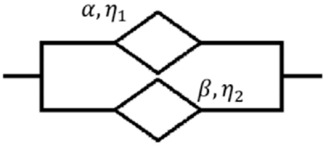
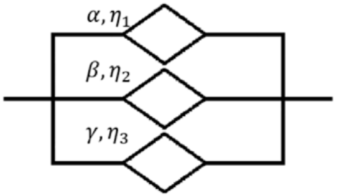
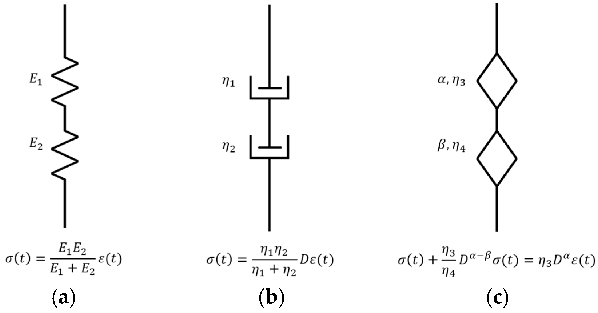
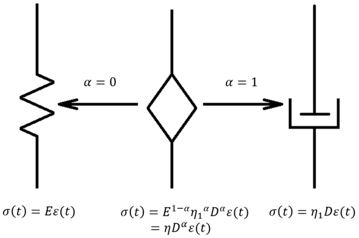
Koeller referred to the fractional rheological element as a “spring-pot” and represented it by using a diamond-shaped symbol [16], as shown in Figure 1. This element is typically characterized by two parameters: η , which is often interpreted as the “firmness” of a material [26,27], and the fractional order α , with α [ 0 , 1 ] . When α = 0 , the element reduces to an elastic spring; when α = 1 , it reduces to a dashpot.
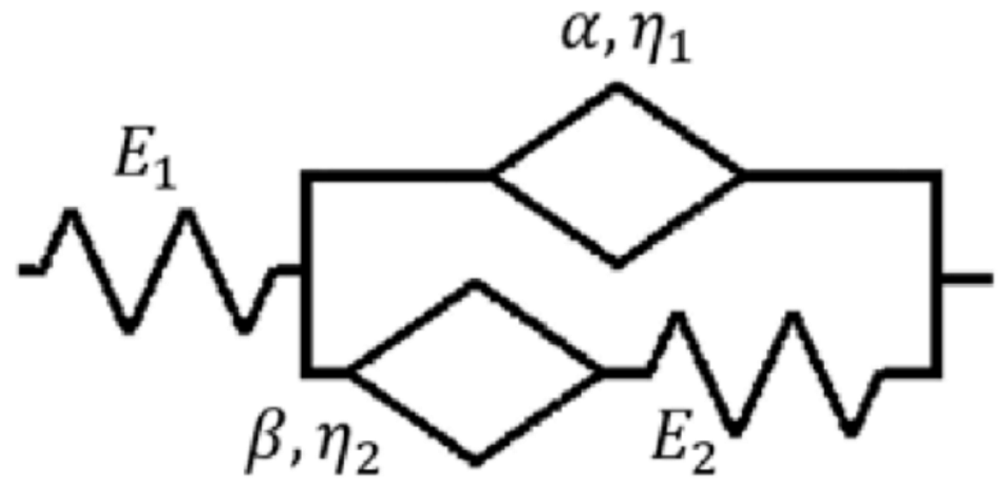
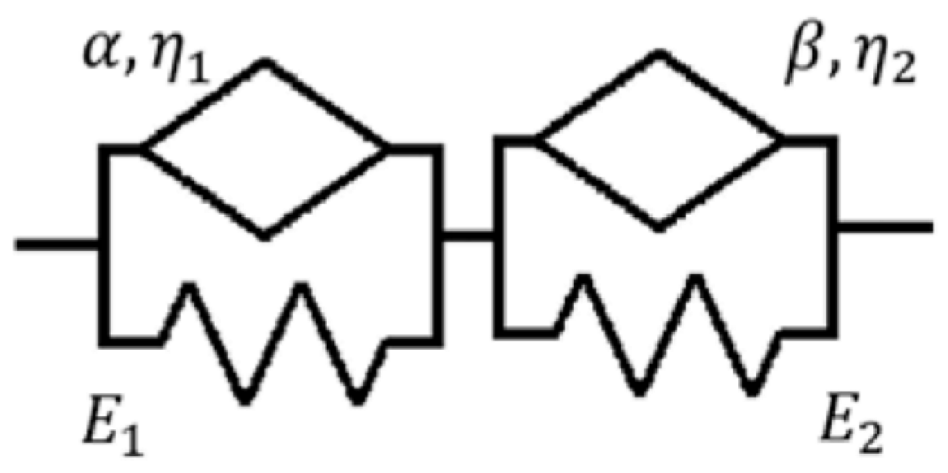
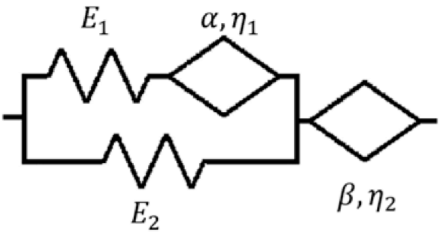
A notable distinction arises when considering combinations of individual rheological elements. For classical elements, combinations of springs alone or dashpots alone do not introduce additional time-dependent characteristics: springs remain purely elastic, while dashpots remain purely viscous, regardless of their series or parallel configurations. In contrast, fractional rheological elements inherently exhibit intermediate behavior between elasticity and viscosity. As illustrated in Figure 2, their combinations can generate richer time-dependent responses and introduce additional flexibility in representing viscoelastic behavior.

3. Construction of Fractional Viscoelastic Models for Polymer-Based Energetic Materials

This section describes the construction and calibration procedure for the candidate fractional viscoelastic models. First, the candidate model space and screening criteria are defined. Next, the Laplace-domain derivations of creep compliance and relaxation modulus are illustrated through a representative model. Finally, the parameter identification strategy based on numerical inverse Laplace transformation with a bio-inspired optimization algorithm is presented.

3.1. Fractional Viscoelastic Models for Polymer-Based Energetic Materials

In principle, fractional viscoelastic models can be assembled through arbitrary combinations of springs and spring-pots [15,19]. However, excessive complexity substantially increases computational cost and hinders parameter identifiability. In particular, Liu et al. referred to models containing three fractional rheological elements together with additional components as high-order fractional viscoelastic constitutive models [28]. The relaxation modulus expressions of their higher-order fractional models contain series terms and Mittag-Leffler functions with intricate parameters.
To balance descriptive capability, parameter efficiency, and engineering applicability, the candidate model space is restricted by two criteria: the number of rheological elements n 4 , and the number of model parameters m 6 .
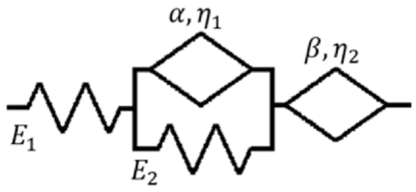
These criteria were used to retain compact fractional viscoelastic models while excluding higher-order models that may introduce excessive parameter complexity, strong parameter coupling, reduced identifiability, and unstable long-term extrapolation. Degenerate configurations and models reducible to simpler equivalent forms were also excluded, yielding 14 representative fractional viscoelastic models for subsequent investigation. Their mechanical analogs, constitutive equations, and Laplace-domain expressions are summarized in Appendix A.
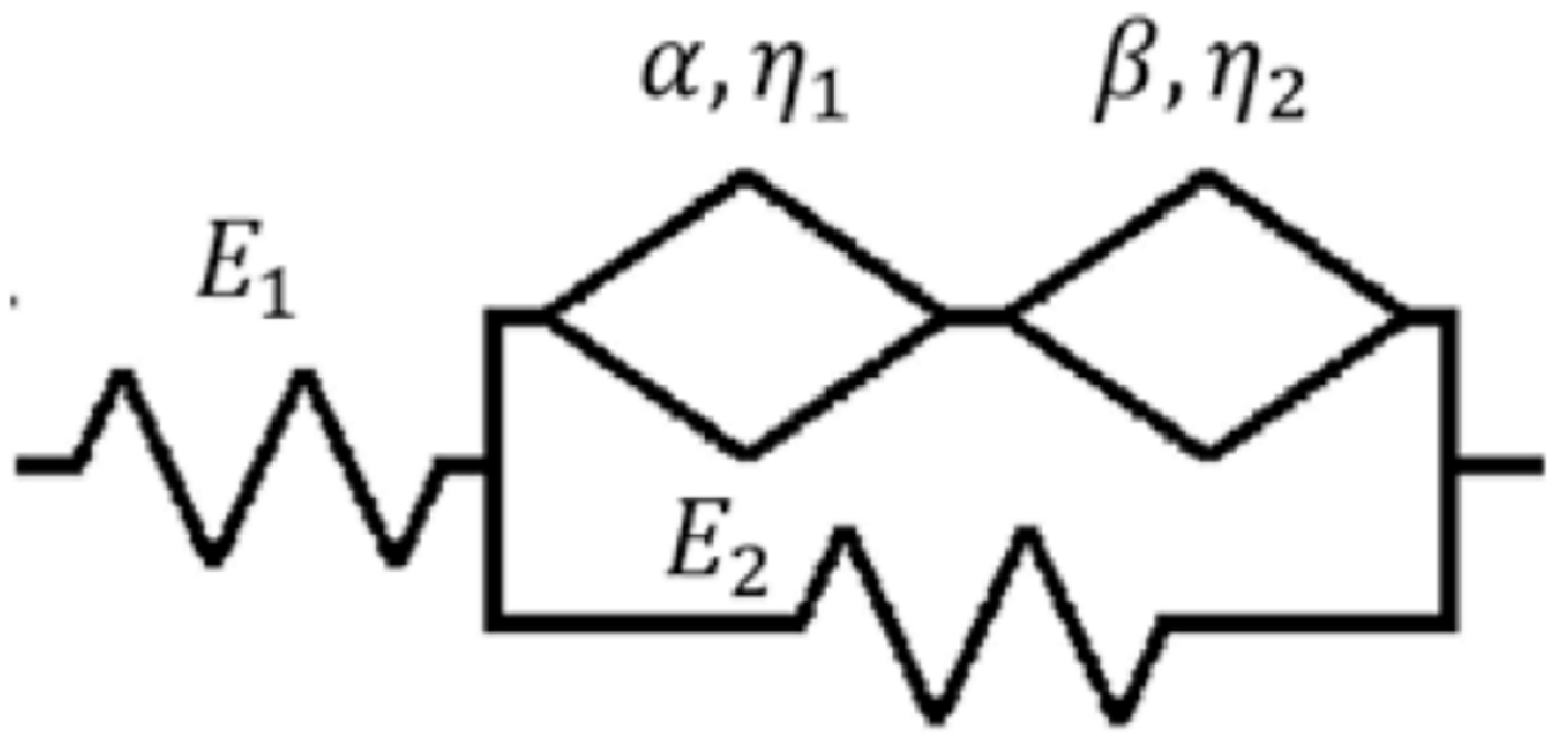
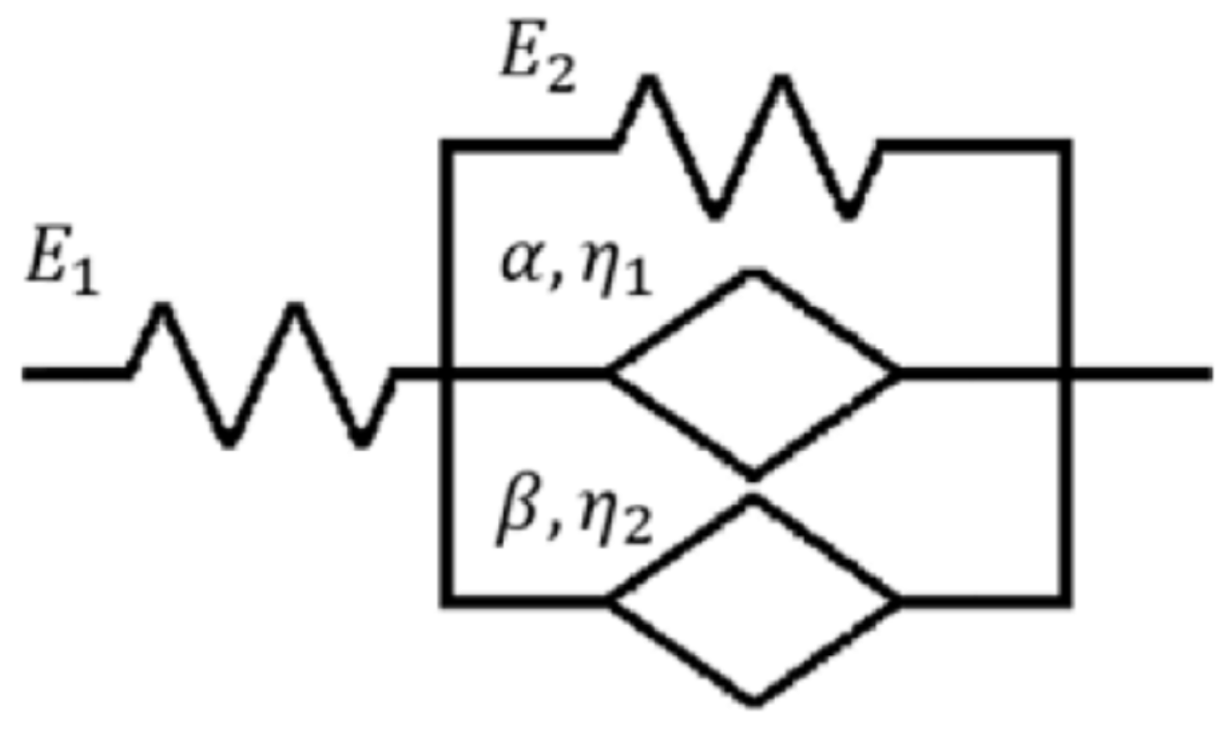
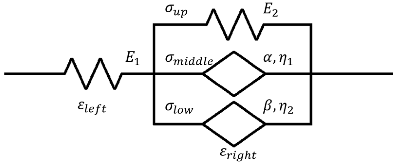
Because closed-form time-domain solutions are generally unavailable for these models, the Laplace-domain formulation coupled with numerical inversion is adopted as the principal solution strategy. To exemplify the derivation procedure, a six-parameter fractional model (Model 13) considered in this study is introduced below. As shown in Figure 3, this model comprises two classical springs ( E 1   , E 2 ) and two spring-pots ( η 1 ,   α ;   η 2 , β ) arranged in a specific series-parallel configuration.
The left branch contains only the spring E 1 , while the right branch consists of three parallel sub-branches: a spring E 2 and two spring-pots, ( η 1 ,   α ) and ( η 2 , β ). Let ε left ( t ) and ε right ( t ) denote the strains in the left and right parts of the model, respectively, and let σ up ( t ) , σ middle ( t ) , and σ low ( t ) represent the stresses in the upper, middle, and lower branches on the right, respectively. The kinematic and equilibrium relations hold as follows.
The total stress is equal to the sum of the stresses in the three branches on the right part:
σ ( t ) = σ u p ( t ) + σ m i d d l e ( t ) + σ l o w ( t ) .
The total strain is given by
ε ( t ) = ε l e f t ( t ) + ε r i g h t ( t ) .
For the two springs, Hooke’s law gives
σ ( t ) = E 1 ε l e f t ( t ) ,
σ u p ( t ) = E 2 ε r i g h t ( t ) .
For the two fractional rheological elements, the constitutive relations are
σ m i d d l e ( t ) = η 1 D α ε r i g h t ( t ) ,
σ l o w ( t ) = η 2 D β ε r i g h t ( t ) .
Applying the Laplace transform to Equations (6)–(8) yields
E r i g h t ( s ) = Σ ( s ) · 1 E 2 + η 1 s α + η 2 s β ,
E l e f t ( s ) = Σ ( s ) · 1 E 1 .
Combining Equations (9) and (10), the Laplace-domain constitutive relation of Model 13 is obtained as
E ( s ) = Σ ( s ) · E 1 + E 2 + η 1 s α + η 2 s β E 1 E 2 + E 1 η 1 s α + E 1 η 2 s β ,
where E r i g h t ( s ) , E l e f t ( s ) , and Σ ( s ) denote the Laplace transforms of ε r i g h t ( t ) , ε l e f t ( t ) , and σ ( t ) , respectively. Taking the inverse Laplace transform of Equation (11) gives
σ ( t ) + η 1 E 1 + E 2 D α σ ( t ) + η 2 E 1 + E 2 D β σ ( t ) = E 1 E 2 E 1 + E 2 ε ( t ) + E 1 η 1 E 1 + E 2 D α ε ( t ) + E 1 η 2 E 1 + E 2 D β ε ( t ) .
Equation (12) is the constitutive differential equation of Model 13. The same Laplace-domain procedure is applied to all 14 candidate models listed in Appendix A.

3.2. Expressions of Creep Compliance and Relaxation Modulus

Based on the Caputo fractional derivative, the Laplace-domain expressions for the creep compliance and relaxation modulus of Model 13 are derived using the Laplace transform.
Under zero initial conditions, all model variables and their derivatives vanish at t   = 0 . For a step stress σ 0 H ( t ) applied at t   =   0 , the stress input can be written as
σ ( t ) = σ 0 H ( t ) ,
where H ( t ) denotes the Heaviside step function, and the Laplace transform of the stress input is
Σ ( s ) = σ 0 · 1 s .
Substituting Equations (13) and (14) into Equation (11) gives
E ( s ) = σ 0 · 1 s · E 1 + E 2 + η 1 s α + η 2 s β E 1 E 2 + E 1 η 1 s α + E 1 η 2 s β ,
from Equation (15), the Laplace-domain expression for the creep compliance J ( s ) is obtained as
J ( s ) = Ε ( s ) σ 0 = E 1 + E 2 + η 1 · s α + η 2 · s β E 1 E 2 · s + E 1 η 1 · s α + 1 + E 1 η 2 · s β + 1 .
Similarly, under a step strain applied at t = 0 , the strain input and its Laplace transform can be written as
ε ( t ) = ε 0 H ( t ) ,
Ε ( s ) = ε 0 · 1 s .
Substituting Equations (17) and (18) into Equation (11) yields the Laplace-domain expression for the relaxation modulus G ( s ) :
G ( s ) = Σ ( s ) ε 0 = E 1 E 2 + E 1 η 1 · s α + E 1 η 2 · s β ( E 1 + E 2 ) · s + η 1 · s α + 1 + η 2 · s β + 1 .
Following the procedure outlined above, the Laplace-domain expressions for the creep compliance and relaxation modulus of all 14 models listed in Appendix A were derived using the same approach.

3.3. Talbot–Gray Wolf Parameter Identification Procedure

Parameter identification for fractional viscoelastic models can be formulated as the minimization of the discrepancy between model responses and experimental data. Accordingly, the optimization problem considered here is defined as a bounded minimization problem for an error function. Since the number of data points is typically much larger than the number of model parameters, the error function is defined as the sum of the squared relative errors between model responses and experimental data [22]:
E r r = i = 1 n [ f n u m ( x , t i ) y i y i ] 2 ,
where n denotes the number of discrete data points, x = [ x 1 , x 2 , , x m ] is the model parameter vector, t i is the time at the i -th data point, f num ( x , t i ) is the model response at time t i for the parameter vector x , and y i represents the actual value at time t i . The creep and relaxation datasets of polymer-based energetic materials are denoted uniformly by y i . All model parameters are taken to be non-negative, and the fractional-order parameters are constrained to α [ 0 , 1 ] , where the closed interval is adopted to include the degenerate cases of fractional rheological elements.
The expressions for creep compliance and relaxation modulus in many fractional viscoelastic models typically involve the Mittag-Leffler function, which makes gradient-based parameter identification difficult. Consequently, parameter identification for such models has attracted considerable attention. Various approaches, including Bayesian algorithms, interior-point methods, and Powell’s algorithm [22,29,30,31,32,33], have been employed in studies involving fractional calculus or Mittag-Leffler-type functions. However, closed-form time-domain expressions for most of the 14 models considered here are difficult to obtain, which further complicates parameter identification.
To address this issue, a parameter identification procedure combining the Talbot inverse Laplace method with the Gray Wolf Optimizer was adopted [34,35,36]. The numerical inverse Laplace method provides sufficient accuracy for engineering applications while reducing computational cost, and the Gray Wolf Optimizer is well-suited to gradient-free optimization problems. The overall optimization procedure is summarized in Algorithm 1.
Algorithm 1. Talbot–Gray Wolf parameter identification procedure
1:Generate an initial population of gray wolves X i   ( i = 1 ,   2 , ,   N )
2:Initialize the control parameters and termination condition
3:while (termination condition is not met) do
4:         For  each   wolf   X i  do
5:                   Compute the model response using the Talbot inverse Laplace method
6:                   Evaluate the objective function E r r ( X i ) using the experimental data
7:          end for
8:          Rank the wolves according to  E r r ( X i )
9:          Update the leading wolves   X α ,   X β   and   X δ
10:          Update the positions of all wolves using the Gray Wolf Optimizer
11:end while
12: return   X α
The combined Talbot–Gray Wolf parameter identification procedure provides an effective strategy for parameter identification in the fractional viscoelastic models considered here. This framework was employed in all subsequent fitting and extrapolation analyses of fractional viscoelastic models. As shown in Table 1, to ensure reproducibility of the stochastic optimization, the random number generator was initialized with a fixed seed of 2025. The number of truncation terms in the Talbot inversion method was set to 64, and the Gray Wolf Optimizer was configured with a population size of 40 and a maximum of 500 iterations. The lower bounds of all parameters were set to 0, and the upper bounds of the fractional orders were fixed at 1, whereas those of the remaining parameters differed across datasets; the specific values are provided in the corresponding sections. Given the variations in material properties and loading conditions, no additional termination criteria were imposed in any of the subsequent parameter identification and calibration processes, so that the optimization was terminated solely upon reaching the maximum number of iterations.
The benchmark models, including the power-law model and the Prony series models, were identified using least-squares fitting with the same error definition as that used for the fractional models. For the Prony series models, the relaxation or retardation times were prescribed as uniformly spaced on a logarithmic time scale across the range, and the remaining coefficients were fitted accordingly. For the fitting comparison in Section 4, the coefficient of determination R 2 was used to quantify descriptive accuracy, while the Akaike information criterion (AIC) was introduced to account for differences in the number of fitted parameters. The AIC was calculated as A I C = n l n ( R S S / n ) + 2 k , where n is the number of data points, RSS is the residual sum of squares, and k is the number of fitted parameters. A lower AIC indicates a better balance between fitting accuracy and model complexity. AIC values were compared only among models fitted to the same dataset. For the extrapolation assessment in Section 5, rRMSE was used to quantify the deviation between the extrapolated and experimental responses, with the calibration portion excluded from the calculation.
To further examine parameter identification stability and possible parameter coupling, 30 independent optimization runs with different random streams were performed for a representative fractional model and dataset. The resulting parameter distributions, correlation matrix, fitted curves, and extrapolated curves are provided in Appendix D.

4. Characterization of Fitting Performance of Fractional Viscoelastic Models

This section evaluates the descriptive performance of fractional viscoelastic models in comparison with classical models by using literature data on the creep and relaxation of PBX and solid propellants. Among the 14 candidate models, the fractional Zener model (Model 6 in Appendix A, denoted as “FZM” in the figures) and Model 13 consistently exhibited favorable descriptive performance across the datasets and are, therefore, highlighted here. For comparison, the power-law model and the Prony series forms of the generalized Maxwell or generalized Kelvin models are also included as benchmarks. The identified model parameters are provided in Appendix B. In the following comparisons, R 2 , AIC, and residual plots are used together to evaluate fitting accuracy, parameter complexity, and error distribution.

4.1. Characterization of Relaxation Modulus

The Prony series representation is a standard tool in linear viscoelasticity. Its performance depends on the prescribed relaxation or retardation times, the number of terms, and the fitting or regularization strategy. Therefore, the present comparison should be interpreted under the adopted logarithmically spaced time-constant setting. For relaxation comparison, the empirical power-law model and the generalized Maxwell model in Prony series form are employed as benchmark models.
The Prony series expression for relaxation is given by
G ( t ) = E + i = 1 n E i exp ( t τ i ) ,
where E is the equilibrium modulus, and E i represents the modulus of the i -th Maxwell branch; τ i is the relaxation time of the i -th branch, and n is the number of Maxwell branches connected in parallel.
In addition, the empirical model for relaxation is given by
G ( t ) = A + B · t α ,
where A , B , and α are parameters to be determined.

4.1.1. Relaxation Modulus of Solid Propellant (PVC/AP)

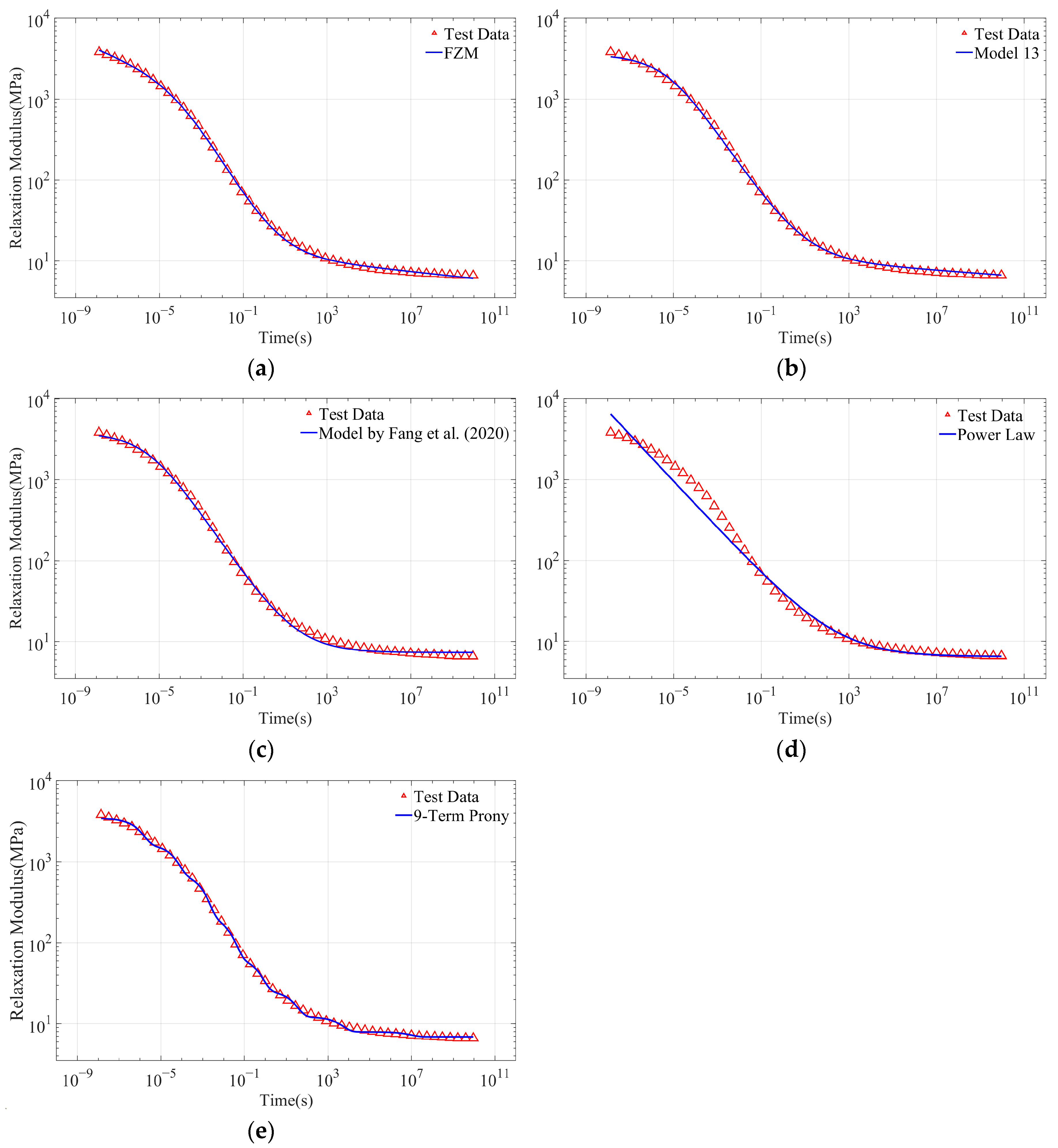
The relaxation master curve of a PVC/AP solid propellant was used to assess the models [37]. Fang et al. previously analyzed the same dataset using a five-element three-branch fractional Maxwell model and compared its performance with that of a 9-term Prony series [22]. The fractional Zener model, Model 13, the model of Fang et al., the power-law model, and the 9-term Prony series were evaluated comparatively. The upper bounds for all non-fractional-order parameters of fractional viscoelastic models were set to 10 4 . The corresponding fitting results are presented in Figure 4a–e and Table 2.
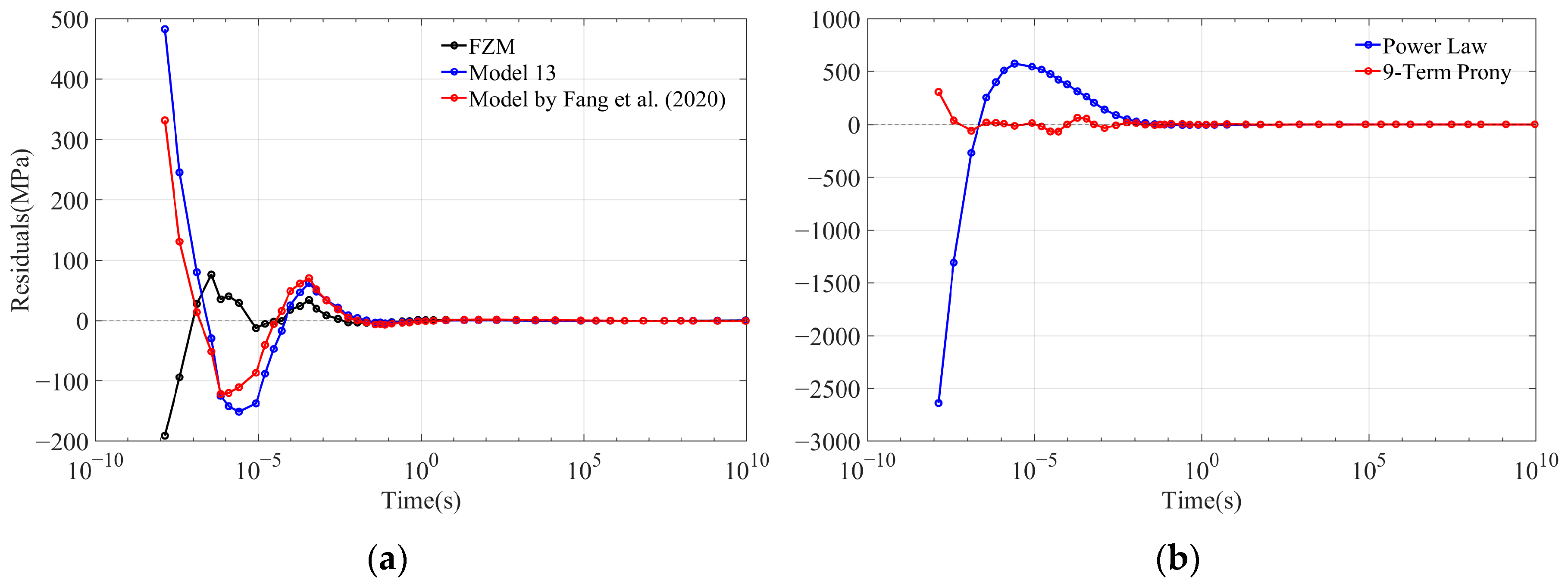
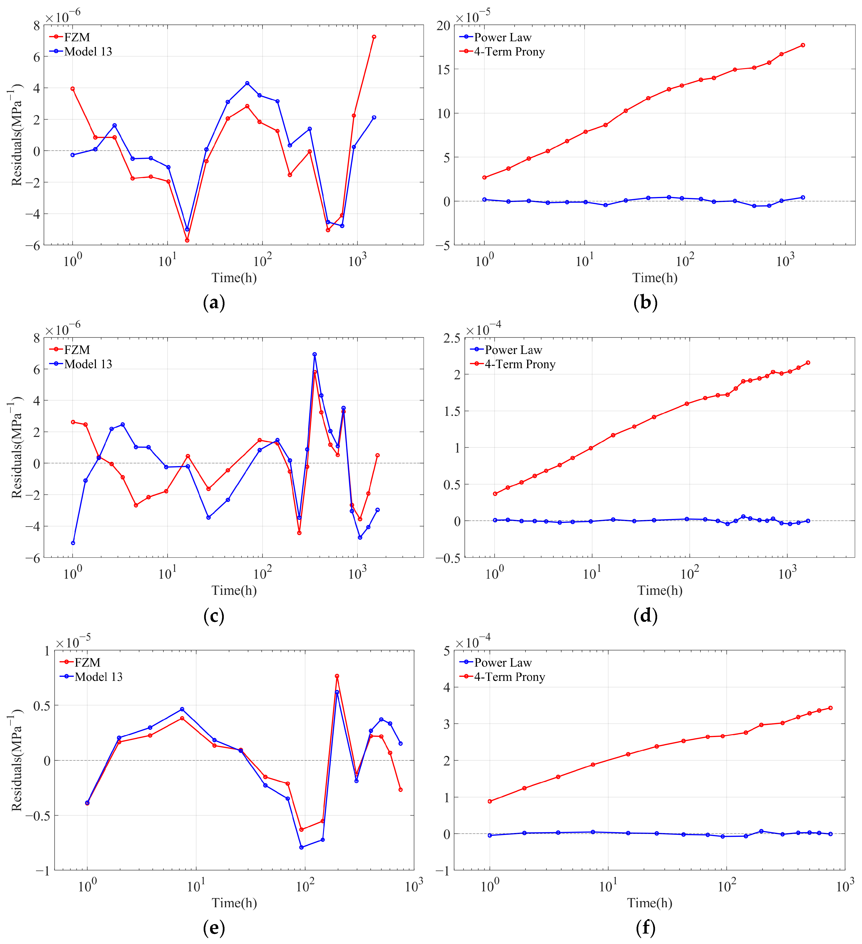
As summarized in Table 2, the fractional Zener model, Model 13, Fang et al.’s fractional model [22], and the 9-term Prony series all achieved high fitting accuracy ( R 2 > 0.99 ). The power-law model showed a much lower R 2 ( R 2 = 0.7772 ), indicating that it was less suitable for this relaxation dataset. When both fitting accuracy and parameter complexity are considered, the fractional Zener model ( m = 6 ) gave the lowest AIC among all compared models, suggesting the most favorable balance between accuracy and parameter economy for this dataset. Although the 9-term Prony series also achieved a high R 2 , it required a much larger number of parameters. Therefore, its complexity-penalized advantage was less pronounced than that of the fractional Zener model. Model 13 and Fang et al.’s fractional model [22] also provided accurate descriptions, but their AIC values were higher than that of the fractional Zener model in this case, which is consistent with the residual plots shown in Figure 5.
Given that the three-branch fractional Maxwell model falls outside the selection criteria of this study ( n 4 ,   m 6 ) and features a relatively complex expression for creep compliance, it was excluded from subsequent analyses.

4.1.2. Relaxation Modulus of PBX

Xiao et al. reported the short-term relaxation master curve data ( 10 4 10 4   s ) for PBX at 20   ° C [38]. For comparison, the fitting results of the two fractional viscoelastic models, together with those of the power-law model and the Prony series, were presented for the PBX relaxation data, and the upper bounds for all non-fractional-order parameters of the fractional viscoelastic models were set to 3000.
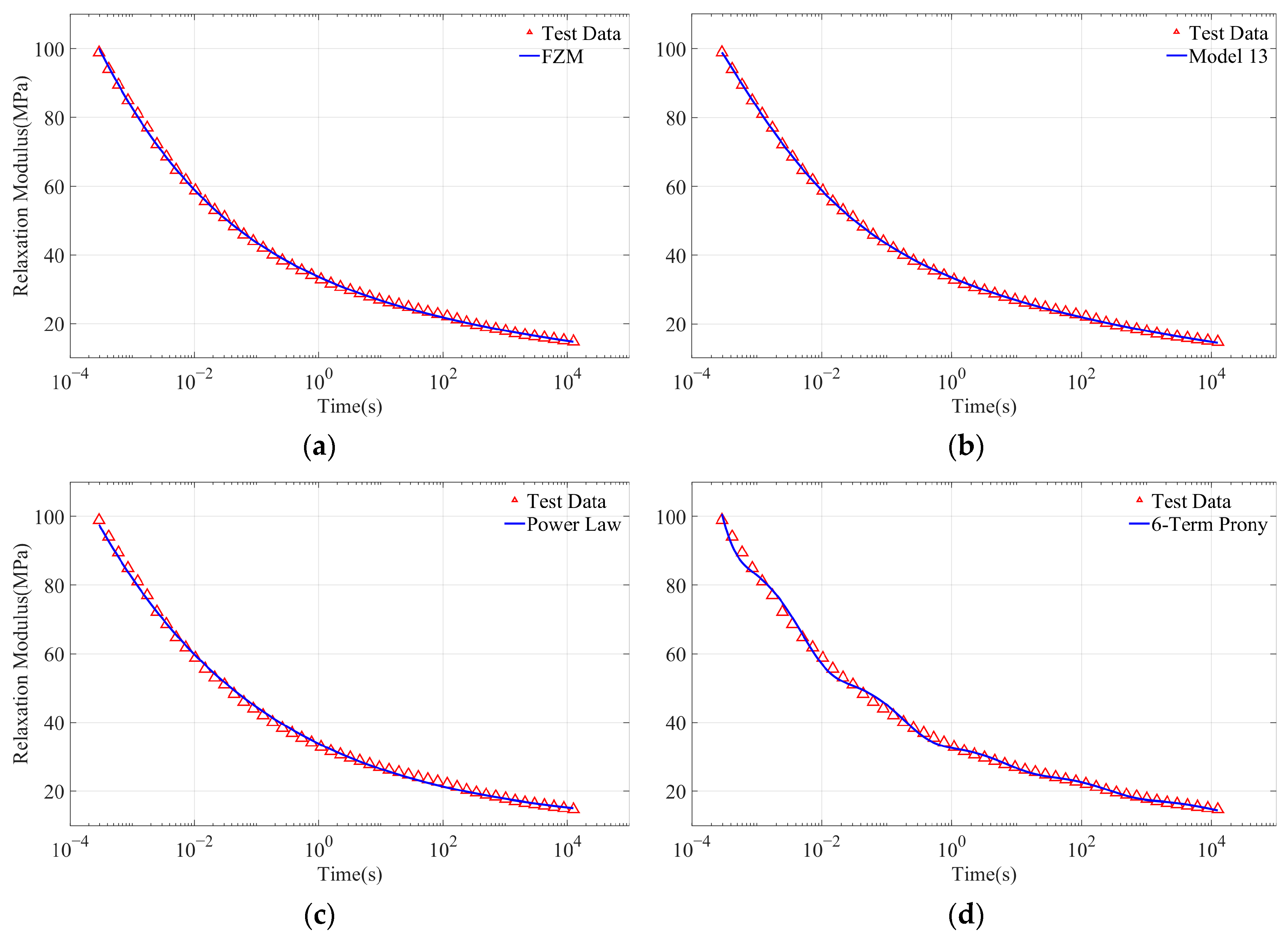
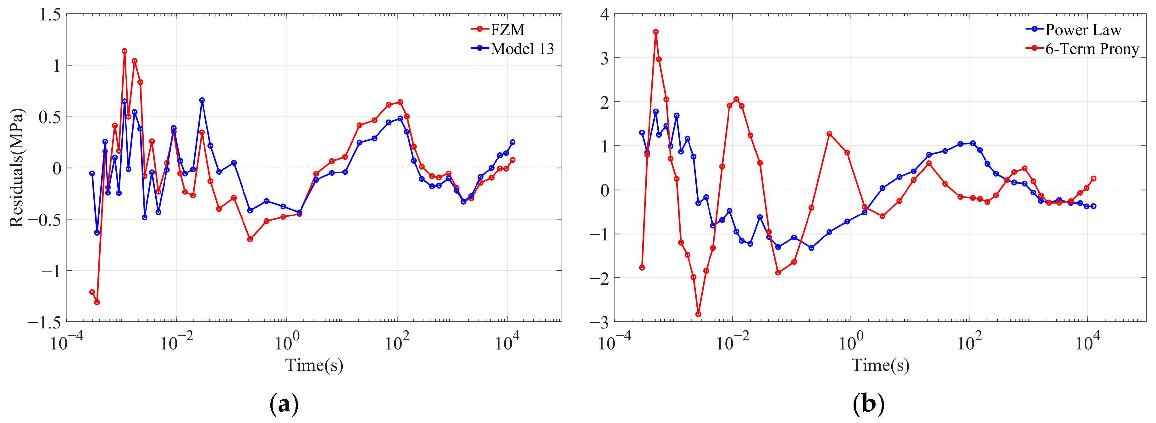
Figure 6 illustrates the fitted curves together with the experimental data. The two fractional viscoelastic models, as well as the power-law model and the 6-term Prony series, all accurately described the short-term relaxation behavior of PBX, with R 2 0.9977 . However, the residual plots in Figure 7 and the AIC values in Table 3 further distinguish their complexity-penalized performance. Model 13 achieved the lowest AIC, followed by the fractional Zener model, indicating that the two fractional models provided a better balance between fitting accuracy and parameter complexity than the Prony series models under the present fitting protocol. Although the 6-term Prony series also achieved high R 2 , its larger parameter number resulted in a less favorable AIC. These results support the use of compact fractional models for the short-term relaxation characterization of PBX.

4.2. Characterization of Creep Compliance

Consistent with the relaxation data, the creep data plotted on a logarithmic time scale were also obtained from the creep behavior of PBX and solid propellants. For comparison, the empirical power-law model for creep and the creep form of the generalized Kelvin model were employed. The expression of the Prony series for creep is given by
J ( t ) = 1 J 0 + i = 1 n 1 J i ( 1 exp ( t λ i ) ) ,
where 1 J 0 is the instantaneous compliance, and 1 J i represents the compliance of the i -th Kelvin branch, λ i is the retardation time of the i -th branch, and n is the number of Kelvin branches connected in series. Meanwhile, the empirical model for creep is given by
J ( t ) = A + B · t β ,
where A , B , and β are parameters to be determined.

4.2.1. Creep Compliance of PBX

Thompson et al. [39] systematically investigated the creep behavior of PBX 9502 under various temperatures and tensile/compressive loads. Here, creep data under axial loads of 3   MPa   ( 40   ° C ) , 4   MPa   ( 40   ° C ) , and 5   MPa   ( 50   ° C ) were employed for analysis. The data began at approximately 1 h; due to the absence of data in the glassy region ( t   <   10 0   s ), 3-term and 4-term Prony-series models were employed for fitting. The fitting results and residual plots for each model are shown in Figure 8 and Figure 9, respectively. The upper bounds for all non-fractional-order parameters of fractional viscoelastic models were set to 10 6 . For compressive creep data, the creep compliance is reported as a positive magnitude, calculated from the absolute values of strain and compressive stress; the same convention was used consistently in fitting, AIC calculation, and error evaluation.
All compared models achieved satisfactory fitting performance for the compressive creep data of PBX, with R 2 values of at least 0.9971. As summarized in Table 4, the two fractional models accurately captured the creep behavior under all three loading conditions. However, when AIC is considered, the advantage of the fractional models becomes less uniform than that observed in the relaxation cases. The power-law model gave the lowest AIC at −3 MPa and −4 MPa, while the 4-term Prony series gave the lowest AIC at −5 MPa. This indicates that the PBX compressive creep curves considered here can also be efficiently represented by empirical or low-order Prony series models, especially because the data cover mainly the longer-time regime and exhibit nearly smooth trends on the logarithmic time scale. Nevertheless, the fractional Zener model and Model 13 maintained consistently high R 2 values with a limited number of parameters, showing stable descriptive capability across all three compressive creep conditions.

4.2.2. Creep Compliance of Solid Propellant (NEPE)

The creep data for solid propellants were obtained from Zhang et al. [40], who investigated the creep behavior of NEPE under different loads and loading durations. They reported that the yield stress of NEPE was approximately 0.2 0.25   MPa . Accordingly, creep data under a load of 0.15   MPa with a loading duration of about 10 6   s were selected for analysis. Due to the absence of data in the glassy region ( t   <   10 0   s ), 3-term and 4-term Prony series were employed to fit the creep data. The upper bounds for all non-fractional-order parameters of fractional viscoelastic models were set to 10 6 .
As illustrated in Figure 10a,b,d, the two fractional models and the 4-term Prony series reasonably described the creep compliance of NEPE. Table 5 shows that these models achieved high fitting accuracy, with R 2 0.9964 , the residual plots in Figure 11 also demonstrate the satisfactory fit achieved by these models. Among them, Model 13 achieved the highest R 2 and the lowest AIC, indicating the best balance between fitting accuracy and parameter complexity for this dataset. The fractional Zener model and the 4-term Prony series also showed satisfactory performance, whereas the power-law model showed both a lower R 2 value and a less favorable AIC. These results suggest that Model 13 is particularly suitable for the low-rate creep response of NEPE considered here.

4.3. Summary and Discussion of Fitting Performance

Based on the R 2 in Appendix B, as well as the residual plots and AIC values presented in Figure 5, Figure 7 and Figure 9, and 11, Table 2, Table 3, Table 4 and Table 5, several low-parameter fractional models were able to describe both creep and relaxation responses of polymer-based energetic materials with high accuracy. In particular, the fractional Zener model and Model 13 were able to describe both creep compliance and relaxation modulus within compact rheological forms with a limited number of parameters while maintaining stable performance across different time scales. Therefore, three fractional viscoelastic models, namely the fractional Zener model, the fractional Poynting–Thomson model (Model 5 in Appendix A), and Model 13, together with the same benchmark models, were used for the assessment in the next section.
The inclusion of AIC provides a more balanced comparison among models with different parameter complexities. For the relaxation datasets, the fractional Zener model and Model 13 generally showed favorable complexity-penalized performance, indicating that compact fractional models are suitable for representing broad viscoelastic relaxation behavior. For the creep datasets, the AIC results suggest that the advantage of fractional models depends on the material response and data characteristics. In the PBX compressive creep cases, the power-law model or the 4-term Prony series achieved the lowest AIC under some loading conditions, whereas the fractional models maintained consistently high R 2 values with limited parameter numbers. Therefore, the advantage of fractional viscoelastic models should not be interpreted as universal superiority over Prony series or power-law models. Their main value lies in providing compact rheological representations for both creep and relaxation responses, with good overall accuracy and reduced parameter complexity.
The fitted responses were also checked for basic physical admissibility over the time windows of the literature data. With non-negative moduli and spring-pot coefficients and fractional orders constrained within [0, 1], the fitted relaxation moduli remained positive and non-increasing, while the fitted creep compliances remained positive and non-decreasing in magnitude. These numerical checks support the physical admissibility of the selected parameter sets within the considered data range, although they do not constitute full thermodynamic proof for arbitrary loading histories.

5. Assessment of Extrapolation Behavior from Early-Stage Data

In this section, early-stage data were used for calibration to assess the extrapolation behavior of selected models. Specifically, the first 10% of the time span of each dataset was used for parameter identification, and the subsequent long-time response was used to evaluate extrapolation performance. The complete curves are shown in the figures for visual comparison, and the corresponding parameters and rRMSE values are provided in Appendix B.

5.1. Extrapolation of Relaxation Modulus

5.1.1. Extrapolation of Solid Propellant Relaxation Data (PVC/AP)

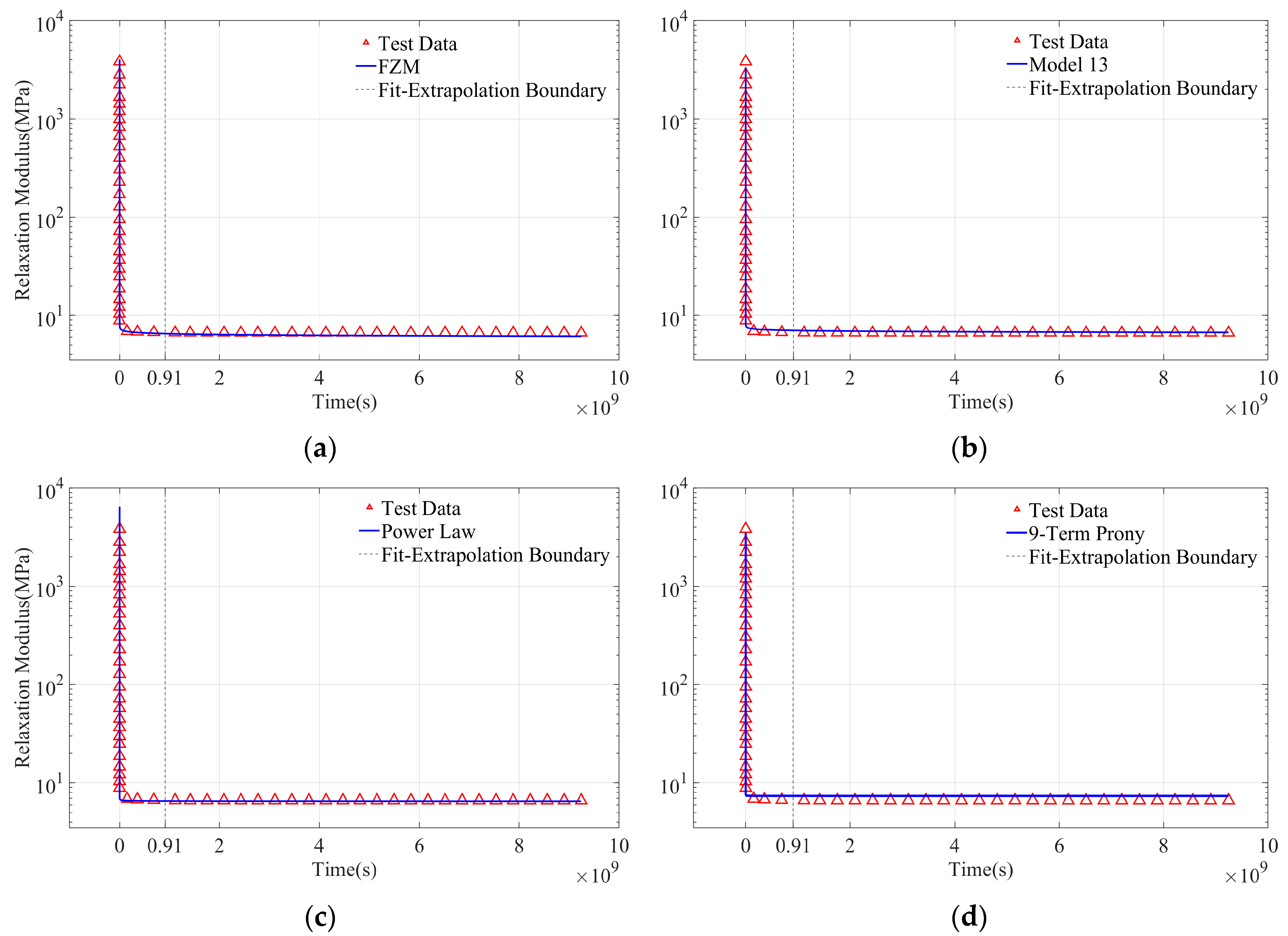
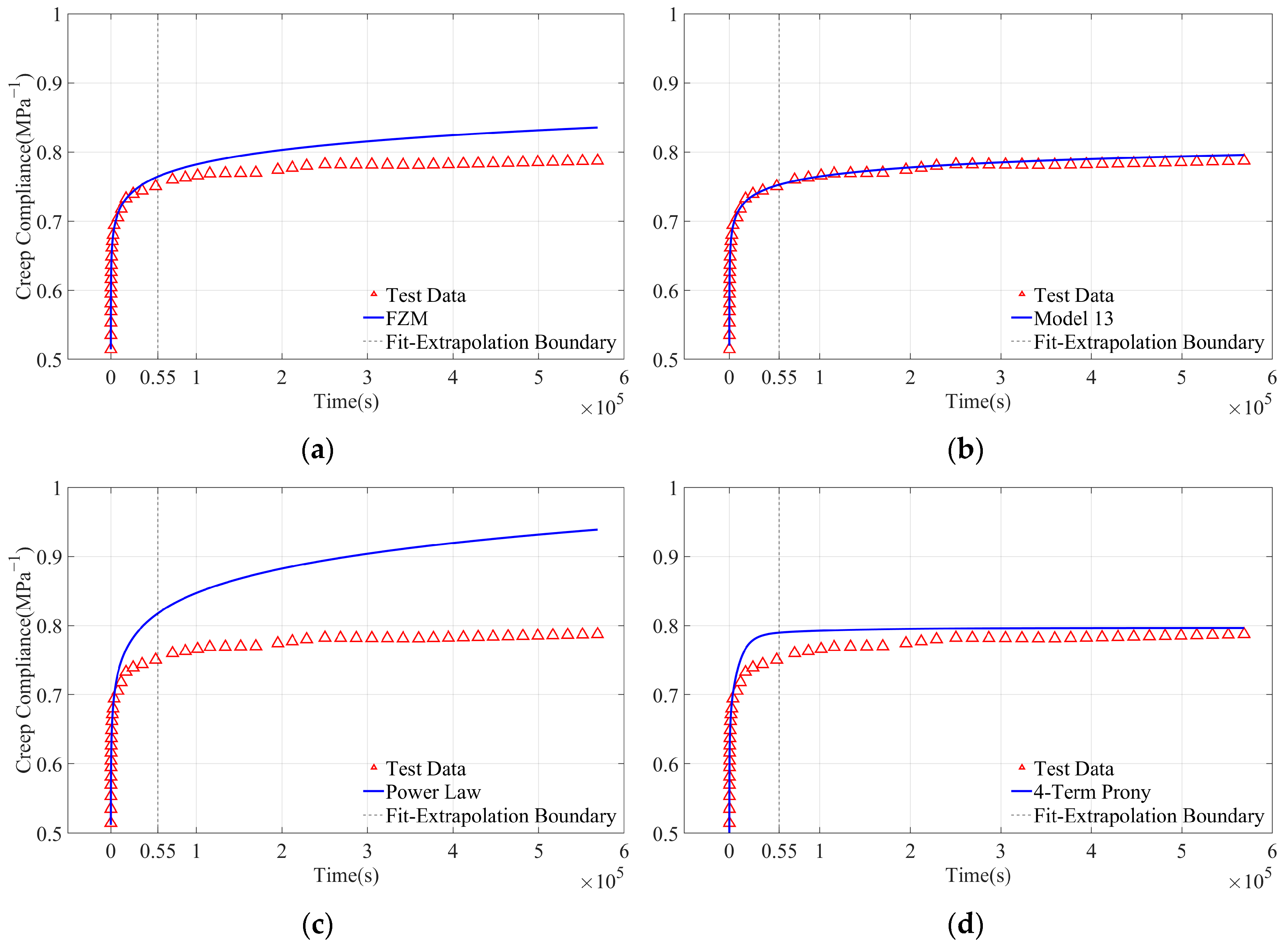
In the extrapolation of the PVC/AP relaxation data, the fractional Zener model achieved R 2 = 0.9922 and r R M S E = 5.78 % , while Model 13 achieved R 2 = 0.9915 and r R M S E = 3.45 % , as shown in Figure 12 and Table 6. By contrast, although the power-law model yielded the lowest extrapolation error ( r R M S E = 1.63 % ), its relatively low coefficient of determination ( R 2 = 0.7776 ) indicated that it did not adequately capture the overall shape of the relaxation curve. The 9-term Prony series achieved both a high R 2 value ( R 2 = 0.9952 ) and a low r R M S E ( 1.88 % ). Overall, the two fractional viscoelastic models combined consistently high R 2 values with acceptable extrapolation errors, indicating stable extrapolation behavior within the considered dataset.
At sufficiently long times, all exponential terms in the Prony series decay to zero, causing the extrapolated curve to approach a horizontal asymptote. For polymer-based energetic materials in the rubbery state, the stress decay rate is inherently very low. The extrapolation performance of the Prony series model should be interpreted within the adopted fitting protocol, because it depends strongly on the prescribed relaxation times, the number of terms, and possible regularization strategies.

5.1.2. Extrapolation of PBX Relaxation Data

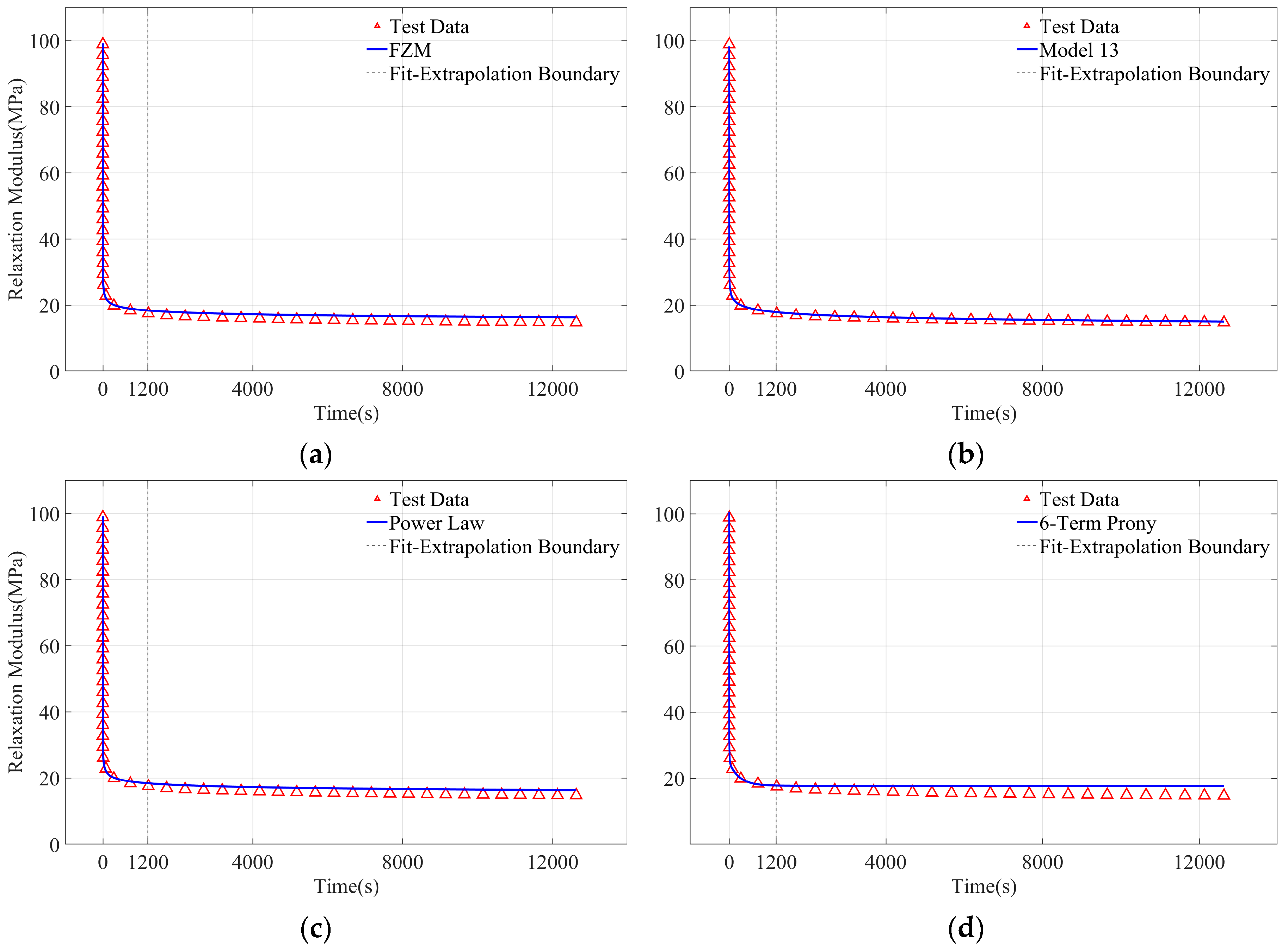
Similarly, when the first 10% of the time span was used for parameter identification, as Table 7 indicate, both fractional models and the power-law model achieved favorable extrapolation performance for the relaxation master curve of PBX ( r R M S E 8.45 % ). The 6-term Prony series still achieved a high R 2 value but showed a larger quantitative extrapolation error ( r R M S E = 13.21 % ), while the lower-term Prony series exhibited unsatisfactory results ( r R M S E 33.37 % ). In contrast, the extrapolated curves of the two fractional models were closer to the experimental data, and the power-law model showed similar extrapolative capability, while the Prony series exhibited unstable performance. As shown in Figure 13, the extrapolated curve of the Prony series displayed a near-zero stress rate in the rubbery region, which deviated from the observed relaxation trend in the rubbery region.

5.2. Extrapolation of Creep Compliance

5.2.1. Extrapolation of PBX Creep Data

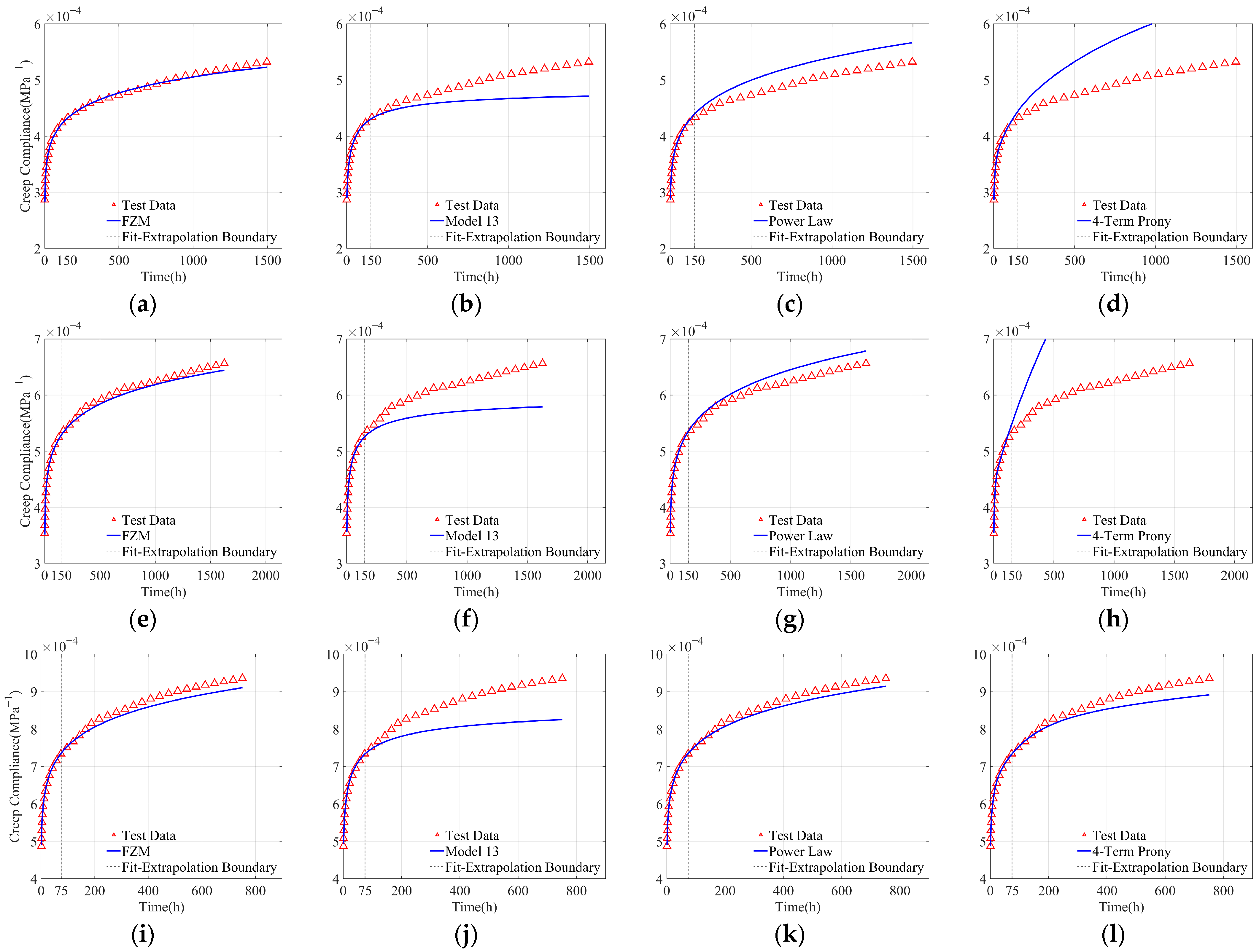
As shown in Figure 14 and Table 8, when extrapolating the compressive creep data of PBX under loads of 3   MPa , 4   MPa , and 5   MPa , the fractional Zener model achieved the best and most stable extrapolation performance, with consistently high coefficients of determination ( R 2 0.9943 ) and low extrapolation errors ( r R M S E 1.74 % ) under all three conditions. The power-law model also showed reasonably good extrapolative capability, with r R M S E values ranging from 1.84 % to 5.34 % , although its overall stability across the three conditions remained inferior to that of the fractional Zener model. By contrast, Model 13 yielded less satisfactory results, with relatively low R 2 values ( 0.8767 R 2 0.9348 ) and higher rRMSE values ( 6.73 % r R M S E 8.19 % ). Among the Prony series models, the 3-term Prony series exhibited consistently poor extrapolation performance, with negative R 2 values at 3   MPa and 4   MPa and large extrapolation errors ( r R M S E 13.08 % ), while the 4-term Prony series performed better but remained unstable, with r R M S E values ranging from 3.11 % to 34.44 % . In particular, the 4-term Prony series achieved acceptable results at 5   MPa ( R 2 = 0.9822 , r R M S E = 3.11 % ), its extrapolation performance deteriorated markedly at the lower load levels. Notably, although Model 13 did not achieve satisfactory extrapolation performance under these three conditions, its extrapolated curves consistently exhibited relatively low steady-state creep rates.

5.2.2. Extrapolation of Solid Propellant Creep Data (NEPE)

In the case of NEPE creep extrapolation, as shown in Figure 15 and Table 9, Model 13 achieved favorable extrapolation performance ( r R M S E = 0.56 % ), comparable to that of the 4-term Prony series ( r R M S E = 0.33 % ), and significantly better than the fractional Zener model ( r R M S E = 3.65 % ), while the power-law model exhibited the poorest extrapolation performance ( r R M S E = 13.45 % ). These results indicate that Model 13 is particularly suitable for materials characterized by low strain rates during the steady-state creep stage. Although the 4-term Prony series also achieved a low extrapolation error, its extrapolated curve exhibited a distinct linear trend in the steady-state creep regime, suggesting that, under the present fixed time-constant setting, the generalized Kelvin model may produce an overly linear extrapolation trend in the steady-state creep regime. By contrast, Model 13 provided both high extrapolative accuracy and a smoother description of the low-rate steady-state creep response.

5.3. Summary and Discussion of Extrapolation Behavior

According to Figure 12, Figure 13, Figure 14 and Figure 15, and the R 2 , rRMSE in Table 6, Table 7, Table 8 and Table 9 and Appendix B, the extrapolation results indicate that the fractional Zener model and Model 13 provide different advantages depending on the material response. For relaxation data, both models gave stable extrapolation within the considered datasets. For creep data, the fractional Zener model was more suitable for cases with relatively high steady-state creep rates, whereas Model 13 performed better for low-rate creep responses. The Prony series models also showed excellent performance in some cases, especially when sufficient terms were used. However, their extrapolation behavior depended on the prescribed time constants and the number of terms. The power-law model remains useful as an engineering approximation for datasets exhibiting approximately power-law trends, but it lacks a direct rheological analog for unified creep-relaxation interpretation.
Since only the first 10% of the time span was used for calibration, the extrapolation assessment corresponds to an approximately one-order-of-magnitude extension in the time window within the available experimental curves. This setting provides a practical test of early-stage data extrapolation, although it should not be interpreted as independent experimental validation.
It should also be noted that the present assessments were restricted to linear viscoelastic models. The relaxation datasets considered in this study were master curves constructed using the time–temperature superposition principle, which is commonly applied within the small-strain linear viscoelastic framework. However, because the published datasets do not always provide multi-level creep or relaxation curves, the linear viscoelastic assumption cannot be independently verified for all cases, especially under relatively high compressive loading conditions. Possible nonlinear viscoelastic effects at higher stress or strain levels may lead to load-dependent parameters and reduce the reliability of extrapolation outside the calibrated loading condition.
The fractional parameters identified in this study should be interpreted as phenomenological quasi-properties rather than direct microstructural descriptors. The fractional orders may reflect the combined effects of binder viscoelasticity, particle–binder interfacial interactions, particle-packing heterogeneity, and distributed relaxation mechanisms. Nevertheless, the present macroscopic creep and relaxation data do not allow a definitive correspondence between individual fractional parameters and specific microstructural features to be established. Establishing such a relationship would require additional microstructural characterization and multiscale mechanical analysis.
In addition, an in-house PBX creep dataset was further analyzed, and the results are provided in Appendix C. The supplementary results show similar trends in model performance and provide an additional consistency check for the applicability of the selected fractional models to PBX creep data. However, this supplementary analysis should not be interpreted as complete independent validation over all material systems, loading conditions, or experimental uncertainties.


6. Conclusions

This study compared low-parameter fractional viscoelastic models for describing and extrapolating creep and stress relaxation behaviors of polymer-based energetic materials. Fourteen candidate models composed of springs and spring-pot elements were considered under controlled parameter complexity, and their performance was evaluated using PBX and solid propellant datasets. The main conclusions are as follows:
(1)
Among the 14 candidate models, the fractional Zener model and Model 13 showed the most favorable overall performance for the datasets considered. These two models can describe both creep compliance and stress relaxation modulus within compact six-parameter rheological forms, with coefficients of determination generally exceeding 0.99. Compared with high-order Prony series models in the relaxation cases, they achieved comparable fitting accuracy with lower parameter complexity.
(2)
The combined Talbot–Gray Wolf parameter identification procedure provided a practical parameter identification route for fractional viscoelastic models without analytical time-domain solutions. With the numerical settings specified in this study, the procedure successfully identified parameters for the candidate models. Repeated optimization results in Appendix D further indicate that the identified parameters remained within bounded ranges for the representative case considered.
(3)
When the first 10% of the time span was used for calibration, the selected fractional models showed reasonable extrapolation behavior over an approximately one-order-of-magnitude longer time window within the available experimental curves. The rRMSE values of the fractional Zener model and Model 13 were below 8.5% in the reported extrapolation cases, and below 2% under their respective suitable conditions.
(4)
The comparison with Prony series and power-law models shows that compact fractional models provide useful alternatives for representing broad viscoelastic response behavior. Prony series models remain standard tools in linear viscoelasticity, but their extrapolation behavior depends on the prescribed relaxation or retardation times and the number of terms. The power-law model can still serve as an engineering approximation for approximately power-law responses, although it lacks a direct rheological analog for unified creep-relaxation interpretation.
(5)
In addition to published datasets, an in-house PBX creep dataset was analyzed as a supplementary check in Appendix C. The supplementary results showed similar trends in model performance and provided an additional consistency check for the applicability of the selected fractional models to PBX creep analysis.
The present work should be interpreted as a comparative model assessment based mainly on published datasets, rather than as complete independent experimental validation. Future work should therefore combine controlled multi-level experiments, normalized relaxation or creep curve comparisons, nonlinear viscoelastic modeling, and broader parameter identifiability analyses to further assess the model transferability and applicability.

Author Contributions

Conceptualization, H.Y. and W.T.; methodology, H.Y. and D.G.; software, D.G.; validation, D.G.; formal analysis, D.G. and H.Y.; investigation, D.G. and L.Z.; data curation, L.Z.; writing—original draft preparation, D.G.; writing—review and editing, H.Y.; visualization, D.G.; supervision, H.Y. and W.T. All authors have read and agreed to the published version of the manuscript.

Funding

This research was supported by the Science Challenge Project (No. TZ2025010).

Institutional Review Board Statement

Not applicable.

Data Availability Statement

The data used in this study are available from the cited references and the supplementary tables in the Appendix.

Conflicts of Interest

The authors declare no conflicts of interest.

Appendix A. Candidate Fractional Viscoelastic Models

This appendix summarizes the 14 candidate fractional viscoelastic models considered in this study. For each model, the mechanical analog, differential constitutive equation, creep compliance, and relaxation modulus are provided, as shown in Table A1. These models were constructed under the complexity constraint adopted in the main text, and degenerate configurations reducible to simpler equivalent forms were excluded.
Table A1. Summary of the 14 fractional viscoelastic models: mechanical analogs, differential constitutive relations, creep compliances, and relaxation moduli.
ModelDifferential Constitutive EquationCreep ComplianceRelaxation Modulus
Polymers 18 01430 i001 σ + η 1 η 2 D α β σ = η 1 D α ε J ( t ) = 1 η 1 t α Γ ( 1 + α ) + 1 η 2 t β Γ ( 1 + β ) G ( t ) = η 2 · t β · E α β , 1 β ( η 2 η 1 · t α β )
Model 1
Polymers 18 01430 i002 σ = η 1 D α ε + η 2 D β ε J ( t ) = 1 η 1 · t α · E α β , 1 + α ( η 2 η 1 · t α β ) G ( t ) = η 1 · t α Γ ( 1 α ) + η 2 · t β Γ ( 1 β )
Model 2
Polymers 18 01430 i003 σ + η 1 η 2 D α β σ + η 1 η 3 D α γ σ = η 1 D α ε J ( t ) = 1 η 1 t α Γ ( 1 + α ) + 1 η 2 t β Γ ( 1 + β ) + 1 η 3 t γ Γ ( 1 + γ ) G ( s ) = η 1 η 2 η 3 · s α + β + γ η 1 η 2 · s α + β + 1 + η 1 η 3 · s α + γ + 1 + η 2 η 3 · s β + γ + 1
Model 3
Polymers 18 01430 i004 σ = η 1 D α ε + η 2 D β ε + η 3 D γ ε J ( s ) = 1 η 1 · s α + 1 + η 2 · s β + 1 + η 3 · s γ + 1 G ( s ) = η 1 · t α Γ ( 1 α ) + η 2 · t β Γ ( 1 β ) + η 3 · t γ Γ ( 1 γ )
Model 4
Polymers 18 01430 i005 σ + η 2 η 1 D β α σ + η 3 η 1 D γ α σ = η 2 D β ε + η 3 D γ ε J ( t ) = 1 η 1 t α Γ ( 1 + α ) + 1 η 2 · t β · E β γ , 1 + β ( η 3 η 2 · t β γ ) G ( s ) = η 1 η 2 · s α + β + η 1 η 3 · s α + γ η 1 · s α + 1 + η 2 · s β + 1 + η 3 · s γ + 1
Model 5
Polymers 18 01430 i006 σ + η 2 η 1 D β α σ = η 2 D β ε + η 3 D γ ε + η 2 η 3 η 1 D β + γ α ε J ( s ) = η 1 · s α + η 2 · s β η 1 η 2 · s α + β + 1 + η 1 η 3 · s α + γ + 1 + η 2 η 3 · s β + γ + 1 G ( t ) = η 2 · t β · E α β , 1 β ( η 2 η 1 · t α β ) + η 3 · t γ Γ ( 1 γ )
Model 6
Polymers 18 01430 i007 σ + E 1 η 1 + E 2 η 1 E 1 η 1 + E 2 η 2 D α β σ + η 1 η 2 E 1 η 1 + E 2 η 2 D α σ = E 1 E 2 η 2 E 1 η 1 + E 2 η 2 ε + E 1 η 1 η 2 E 1 η 1 + E 2 η 2 D α ε + E 1 E 2 η 1 E 1 η 1 + E 2 η 2 D α β ε J ( s ) = ( E 1 η 1 + E 2 η 1 ) · s α + ( E 1 η 1 + E 2 η 2 ) · s β + η 1 η 2 · s α + β E 1 E 2 η 1 · s α + 1 + E 1 E 2 η 2 · s β + 1 + E 1 η 1 η 2 · s α + β + 1 G ( s ) = E 1 E 2 η 1 · s α + E 1 E 2 η 2 · s β + E 1 η 1 η 2 · s α + β ( E 1 η 1 + E 2 η 1 ) · s α + 1 + ( E 1 η 1 + E 2 η 2 ) · s β + 1 + η 1 η 2 · s α + β + 1
Model 7
Polymers 18 01430 i008 σ + η 1 E 2 D α σ + ( η 2 E 1 + η 2 E 2 ) D β σ + η 1 η 2 E 1 E 2 D α + β σ = η 2 D β ε + η 1 η 2 E 1 E 2 D α + β ε J ( s ) = E 1 E 2 + E 1 η 1 · s α + ( E 1 η 2 + E 2 η 2 ) · s β + η 1 η 2 · s α + β E 1 E 2 η 2 · s β + 1 + E 1 η 1 η 2 · s α + β + 1 G ( s ) = E 1 E 2 η 2 · s β + E 1 η 1 η 2 · s α + β E 1 E 2 · s + E 1 η 1 · s α + 1 + ( E 1 η 2 + E 2 η 2 ) · s β + 1 + η 1 η 2 · s α + β + 1
Model 8
Polymers 18 01430 i009 σ + η 2 E 2 D β σ = E 1 ε + η 1 D α ε + ( E 1 E 2 η 2 + η 2 ) D β ε + η 1 η 2 E 2 D α + β ε J ( s ) = E 2 + η 2 · s β E 1 E 2 · s + E 2 η 1 · s α + 1 + ( E 1 η 2 + E 2 η 2 ) · s β + 1 + η 1 η 2 · s α + β + 1 G ( t ) = E 1 + η 1 t α Γ ( 1 α ) + E 2 · E β , 1 ( E 2 η 2 t β )
Model 9
Polymers 18 01430 i010 σ + η 1 E 1 D α σ + ( η 2 E 2 + 1 E 1 ) D β σ + η 1 η 2 E 1 E 2 D α + β σ = η 1 D α ε + D β ε + η 1 η 2 E 2 D α + β ε J ( s ) = E 1 E 2 + E 2 η 1 · s α + ( E 1 η 2 + E 2 ) · s β + η 1 η 2 · s α + β E 1 E 2 η 1 · s α + 1 + E 1 E 2 · s β + 1 + E 1 η 1 η 2 · s α + β + 1 G ( s ) = E 1 E 2 η 1 · s α + E 1 E 2 · s β + E 1 η 1 η 2 · s α + β E 1 E 2 · s + E 2 η 1 · s α + 1 + ( E 1 η 2 + E 2 ) · s β + 1 + η 1 η 2 · s α + β + 1
Model 10
Polymers 18 01430 i011 σ + η 1 E 1 D α σ + η 2 E 2 D β σ + η 1 η 2 E 1 E 2 D α + β σ = η 1 D α ε + η 2 D β ε + ( η 1 η 2 E 1 + η 1 η 2 E 2 ) D α + β ε J ( s ) = E 1 E 2 + E 2 η 1 · s α + E 1 η 2 · s β + η 1 η 2 · s α + β E 1 E 2 η 1 · s α + 1 + E 1 E 2 η 2 · s β + 1 + ( E 1 η 1 η 2 + E 2 η 1 η 2 ) · s α + β + 1 G ( t ) = E 1 · E α , 1 ( E 1 η 1 t α ) + E 2 · E β , 1 ( E 2 η 2 t β )
Model 11
Polymers 18 01430 i012 σ + η 1 E 1 + E 2 D α σ + η 2 E 1 + E 2 D β σ = E 1 E 2 E 1 + E 2 ε + E 2 η 1 E 1 + E 2 D α ε + E 1 η 2 E 1 + E 2 D β ε + η 1 η 2 E 1 + E 2 D α + β ε J ( t ) = 1 η 1 · t α · E α , 1 + α ( E 1 η 1 t α ) + 1 η 2 · t β · E β , 1 + β ( E 2 η 2 t β ) G ( s ) = E 1 E 2 + E 2 η 1 · s α + E 1 η 2 · s β + η 1 η 2 · s α + β ( E 1 + E 2 ) · s + η 1 · s α + 1 + η 2 · s β + 1
Model 12
Polymers 18 01430 i013 σ + η 1 E 1 + E 2 D α σ + η 2 E 1 + E 2 D β σ = E 1 E 2 E 1 + E 2 ε + E 1 η 1 E 1 + E 2 D α ε + E 1 η 2 E 1 + E 2 D β ε J ( s ) = E 1 + E 2 + η 1 · s α + η 2 · s β E 1 E 2 · s + E 1 η 1 · s α + 1 + E 1 η 2 · s β + 1 G ( s ) = E 1 E 2 + E 1 η 1 · s α + E 1 η 2 · s β ( E 1 + E 2 ) · s + η 1 · s α + 1 + η 2 · s β + 1
Model 13
Polymers 18 01430 i014 σ + ( η 1 E 1 + η 1 E 2 ) D α σ + η 2 E 2 D β σ + η 1 η 2 E 1 E 2 D α + β σ = η 2 D β ε + ( η 1 η 2 E 1 + η 1 η 2 E 2 ) D α + β ε J ( t ) = 1 E 2 E 1 E 2 ( E 1 + E 2 ) · E α , 1 ( E 1 E 2 η 1 ( E 1 + E 2 ) · t α ) + 1 η 2 t β Γ ( 1 + β ) G ( s ) = E 1 E 2 η 2 · s β + ( E 1 η 1 η 2 + E 2 η 1 η 2 ) · s α + β E 1 E 2 · s + ( E 1 η 1 + E 2 η 1 ) · s α + 1 + E 1 η 2 · s β + 1 + η 1 η 2 · s α + β + 1
Model 14

Appendix B. Fitted Parameters and Extrapolation Metrics

This appendix provides the identified parameters and error metrics for the fitting and extrapolation analyses reported in Section 4 and Section 5. Table A2, Table A3, Table A4, Table A5, Table A6 and Table A7 summarize the fitting parameters and fitting-related indicators, including R 2 and AIC. Table A8, Table A9, Table A10, Table A11, Table A12 and Table A13 provide the parameters and error metrics for early-stage-data extrapolation, including R 2 and rRMSE. The AIC values should be compared only among models fitted to the same dataset. The parameters of the Prony series are wrapped over multiple lines within the same table row for compact presentation.
Table A2. Optimal fitting parameters of the 14 fractional viscoelastic models, the power-law model, and the 9-term Prony series for the relaxation master curve of PVC/AP solid propellant [37].
ModelAIC R 2 Para 1Para 2Para 3Para 4Para 5Para 6
Model 1541.81710.897161.5072881.94750.26050.2604
Model 2577.50840.77656.572343.20120.00070.2902
Model 3546.02310.8967924.9941624.092767.90750.26040.26020.2608
Model 4581.40850.777043.02160.06636.65250.29040.00150.0021
Model 5284.07780.9997948.105035.022512.17680.08350.44400.0282
Model 6340.72580.998834.6308748.997011.82590.45200.09840.0281
Model 7411.39840.99453793.067829.5127248.731856.04900.58610.3645
Model 8321.95870.99925157.69708.772840.0374911.30840.41510.1648
Model 9378.38980.99736.99601797.116621.83017.41190.26690.4823
Model 10560.11670.85962140.671384.040636.625500.11550.8383
Model 11416.55370.99383699.86579.000137.8533291.02820.39420.1152
Model 12336.05370.99897.43232832.709839.9594178.93260.39090.1105
Model 13429.13840.99193604.68363.455735.71437.40880.40340.0394
Model 14381.23240.99718059.90757.391440.02555744.91430.38620.0162
Power-law575.35990.77726.506133.75190.290
9-term Prony399.74940.99766.52231029.44101022.0450919.8531433.7441120.7088
30.92597.62802.28500.7552 2.82 × 10 7 3.73 × 10 6
8.43 × 10 5 2.26 × 10 3 5.01 × 10 2 2.0331337.0353 1.02 × 10 5
9.24 × 10 8
Table A3. Optimal fitting parameters of the 14 fractional viscoelastic models, the power-law model, and the Prony series for the relaxation master curve of PBX [38].
ModelAIC R 2 Para 1Para 2Para 3Para 4Para 5Para 6
Model 1130.38210.9812632.401842.10610.10850.1080
Model 23.12080.998733.75872.97270.08490.3564
Model 3135.40740.98082734.2861300040.61230.08150.09600.1084
Model 4−16.75620.999226.05527.46693.08300.10680.02670.3342
Model 5−93.49710.999951.738722.648896.81660.09940.48610.0456
Model 6−58.60220.999751.50986.428930.68520.11450.33480.0742
Model 7−2.54270.9990816.081930.41514082.914246.00530.21130.1671
Model 8−79.78750.9998523.121140.583525.697793.95980.26750.1402
Model 9−8.39220.99918.6242820.523028.10760.07970.14640.7192
Model 10135.18440.98092996.51121013.933139.1510217.39570.11150.0204
Model 11137.73170.979830000.042640.031131.84440.10940.2183
Model 12−2.04180.99909.53112535.522927.6147612.01930.15620.6424
Model 13−100.90520.9999161.3960.019339.96526.78630.09150.4289
Model 14−73.16600.9998360.64918.661119.9801915.09630.22270.2978
Power-law−8.35330.99909.846623.97680.1594
4-term Prony140.14450.981314.947051.512330.62958.703012.08860.0010
0.1101000
5-term Prony110.96880.990812.4634210.222338.648716.61219.05956.1657
1.26 × 10 4 1.19 × 10 2 1.1220 1.06 × 10 2 10,000
6-term Prony48.69240.997713.2688134.09636.000419.98818.77677.1742
4.4916 1.26 × 10 4 4.79 × 10 3 0.18206.9183 2.63 × 10 2
10,000
Table A4. Optimal fitting parameters of the 14 fractional viscoelastic models, the power-law model, and the Prony series for the compressive creep data of PBX at 3   MPa and 40 °C [39].
ModelAIC R 2 Para 1Para 2Para 3Para 4Para 5Para 6
Model 1−450.94590.99843714.2675281,831.75560.07770.2927
Model 2−447.05840.9981216.78473478.48790.05120.0870
Model 3−446.50460.9984398,402.997111,697.32215353.67130.10860.00110.1089
Model 4−443.45090.9981537.53333142.382414.4900.08010.08530.1367
Model 5−446.57630.99845059.2739285.553622.0860.02720.23970.0687
Model 6−444.01640.9982213,320.0283756.44770.02090.15620.08300.2847
Model 7−443.06020.99814822.140918,949.642193,250.38878458.29710.83220.5246
Model 8−444.44700.99829460.9288755,627.871563,810.64815904.63200.00830.1176
Model 9−445.64240.9983920.90645123.08540.01125693.38870.02010.1973
Model 10−446.70830.998412,546.4112222,650.44125129.694745,412.92820.10690.008
Model 11−443.54720.9981924,275.45660.02313708.538864,974.02010.08490
Model 12−442.37710.998763,901.117977.7273409,280.96813633.82360.34810.0874
Model 13−449.79060.99873802.2689106.118816,392.327031,617.84260.19550.8579
Model 14−444.28010.99821373.89817925.760440,021.82765938.56370.2920.1169
Power-law−452.82950.9984 7.45 × 10 5 2.1 × 10 4 0.1051
2-term Prony−382.45450.93753274.7393519,860.10965657.83644.721385.0277
3-term Prony−444.79250.99783526.895012,641.8015,423.1307724.917010100
1000
4-term Prony−446.90920.99833853.282031,784.6014,762.1014,073.74107974.08241
101001000
Table A5. Optimal fitting parameters of the 14 fractional viscoelastic models, the power-law model, and the Prony series for the compressive creep data of PBX at 4   MPa and 40 °C [39].
ModelAIC R 2 Para 1Para 2Para 3Para 4Para 5Para 6
Model 1−632.93810.99923020.5828284,582.47830.08500
Model 2−632.17090.99920.39352988.87890.65250.0843
Model 3−637.89250.99953409.798125,907.7757158,123.10490.06630.17660.0002
Model 4−627.36140.999236.55021128.06681826.37030.01860.08510.0856
Model 5−642.15450.99933068.84804984.98067,356.1400.06330.01130.3516
Model 6−636.39600.9994730,620.43402890.101892.72360.39130.08010.0694
Model 7−640.89650.99958875.8666190.01583929.39678229.10620.15950.0809
Model 8−640.49310.99954749.576034,252.9584322,903.35257591.2540.74370.1466
Model 9−636.34360.99940.010319,728.91540.07563496.65250.10910.0944
Model 10−637.94970.99958990.1296767,586.46164372.9914477,061.75930.11020.1274
Model 11−640.50840.99956551.920454.31924071.868012,870.24040.14220.0606
Model 12−628.24580.99920.0124611,652.36163001.6768105,646.04950.08460.5344
Model 13−625.01080.99912912.64740.087855,421.550716,030.51710.99680.2081
Model 14−628.90110.999217,624.8843208,466.7441114,775.63673028.25920.32850.0851
Power-law−644.00840.9995 1.11 × 10 4 2.42 × 10 4 0.11
3-term Prony−621.70030.99882847.153010,558.3012,201.3806344.602010100
1000
4-term Prony−639.55280.99953162.082021,94012,808.99011,084.41306503.00361
101001000
Table A6. Optimal fitting parameters of the 14 fractional viscoelastic models, the power-law model, and the Prony series for the compressive creep data of PBX at 5   MPa and 50 °C [39].
ModelAIC R 2 Para 1Para 2Para 3Para 4Para 5Para 6
Model 1−393.26900.9994716,387.03102140.05580.50420.0910
Model 2−381.14820.99861724.6198432.79200.09680.1021
Model 3−378.78980.998899,985.33372331.126639,481.41420.00480.10200.0412
Model 4−377.01710.99862048.70170.0166108.34360.09890.28160.079
Model 5−389.05310.99932141.388303,228.0189,801.600.08900.41430.9883
Model 6−390.12630.9994455.005738,139.69231686.33390.14460.72330.0775
Model 7−387.23460.999336797.17131299.212086,192.00343159.46860.16710.0518
Model 8−385.05900.999247,012.64618064.20571265.69972950.60640.18580.1197
Model 9−377.74550.998752.763627,120.30741.10522272.56690.02540.1070
Model 10−382.98670.99904757.097317,030.01113756.006018,037.37580.14250.2496
Model 11−377.38790.9986213,595.23370.01062177.6142336.94120.09840.6067
Model 12−370.71020.9979151.623959,032.09232027.3052452,016.69480.10900.1063
Model 13−385.37380.99922902.4512591.88311419.49945965.76150.87110.2366
Model 14−385.16090.999237,904.30951290.02871009.687456,295.50600.24320.3862
Power-law−392.86880.99920.00010.00040.12130
3-term Prony−369.25150.99712057.85306086.7708215.63103119.241410100
1000
4-term Prony−400.26260.99962517.34508294.4608548.75806692.92443429.91991
101001000
Table A7. Optimal fitting parameters of the 14 fractional viscoelastic models, the power-law model, and the Prony series for the tensile creep data of NEPE propellant at 0.15   MPa [40].
ModelAIC R 2 Para 1Para 2Para 3Para 4Para 5Para 6
Model 1−183.74250.96252.1033381.91400.03930.0138
Model 2−249.97660.99791.16491.44830.00080.1819
Model 3−178.10340.959812.02592.50716233.711100.04470.0004
Model 4−242.41130.99751.60480.17051.14550.01870.23400.3225
Model 5−235.85860.99672.44265.681543.01650.02740.00890.4724
Model 6−233.80270.99642.28937.99391.72920.02660.02220.4542
Model 7−217.57400.99282.30957.229280.533930.45870.38850.0098
Model 8−240.04150.997333.70843.557612.43603.22280.36190.0330
Model 9−239.97430.99730.001715.4791.36901.86940.34860.0234
Model 10−215.88570.9922163,675.122644,560.82061.37232.33540.12400
Model 11−245.07100.99781.42826.138110.42691.65290.02810.2182
Model 12−249.40540.99821.96103.346112.933963.05540.95030.3812
Model 13−245.93980.99795671.74791.14521.463200.17870.0509
Model 14−245.74710.997946.43191.26071.648730.15680.19380.0439
Power-law−185.76600.962600.48840.0392
3-term Prony−203.42570.98418.12482.23557.446411.2279101000
100,000
4-term Prony−236.27290.99651.97819.152118.634515.765719.0511100
100010,000100,000
Table A8. Optimal parameters used for extrapolation for the 3 fractional viscoelastic models, the power-law model, and the 9-term Prony series for the relaxation master curve of PVC/AP propellant [37].
ModelrRMSE R 2 Para 1Para 2Para 3Para 4Para 5Para 6
Model 512.04%0.99971027.123412.711134.39920.07810.03280.4438
Model 65.78%0.99223385.385935.552810.74140.00340.40480.0237
Model 133.45%0.99153591.6887010.776235.66700.02010.4043
Power-law1.63%0.77766.482833.78880.2899
9-term Prony1.88%0.99526.77621759.47881802.31371199.5601339.260846.6840
8.93092.78170.87280.4783 10 8 10 6
10 4 0.01 1 10010,000 10 6
10 8
Table A9. Optimal parameters used for extrapolation for the 3 fractional viscoelastic models, the power-law model, and the 6-term Prony series for the relaxation master curve of PBX [38].
ModelrRMSE R 2 Para 1Para 2Para 3Para 4Para 5Para 6
Model 52.14%0.9997248.602634.23058.287300.07790.3409
Model 68.43%0.999324.8650734.021412.24930.17210.22740
Model 132.37%0.9998132.85087.50663.631738.88060.55420.1397
Power-law8.45%0.999312.191821.22990.1733
6-term Prony13.21%0.996917.7378134.049036.013319.94698.89257.1135
3.46 × 10 6 1.26 × 10 4 4.79 × 10 3 0.18206.9183 2.63 × 10 2
10,000
Table A10. Optimal parameters used for extrapolation for the 3 fractional viscoelastic models, the power-law model, and the 4-term Prony series for compressive creep data of PBX at 3   MPa and 40 °C [39].
ModelrRMSE R 2 Para 1Para 2Para 3Para 4Para 5Para 6
Model 54.98%0.96405502.11898916.47051473.57530.00240.16380.3015
Model 60.95%0.9979780,752.713615.921387.774700.08340.1219
Model 136.73%0.93483814.8724425.854637,544.3940000.55610.0915
Power-law5.34%0.9587 1.73 × 10 4 1.14 × 10 4 0.1701
4-term Prony14.85%0.68323914.410826,111.362016,724.497015,320.7993444.16111
101001000
Table A11. Optimal parameters used for extrapolation for the 3 fractional viscoelastic models, the power-law model, and the 4-term Prony series for compressive creep data of PBX at 4   MPa and 40 °C [39].
ModelrRMSE R 2 Para 1Para 2Para 3Para 4Para 5Para 6
Model 51.56%0.99542985.9265506,527.330138,527.700.08120.12200.2138
Model 61.27%0.99691513.38513579.22901902.53990.10410.02080.0805
Model 137.16%0.90993208.81243397.482122,607.873000.50110.9942
Power-law2.45%0.9587 1.73 × 10 4 1.14 × 10 4 0.1701
4-term Prony34.44%−1.08083151.668022,902.904011,932.9440161,658.301406.92021
101001000
Table A12. Optimal parameters used for extrapolation for the 3 fractional viscoelastic models, the power-law model, and the 4-term Prony series for compressive creep data of PBX at 5   MPa and 50 °C [39].
ModelrRMSE R 2 Para 1Para 2Para 3Para 4Para 5Para 6
Model 52.14%0.99162169.449493,128.5981,055.9290.09270.07530.6592
Model 61.74%0.9943257,703.3302146.83347.77660.20750.09260.1548
Model 138.19%0.87672498.29042070.40469623.7555892.43370.46880.8361
Power-law1.84%0.9587 1.01 × 10 6 4.89 × 10 4 0.0942
4-term Prony3.11%0.98222510.89758414.98818445.39566162.90545628.91091
101001000
Table A13. Optimal parameters used for extrapolation for the 3 fractional viscoelastic models, the power-law model, and the 4-term Prony series for creep data of NEPE propellant at 0.15   MPa [40].
ModelrRMSE R 2 Para 1Para 2Para 3Para 4Para 5Para 6
Model 55.03%0.91582.835348.60176.032500.92570.0804
Model 63.62%0.956310.75932.47794.24060.02500.04040.7737
Model 130.56%0.99793.26651.64864.250810.12580.17100.7184
Power-law13.45%0.3488 1.29 × 10 6 0.4290 0.0591
4-term Prony0.33%0.99652.09707.993716.56678.138986.7225100
100010,000100,000

Appendix C. Supplementary Evaluation with In-House PBX Creep Data

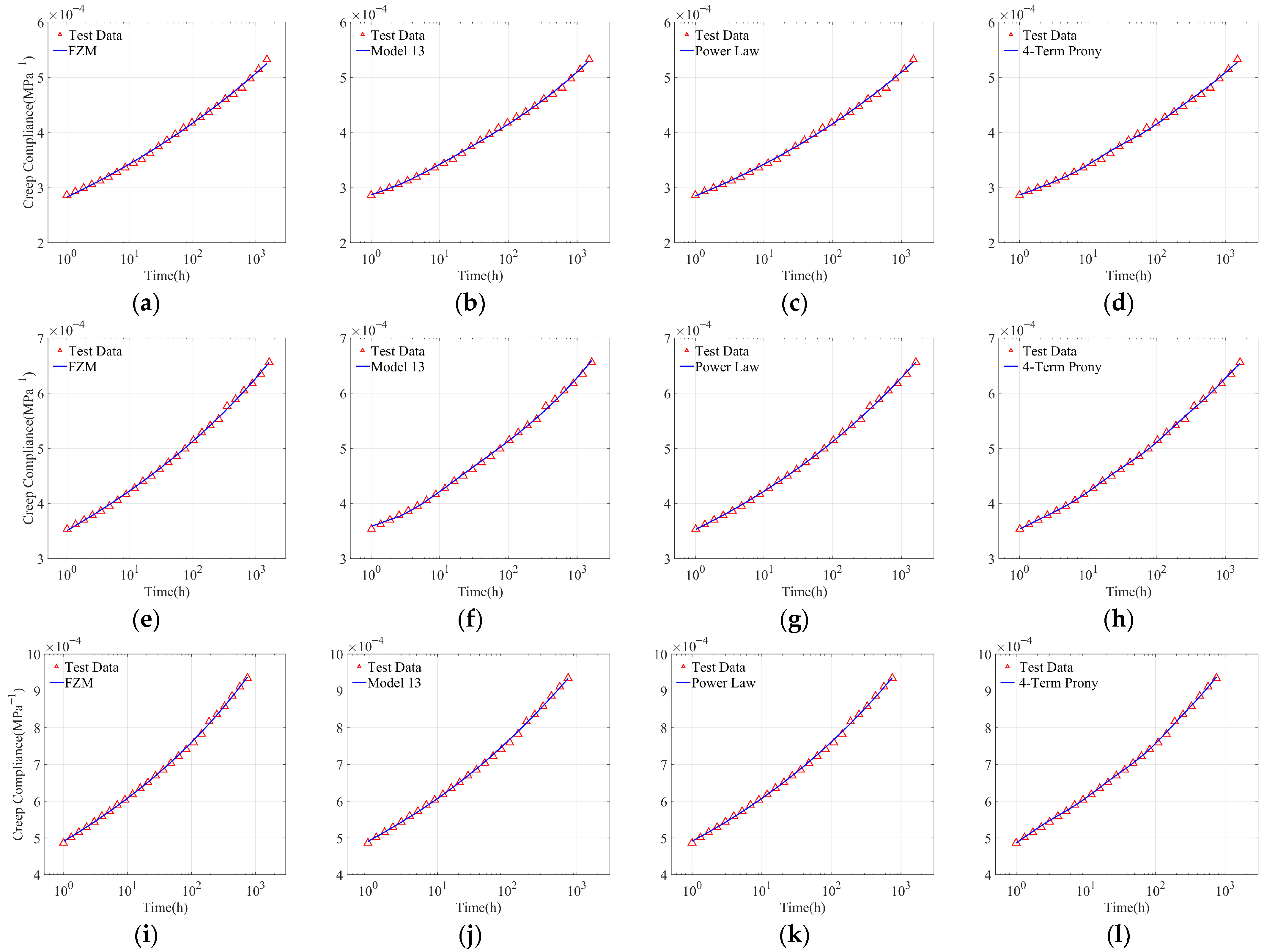
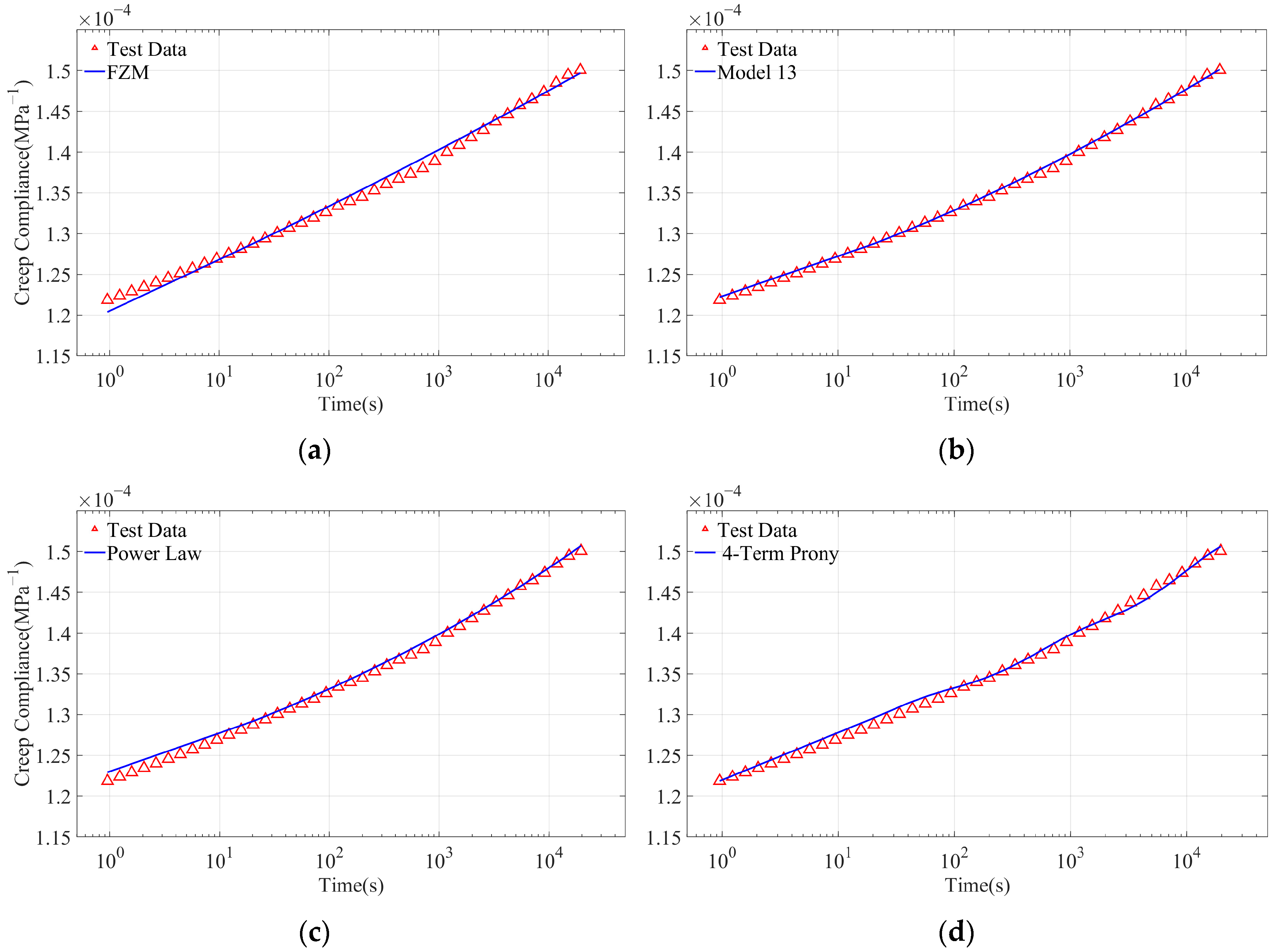
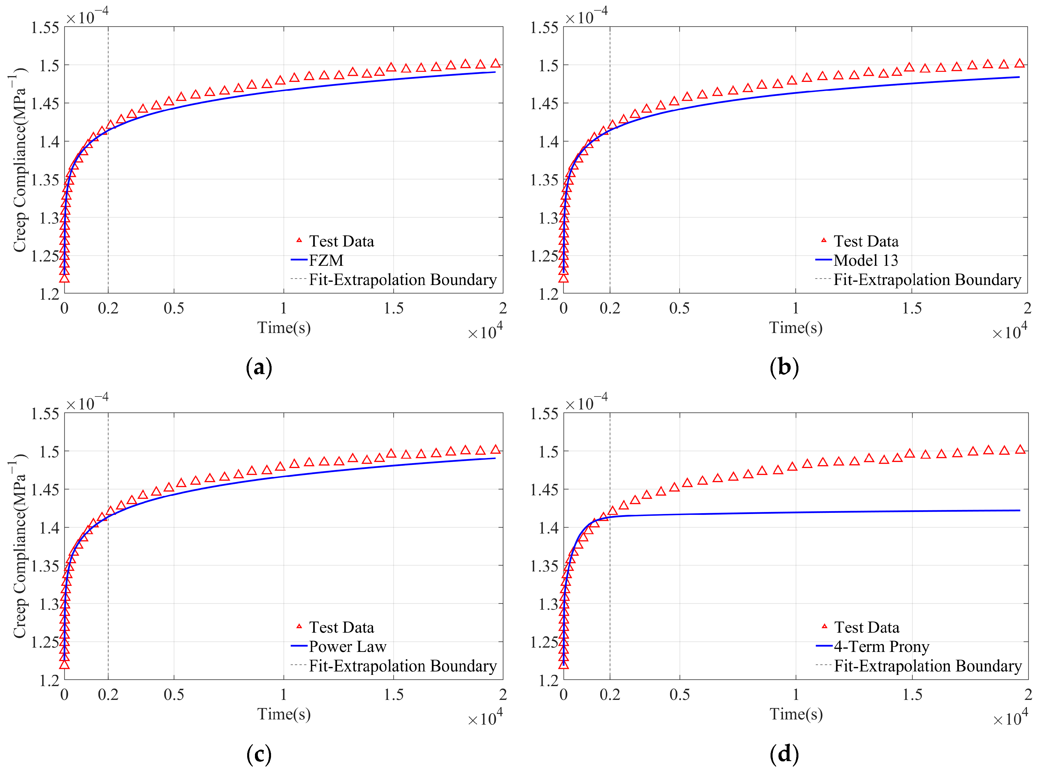
To provide an additional check beyond the published datasets, tensile creep data for a TATB-based PBX were obtained at 20 °C under a stress level of 5 MPa using an electronic universal testing machine. The creep strain was measured using an extensometer. The specimens were fabricated by hot isostatic pressing and machined into dog-bone-shaped specimens according to GJB 772A-1997 [41]. The specimens were first loaded to 5 MPa under displacement control at 0.5 mm/min, after which the stress was held constant for the creep test. The obtained creep data covered a time span of 0–20,000 s. The fitting performance of the fractional Zener model, Model 13, the power-law model, and the 3-term and 4-term Prony series models was further evaluated, as shown in Figure A1 and Table A14.
Figure A1. Fitting of creep data for PBX using fractional viscoelastic models and classical models (test data): (a) fractional Zener model; (b) Model 13; (c) power-law model; (d) 4-term Prony series.
Polymers 18 01430 g0a1
Table A14. Coefficients of determination and Akaike information criterion corresponding to the compared models for the in-house TATB-based PBX creep data.
ModelFZMModel 13Power Law3-Term Prony4-Term Prony
R 2 0.99060.99740.99780.97820.9968
A I C −1034.6818−1083.4135−1074.6890−1007.5034−1076.8689
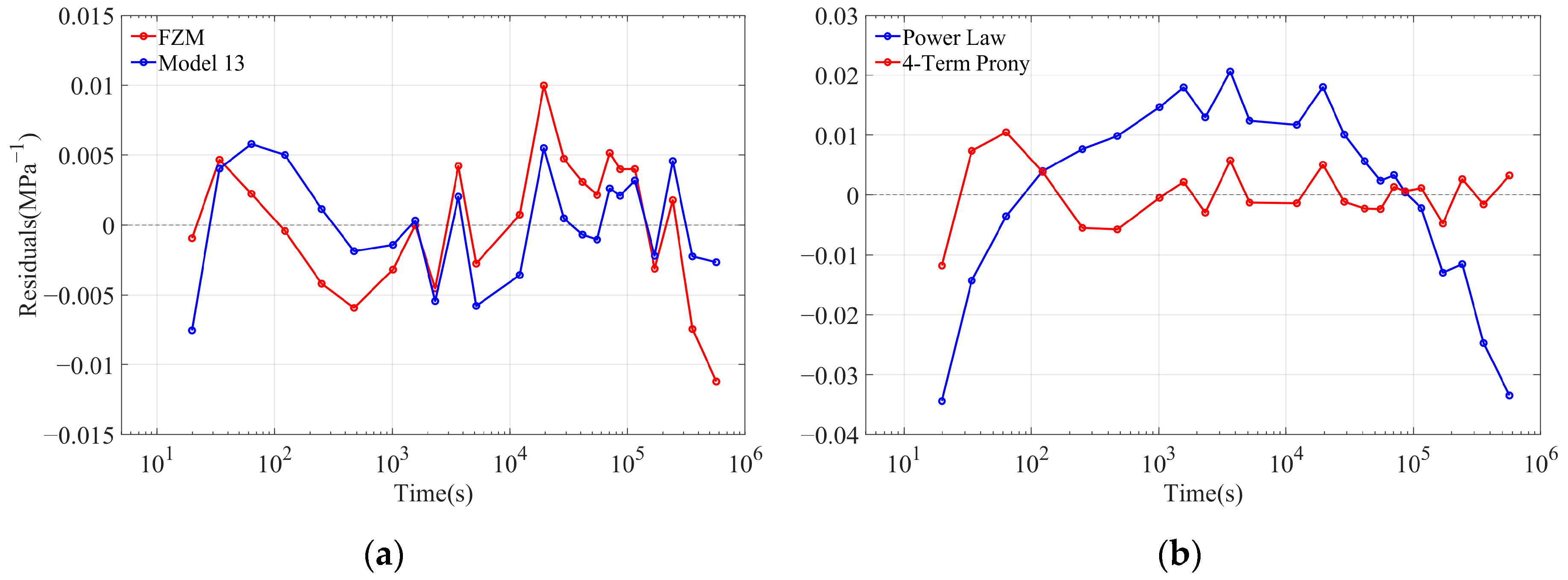
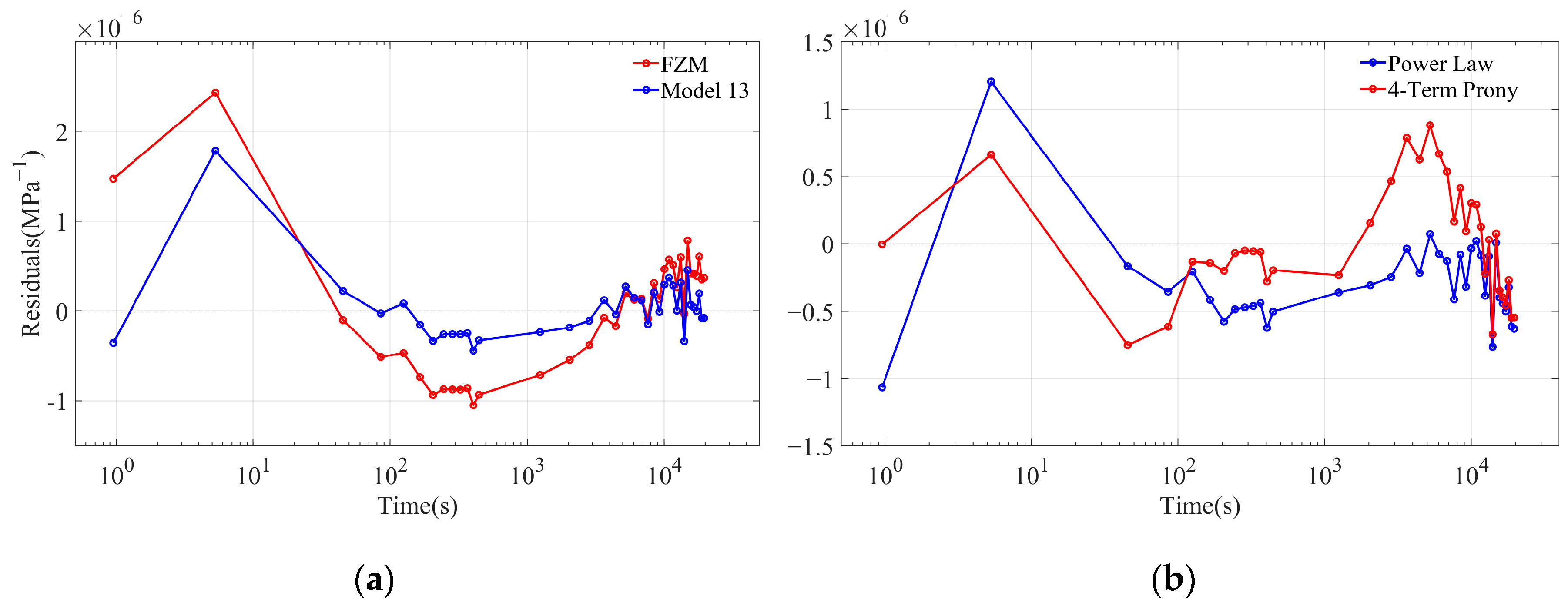
All models except the 3-term Prony series achieved satisfactory fitting performance for the experimentally obtained tensile creep data of the TATB-based PBX. The fractional Zener model, Model 13, the power-law model, and the 4-term Prony series all gave coefficients of determination higher than 0.99. Among them, the power-law model yielded the highest R 2 value ( R 2 = 0.9978 ), followed closely by Model 13 ( R 2 = 0.9974 ) and the 4-term Prony series ( R 2 = 0.9968 ). When model complexity was further considered using AIC, Model 13 exhibited the lowest AIC value ( A I C = 1083.4135 ), indicating the most favorable balance between fitting accuracy and parameter complexity for this dataset. The residual plots in Figure A2 further support this result. The residuals of the fractional Zener model and Model 13 were distributed relatively uniformly around zero over the investigated time range, without obvious systematic deviation, indicating that these models captured both early-stage and long-time creep responses of the TATB-based PBX.
These supplementary results based on independently measured TATB-based PBX creep data are consistent with the main trends obtained from the published datasets. In particular, Model 13 and the fractional Zener model provided accurate creep descriptions with a limited number of parameters, while maintaining favorable parameter efficiency and rheological interpretability. Therefore, the additional dataset supports the applicability of the selected fractional models to PBX creep analysis. Nevertheless, this supplementary assessment should be regarded as an additional consistency check rather than as complete independent validation over all loading conditions.
Figure A2. Residuals versus time of creep data for PBX using fractional viscoelastic models and classical models (test data): (a) fractional Zener model and Model 13; (b) power-law model and 4-term Prony series.
Polymers 18 01430 g0a2
As shown in Figure A3 and Table A15, when the first 10% time span of the experimentally obtained TATB-based PBX creep data was used for parameter identification, the fractional Zener model, Model 13, and the power-law model all exhibited satisfactory extrapolation performance, whereas the Prony series models showed much less stable extrapolation behavior.
Figure A3. Extrapolation results for the creep data for PBX using fractional viscoelastic models and classical models (test data): (a) fractional Zener model; (b) Model 13; (c) power-law model; (d) 4-term Prony series.
Polymers 18 01430 g0a3
Table A15. Extrapolation performance of the compared models for the in-house TATB-based PBX creep data.
ModelFZMModel 13Power Law3-Term Prony4-Term Prony
R 2 0.98490.97340.9848−0.79870.6046
r R M S E 0.76%1.03%0.76%8.76%4.10%
Overall, the selected low-order fractional viscoelastic models, especially the fractional Zener model and Model 13, showed acceptable extrapolation performance with a limited number of parameters. In particular, the fractional Zener model and Model 13 achieved low rRMSE values of 0.76% and 1.03%, respectively, indicating that both fractional models can provide reliable extrapolation for PBX creep data characterized by moderate steady-state creep rates.

Appendix D. Stability of Parameter Identification

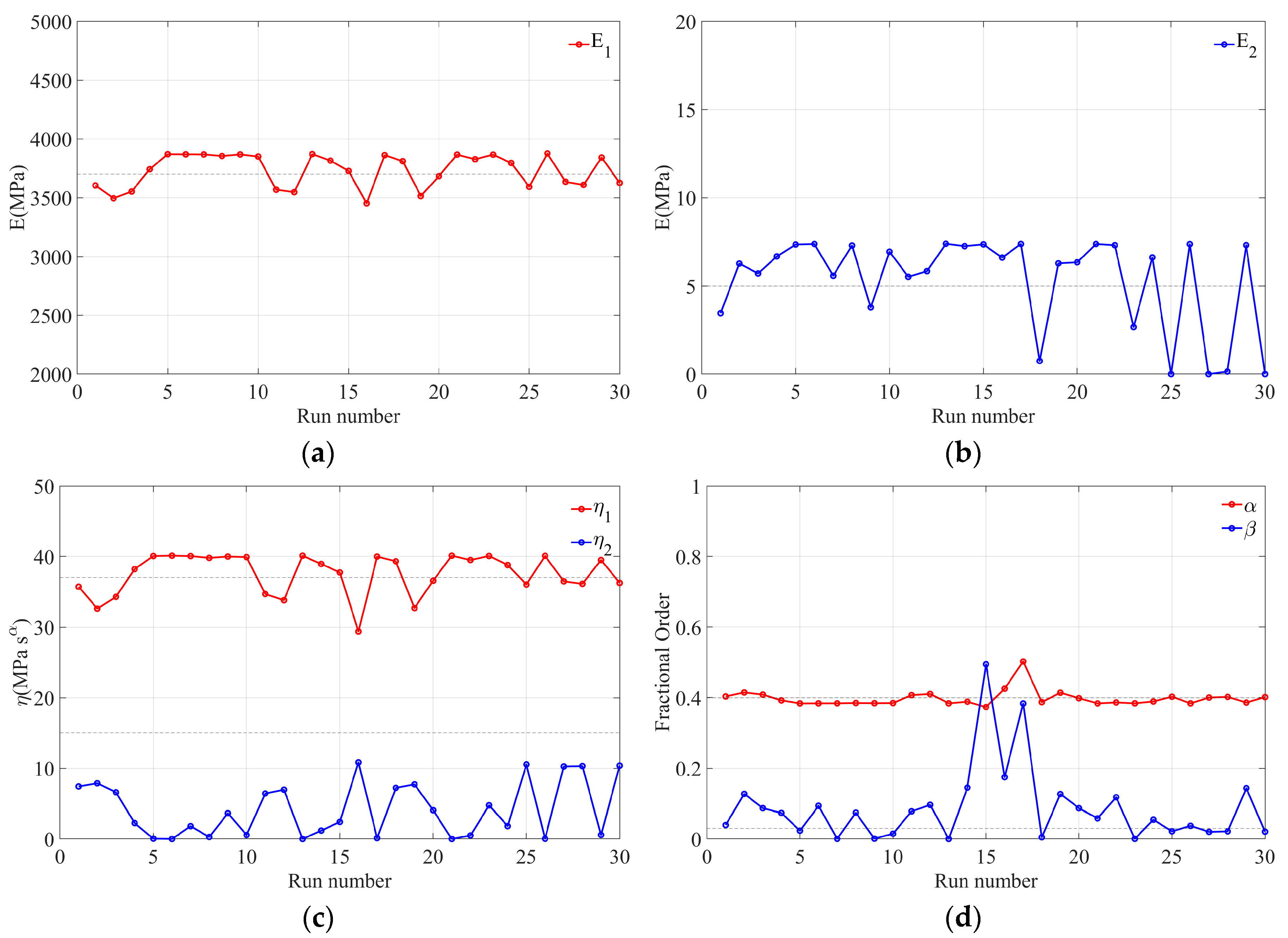
To further evaluate the stability of the parameter identification procedure, 30 independent optimization runs were performed for the same model and dataset using different random streams. The identified parameters from these runs were statistically analyzed, and their distributions are shown in Figure A4. Specifically, E 1 was mainly distributed within 3400–3900 MPa and E 2 within 0–8 MPa, while η 1 and η 2 were mainly distributed within 0–11 M P a · s α and 29–41 M P a · s β , respectively. The fractional order α fluctuated around 0.4, whereas β was distributed within 0–0.5. Although moderate variations were observed for some parameters, the overall distributions remained bound and showed no significant divergence among different runs. This indicates that the optimization process converged toward a stable parameter region rather than randomly scattered local solutions.
Figure A4. Distributions of the identified parameters obtained from 30 independent optimization runs for fitting Model 13 to the PVC/AP relaxation master curve (a) E 1 ; (b) E 2 ; (c) η 1 and η 2 ; (d) α and β .
Polymers 18 01430 g0a4
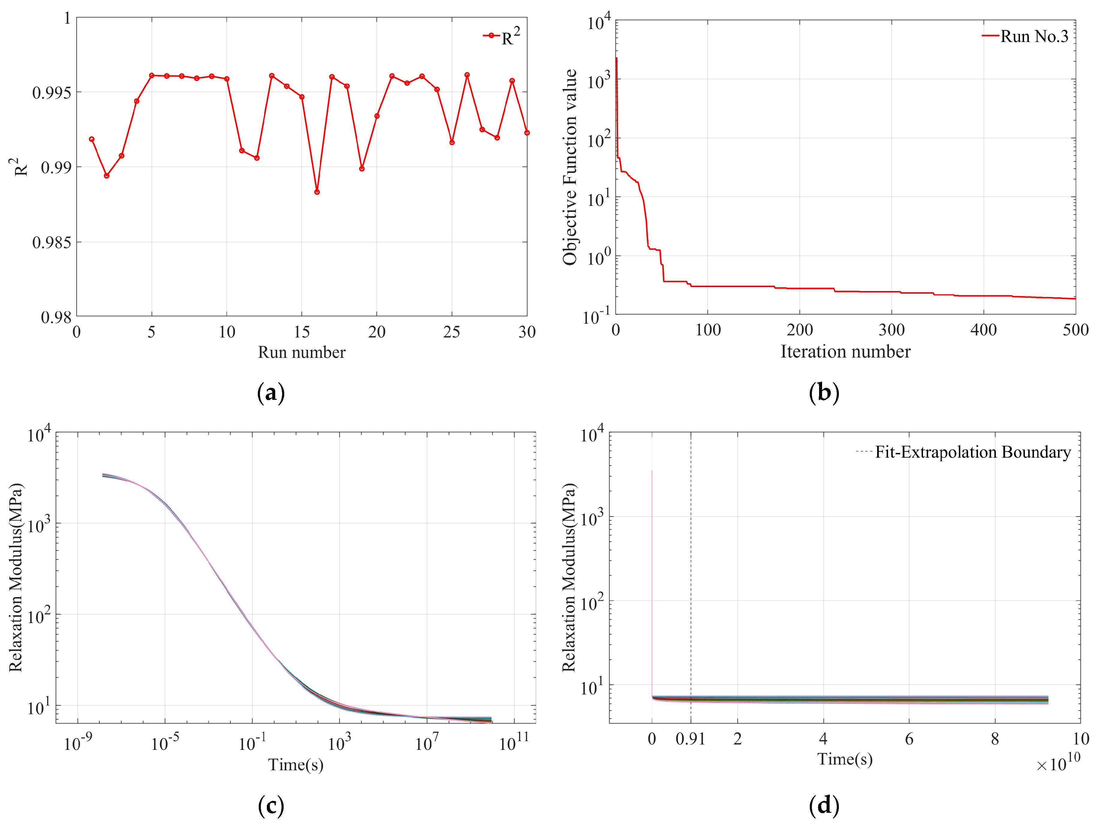
The consistently high R 2 values in Figure A5a further indicate that Model 13 maintained stable descriptive accuracy under different random initializations. The convergence history of the third independent run, shown in Figure A5b, exhibits a rapid decrease in the objective function during the early iterations, followed by a stable plateau. This indicates effective convergence of the optimization process.
The fitted curves obtained from the 30 independent runs almost overlapped with each other and closely followed the PVC/AP relaxation master curve, as shown in Figure A5c. Moreover, the corresponding extrapolated curves over the approximately one-order-of-magnitude longer time window also showed negligible differences, as shown in Figure A5d. These results suggest that moderate variations in individual parameters had limited influence on the macroscopic relaxation response and its early-stage data extrapolation behavior.
Figure A5. Response-level stability and convergence behavior obtained from 30 independent optimization runs for fitting Model 13 to the PVC/AP relaxation master curve: (a) R 2 values; (b) convergence history of the best objective value in the third independent run; (c) fitted curves obtained from the 30 independent runs; (d) extrapolated curves over the approximately one-order-of-magnitude longer time window.
Polymers 18 01430 g0a5
To examine possible parameter coupling, the correlation coefficients among the identified parameters ( E 1 ,   E 2 ,   η 1 ,   η 2 ,   α ,   β ) from the 30 independent runs were calculated, as shown in Matrix (A1). The correlation matrix indicates that some parameters were moderately or strongly correlated, suggesting that the identified parameter set may not be strictly unique. This behavior is common in multi-parameter fractional viscoelastic models, where different parameter combinations can produce similar macroscopic responses. Nevertheless, the fitted relaxation curves and the corresponding extrapolated curves remained nearly unchanged among the 30 independent runs. This indicates that, although parameter correlation exists, the response-level identification result is stable for the representative case considered.
C = [ 1 0.3260 0.9733 0.8450 0.3409 0.0900 0.3260 1 0.1890 0.7592 0.0085 0.1356 0.9733 0.1890 1 0.7814 0.3617 0.1356 0.8450 0.7592 0.7814 1 0.2425 0.1640 0.3409 0.0085 0.3617 0.2425 1 0.4217 0.0900 0.1356 0.1356 0.1640 0.4217 1 ] ,
Overall, the repeated identification results and parameter correlation analysis support the stability of the combined Talbot–Gray Wolf parameter identification procedure at the response level for the representative case considered. Although individual parameters may exhibit correlation and are not necessarily uniquely determined, the fitted and extrapolated curves remain nearly unchanged among independent runs. These results support response-level stability of the identification procedure for the representative case, although they also indicate that strict parameter uniqueness cannot be guaranteed.

References

  1. Arora, H.; Tarleton, E.; Li-Mayer, J.; Charalambides, M.N.; Lewis, D. Modelling the Damage and Deformation Process in a Plastic Bonded Explosive Microstructure under Tension Using the Finite Element Method. Comput. Mater. Sci. 2015, 110, 91–101. [Google Scholar] [CrossRef]
  2. Li, H.; Song, Q.; Wu, X.; Xu, J.; Chen, X. Research on the Statistical Damage Constitutive Model for Composite Solid Propellant. J. Phys. Conf. Ser. 2022, 2235, 012059. [Google Scholar] [CrossRef]
  3. Heider, N.; Steinbrenner, A.; Aurich, H. A Method for the Determination of the Viscoelastic Relaxation Modules of PBX by Confined SHPB Measurements. J. Dyn. Behav. Mater. 2017, 3, 133–150. [Google Scholar] [CrossRef]
  4. Cui, H.; Shen, Z.; Li, H. A New Constitutive Equation for Solid Propellant with the Effects of Aging and Viscoelastic Poisson’s Ratio. Meccanica 2018, 53, 2393–2410. [Google Scholar] [CrossRef]
  5. Deng, K.; Li, H.; Xu, J.; Cui, H.; Shen, Z. Long-Term and Short-Term Creep Characteristic Analysis for HTPB Propellant. Propellants Explos. Pyrotech. 2022, 47, e202200074. [Google Scholar] [CrossRef]
  6. Plassart, G.; Picart, D.; Gratton, M.; Frachon, A.; Caliez, M. Quasistatic Mechanical Behavior of HMX- and TATB-Based Plastic-Bonded Explosives. Mech. Mater. 2020, 150, 103561. [Google Scholar] [CrossRef]
  7. Lv, L.; Zhang, W.; Pan, X.; Li, G.; Zhang, C. PBX Micro Defect Characterization by Using Deep Learning and Image Processing of Micro CT Images. Energetic Mater. Front. 2025, 6, 177–188. [Google Scholar] [CrossRef]
  8. Jaishankar, A.; McKinley, G.H. Power-Law Rheology in the Bulk and at the Interface: Quasi-Properties and Fractional Constitutive Equations. Proc. R. Soc. A Math. Phys. Eng. Sci. 2013, 469, 20120284. [Google Scholar] [CrossRef]
  9. Bonfanti, A.; Kaplan, J.L.; Charras, G.; Kabla, A. Fractional Viscoelastic Models for Power-Law Materials. Soft Matter 2020, 16, 6002–6020. [Google Scholar] [CrossRef]
  10. Zhao, L.; Yuan, H.W.; Zhu, X.Y. Applicability Analysis of Time-temperature-stress Equivalent Principle in Tensile Creep of TATB-Based PBX. Chin. J. Energetic Mater. 2022, 30, 971–977. [Google Scholar]
  11. Feng, S.X.; Qiang, H.F.; Liu, Y.X.; Wang, X.R.; Geng, T.J.; Yang, Z.W. Research on Creep Constitutive and Numerical Simulation of Composite Solid Propellant. J. Phys. Conf. Ser. 2021, 1786, 012002. [Google Scholar] [CrossRef]
  12. Tschoegl, N.W. The Phenomenological Theory of Linear Viscoelastic Behavior; Springer: Berlin/Heidelberg, Germany, 1989; pp. 119–127. [Google Scholar]
  13. Lin, C.; Liu, J.; Huang, Z.; Gong, F.; Li, Y.; Pan, L.; Zhang, J.; Liu, S. Enhancement of Creep Properties of TATB-Based Polymer-Bonded Explosive Using Styrene Copolymer. Propellants Explos. Pyrotech. 2015, 40, 189–196. [Google Scholar] [CrossRef]
  14. Blair, G.W.S.; Veinoglou, B.C.; Caffyn, J.E. Limitations of the Newtonian Time Scale in Relation to Non-Equilibrium Rheological States and a Theory of Quasi-Properties. Proc. R. Soc. London. Ser. A Math. Phys. Sci. 1947, 189, 69–87. [Google Scholar] [CrossRef]
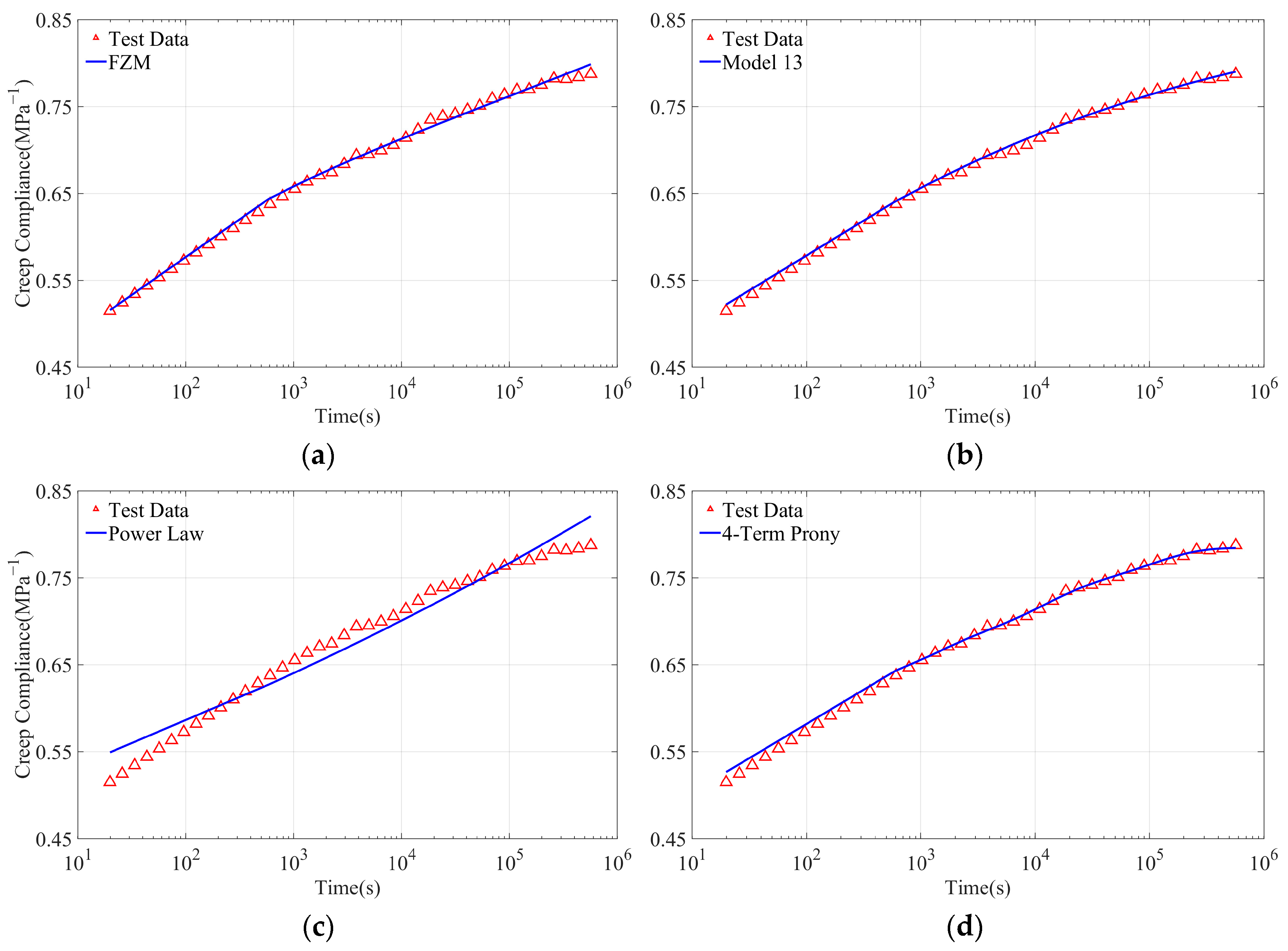
  15. Ferrás, L.L. Fractional Derivatives: The Ultimate Operator for Modelling Complex Viscoelastic Materials? Fract. Calc. Appl. Anal. 2025, 28, 2799–2848. [Google Scholar] [CrossRef]
  16. Koeller, R.C. Applications of Fractional Calculus to the Theory of Viscoelasticity. J. Appl. Mech. 1984, 51, 299–307. [Google Scholar] [CrossRef]
  17. Friedrich, C. Relaxation and Retardation Functions of the Maxwell Model with Fractional Derivatives. Rheol. Acta 1991, 30, 151–158. [Google Scholar] [CrossRef]
  18. Schiessel, H.; Metzler, R.; Blumen, A.; Nonnenmacher, T.F. Generalized Viscoelastic Models: Their Fractional Equations with Solutions. J. Phys. A Math. Gen. 1995, 28, 6567–6584. [Google Scholar] [CrossRef]
  19. Mainardi, F.; Spada, G. Creep, Relaxation and Viscosity Properties for Basic Fractional Models in Rheology. Eur. Phys. J. Spec. Top. 2011, 193, 133–160. [Google Scholar] [CrossRef]
  20. Atanacković, T.M.; Konjik, S.; Pilipović, S.; Zorica, D. Complex Order Fractional Derivatives in Viscoelasticity. Mech. Time-Depend. Mater. 2016, 20, 175–195. [Google Scholar] [CrossRef]
  21. Long, J.; Xiao, R.; Chen, W. Fractional Viscoelastic Models with Non-Singular Kernels. Mech. Mater. 2018, 127, 55–64. [Google Scholar] [CrossRef]
  22. Fang, C.; Shen, X.; He, K.; Yin, C.; Li, S.; Chen, X.; Sun, H. Application of Fractional Calculus Methods to Viscoelastic Behaviours of Solid Propellants. Philos. Trans. R. Soc. A Math. Phys. Eng. Sci. 2020, 378, 20190291. [Google Scholar] [CrossRef]
  23. Zhang, W.; Zhang, D.; Lei, Y.; Shen, Z. Research on the Low-Frequency Fatigue Behavior of NEPE Solid Composite Propellant Based on Fractional Derivative Constitutive Model. Int. J. Solids Struct. 2024, 300, 112931. [Google Scholar] [CrossRef]
  24. Caputo, M. Linear Models of Dissipation whose Q is almost Frequency Independent—II. Geophys. J. Int. 1967, 13, 529–539. [Google Scholar] [CrossRef]
  25. Li, C.; Qian, D.; Chen, Y. On Riemann-Liouville and Caputo Derivatives. Discret. Dyn. Nat. Soc. 2011, 2011, 562494. [Google Scholar] [CrossRef]
  26. Blair, G.S.; Coppen, F. The Subjective Conception of the Firmness of the Soft Materials. Am. J. Psychol. 1942, 55, 215–229. [Google Scholar] [CrossRef]
  27. Blair, G.S.; Coppen, F. The Estimation of Firmness in Soft Materials. Am. J. Psychol. 1943, 56, 234–246. [Google Scholar] [CrossRef]
  28. Liu, J.G.; Xu, M.Y. Higher-Order Fractional Constitutive Equations of Viscoelastic Materials Involving Three Different Parameters and Their Relaxation and Creep Functions. Mech. Time-Depend. Mater. 2006, 10, 263–279. [Google Scholar] [CrossRef]
  29. Yang, X.; Li, Q.; Shen, C. Viscosity Model Data Fitting for Polymer Melt Based on Golden Section Method. J. Mech. Eng. 2014, 50, 70–76. [Google Scholar] [CrossRef]
  30. Lewandowski, R.; Chorążyczewski, B. Identification of the Parameters of the Kelvin–Voigt and the Maxwell Fractional Models, Used to Modeling of Viscoelastic Dampers. Comput. Struct. 2010, 88, 1–17. [Google Scholar] [CrossRef]
  31. Ghazizadeh, H.R.; Azimi, A.; Maerefat, M. An Inverse Problem to Estimate Relaxation Parameter and Order of Fractionality in Fractional Single-Phase-Lag Heat Equation. Int. J. Heat Mass Transf. 2012, 55, 2095–2101. [Google Scholar] [CrossRef]
  32. Fan, W.; Jiang, X.; Qi, H. Parameter Estimation for the Generalized Fractional Element Network Zener Model Based on the Bayesian Method. Phys. A Stat. Mech. Appl. 2015, 427, 40–49. [Google Scholar] [CrossRef]
  33. Dabiri, D.; Saadat, M.; Mangal, D.; Jamali, S. Fractional Rheology-Informed Neural Networks for Data-Driven Identification of Viscoelastic Constitutive Models. Rheol. Acta 2023, 62, 557–568. [Google Scholar] [CrossRef]
  34. Talbot, A. The Accurate Numerical Inversion of Laplace Transforms. IMA J. Appl. Math. 1979, 23, 97–120. [Google Scholar] [CrossRef]
  35. Makhadmeh, S.N.; Al-Betar, M.A.; Doush, I.A.; Awadallah, M.A.; Kassaymeh, S.; Mirjalili, S.; Zitar, R.A. Recent Advances in Grey Wolf Optimizer, Its Versions and Applications: Review. IEEE Access 2024, 12, 22991–23028. [Google Scholar] [CrossRef]
  36. Mirjalili, S.; Mirjalili, S.M.; Lewis, A. Grey Wolf Optimizer. Adv. Eng. Softw. 2014, 69, 46–61. [Google Scholar] [CrossRef]
  37. Zhao, B.; Xin, Z. Spectrum of Viscoelasticity of a Composite Solid Propellant (PVC/AP). J. Beijing Inst. Technol. 1986, 1, 106–118. [Google Scholar]
  38. Xiao, Y.C.; Sun, Y.; Wang, Z.J. Investigating the Static and Dynamic Tensile Mechanical Behaviour of Polymer-bonded Explosives. Strain 2018, 54, e12262. [Google Scholar] [CrossRef]
  39. Trujillo, D.J.; Thompson, D.G. Memo WX7-14-1359, Subject: PBX 9502 Creep Data, Compression and Tension; Los Alamos National Laboratory: Los Alamos, NM, USA, 2014; LA-UR-14-20710. [Google Scholar]
  40. Zhang, Y.; Deng, K.; Shen, Z. Long-Term Creep Prediction of NEPE Propellant Based on SSM Method. Propellants Explos. Pyrotech. 2024, 49, e202400159. [Google Scholar] [CrossRef]
  41. GJB 772A-1997; Explosives Test Methods. General Armament Department: Beijing, China, 1997.
Figure 1. Schematic of the fractional rheological element (spring-pot), where E denotes the elastic modulus, η is the “firmness” and η 1 is the viscosity parameter. For the spring-pot relation σ ( t ) = η D t α ε ( t ) , the parameter η has the unit of M P a · s α when strain is dimensionless. More generally, a spring-pot coefficient of order β has the unit of M P a · s β . These parameters should be interpreted as effective rheological coefficients rather than conventional viscosity constants.
Polymers 18 01430 g001
Figure 2. Mechanical analogy and constitutive equations of two elements in series: (a) spring; (b) dashpot; (c) fractional rheological element.
Polymers 18 01430 g002
Figure 3. Mechanical analogy of Model 13 in Appendix A.
Polymers 18 01430 g003
Figure 4. Fitting of relaxation data for solid propellant (PVC/AP) using fractional viscoelastic models and classical models: (a) fractional Zener model; (b) Model 13; (c) the fractional model proposed by Fang et al. [22]; (d) power-law model; (e) 9-term Prony series.
Polymers 18 01430 g004
Figure 5. Residuals versus time of relaxation data for solid propellant (PVC/AP) using fractional viscoelastic models and classical models: (a) fractional Zener model, Model 13, and the fractional model proposed by Fang et al. [22]; (b) power-law model and 9-term Prony series.
Polymers 18 01430 g005
Figure 6. Fitting of relaxation data for PBX using fractional viscoelastic models and classical models: (a) fractional Zener model; (b) Model 13; (c) power-law model; (d) 6-term Prony series.
Polymers 18 01430 g006
Figure 7. Residuals versus time of relaxation data for PBX using fractional viscoelastic models and classical models: (a) fractional Zener model and Model 13; (b) power-law model and 6-term Prony series.
Polymers 18 01430 g007
Figure 8. Fitting results for the compressive creep data of PBX under different load and temperature conditions: (a) fractional Zener model at −3 MPa and 40 °C; (b) Model 13 at −3 MPa and 40 °C; (c) power-law model at −3 MPa and 40 °C; (d) 4-term Prony series at −3 MPa and 40 °C; (e) fractional Zener model at −4 MPa and 40 °C; (f) Model 13 at −4 MPa and 40 °C; (g) power-law model at −4 MPa and 40 °C; (h) 4-term Prony series at −4 MPa and 40 °C; (i) fractional Zener model at −5 MPa and 50 °C; (j) Model 13 at −5 MPa and 50 °C; (k) power-law model at −5 MPa and 50 °C; (l) 4-term Prony series at −5 MPa and 50 °C.
Polymers 18 01430 g008
Figure 9. Residuals versus time for the fitted compressive creep data of PBX under different load and temperature conditions: (a) fractional Zener model and Model 13 at −3 MPa and 40 °C; (b) power-law model and 4-term Prony series at −3 MPa and 40 °C; (c) fractional Zener model and Model 13 at −4 MPa and 40 °C; (d) power-law model and 4-term Prony series at −4 MPa and 40 °C; (e) fractional Zener model and Model 13 at −5 MPa and 50 °C; (f) power-law model and 4-term Prony series at −5 MPa and 50 °C.
Polymers 18 01430 g009
Figure 10. Fitting of creep data for NEPE propellant using fractional viscoelastic models and classical models: (a) fractional Zener model; (b) Model 13; (c) power-law model; (d) 4-term Prony series.
Polymers 18 01430 g010
Figure 11. Residuals versus time of creep data for NEPE propellant using fractional viscoelastic models and classical models: (a) fractional Zener model and Model 13; (b) power-law model and 4-term Prony series.
Polymers 18 01430 g011
Figure 12. Extrapolation results of relaxation data for solid propellant (PVC/AP) using fractional viscoelastic models and classical models: (a) fractional Zener model; (b) Model 13; (c) power-law model; (d) 9-term Prony series.
Polymers 18 01430 g012
Figure 13. Extrapolation results of relaxation data for PBX using fractional viscoelastic models and classical models: (a) fractional Zener model; (b) Model 13; (c) power-law model; (d) 6-term Prony series.
Polymers 18 01430 g013
Figure 14. Extrapolation results for the compressive creep data of PBX under different load and temperature conditions using fractional viscoelastic and classical models: (a) fractional Zener model at −3 MPa and 40 °C; (b) Model 13 at −3 MPa and 40 °C; (c) power-law model at −3 MPa and 40 °C; (d) 4-term Prony series at −3 MPa and 40 °C; (e) fractional Zener model at −4 MPa and 40 °C; (f) Model 13 at −4 MPa and 40 °C; (g) power-law model at −4 MPa and 40 °C; (h) 4-term Prony series at −4 MPa and 40 °C; (i) fractional Zener model at −5 MPa and 50 °C; (j) Model 13 at −5 MPa and 50 °C; (k) power-law model at −5 MPa and 50 °C; (l) 4-term Prony series at −5 MPa and 50 °C.
Polymers 18 01430 g014
Figure 15. Extrapolation results for the creep data for NEPE propellant using fractional viscoelastic models and classical models: (a) fractional Zener model; (b) Model 13; (c) power-law model; (d) 4-term Prony series.
Polymers 18 01430 g015
Table 1. Numerical settings for parameter identification.
ItemSetting
Numerical inverse Laplace methodTalbot method
Number of Talbot truncation terms64
OptimizerGray Wolf Optimizer
Population size40
Maximum iterations500
Random seed2025
Lower bounds of all parameters0
Fractional-order bounds[0, 1]
Termination criterionMaximum iteration number
Objective functionSum of squared relative errors
Table 2. Coefficients of determination and Akaike information criterion corresponding to the compared models for the solid propellant (PVC/AP) relaxation data.
ModelFZMModel 13Fang et al.’s Fractional Model [22]Power Law9-Term Prony
R 2 0.99880.99190.99600.77720.9976
A I C 340.7258429.1384398.4827575.3599399.7494
Table 3. Coefficients of determination and Akaike information criterion corresponding to the compared models for the PBX relaxation data.
ModelFZMModel 13Power Law4-Term Prony5-Term Prony6-Term Prony
R 2 0.99970.99990.99900.98130.99080.9977
A I C −58.6022−100.9052−8.3533140.1445110.968848.6924
Table 4. Coefficients of determination and Akaike information criterion corresponding to the compared models for the PBX compression creep data.
ModelFZMModel 13Power Law3-Term Prony4-Term Prony
R 2 ( 3   MPa ) 0.99820.99870.99840.99780.9983
A I C ( 3   MPa ) −444.0164−449.7906−452.8295−444.7925−446.9092
R 2 ( 4   MPa ) 0.99940.99910.99950.99880.9995
A I C ( 4   MPa ) −636.3960−625.0108−644.0084−621.7003−639.5528
R 2 ( 5   MPa ) 0.99940.99920.99920.99710.9996
A I C ( 5   MPa ) −390.1263−385.3738−392.8688−369.2515−400.2626
Table 5. Coefficients of determination and Akaike information criterion corresponding to the compared models for the NEPE propellant creep data.
ModelFZMModel 13Power Law3-Term Prony4-Term Prony
R 2 0.99640.99790.96260.98410.9965
A I C −233.8027−245.9398−185.7660−203.4257−236.2729
Table 6. Extrapolation performance of the compared models for the solid propellant (PVC/AP) relaxation data.
ModelFZMModel 13Power Law9-Term Prony
R 2 0.99220.99150.77760.9952
r R M S E 5.78%3.45%1.63%1.88%
Table 7. Extrapolation performance of the compared models for the PBX relaxation data.
ModelFZMModel 13Power Law4-Term Prony5-Term Prony6-Term Prony
R 2 0.99930.99980.9993−2.05370.98520.9969
r R M S E 8.43%2.37%8.45%100.11%33.37%13.21%
Table 8. Extrapolation performance of the compared models for the PBX compression creep data.
ModelFZMModel 13Power Law3-Term Prony4-Term Prony
R 2 ( 3   MPa ) 0.99790.93480.9587−0.57300.6832
r R M S E ( 3   MPa ) 0.95%6.73%5.34%33.13%14.85%
R 2 ( 4   MPa ) 0.99690.90990.9894−0.4400−1.0808
r R M S E ( 4   MPa ) 1.27%7.16%2.45%28.65%34.44%
R 2 ( 5   MPa ) 0.99430.87670.99370.68370.9822
r R M S E ( 5   MPa ) 1.74%8.19%1.84%13.08%3.11%
Table 9. Extrapolation performance of the compared models for the NEPE propellant creep data.
ModelFZMModel 13Power Law3-Term Prony4-Term Prony
R 2 0.95630.99790.34880.86900.9965
r R M S E 3.65%0.56%13.45%4.19%0.33%
Disclaimer/Publisher’s Note: The statements, opinions and data contained in all publications are solely those of the individual author(s) and contributor(s) and not of MDPI and/or the editor(s). MDPI and/or the editor(s) disclaim responsibility for any injury to people or property resulting from any ideas, methods, instructions or products referred to in the content.